Statistically-Based Comparison of the Removal Efficiencies and Resilience Capacities between Conventional and Natural Wastewater Treatment Systems: A Peak Load Scenario

Abstract

Emerging global threats, such as climate change, urbanization and water depletion, are driving forces for finding a feasible substitute for low cost-effective conventional activated sludge (AS) technology. On the other hand, given their low cost and easy operation, nature-based systems such as constructed wetlands (CWs) and waste stabilization ponds (WSPs) appear to be viable options. To examine these systems, a 210-day experiment with 31 days of peak load scenario was performed. Particularly, we conducted a deliberate strategy of experimentation, which includes applying a preliminary study, preliminary models, hypothetical tests and power analysis to compare their removal efficiencies and resilience capacities. In contrast to comparable high removal efficiencies of organic matter—around 90%—both natural systems showed moderate nutrient removal efficiencies, which inferred the necessity for further treatment to ensure their compliance with environmental standards. During the peak period, the pond treatment systems appeared to be the most robust as they indicated a higher strength to withstanding the organic matter and nitrogen shock load and were able to recover within a short period. However, high demand of land—2.5 times larger than that of AS—is a major concern of the applicability of WSPs despite their lower operation and maintenance (O&M) costs. It is also worth noting that initial efforts on systematic experimentation appeared to have an essential impact on ensuring statistically and practically meaningful results in this comparison study.

1. Introduction

Conventional activated sludge (AS) systems are widely applied to sewage treatment even though this approach has recently been criticized as a low cost-effective technology with high energy demand and limited recovery potential [1]. Because of that, together with a fast growing population resulting in a substantial increase in both water demand and water scarcity, viable alternatives are of key importance. A wide range of advanced mechanical treatment processes have been proposed, including membrane bioreactors, sand filtration and aerobic granulation. Despite their high performance, the applicability of these advanced technologies is still being questioned, especially in developing countries where around 90% of sewage is discharged untreated due to the barrier of affordability [2]. From that perspective, waste stabilization ponds (WSPs) and constructed wetlands (CWs), can be appropriate alternatives thanks to low cost and minimal operation and maintenance (O&M) requirements.

To assess the practicability and advisability of the application of the natural systems, a relevant experimental evaluation between AS and these natural systems is needed, as most of the comparisons have only been conducted in theory [3,4]. So far, theoretical comparisons have relied upon system-specific data collection from different sources, followed by a comparison of specific summarizing criteria: environmental performance, economic performance and societal sustainability. However, due to unreliable comparisons because of highly subjective criteria and the absence of specific scenarios to be investigated, conclusions have remained rather general such as ‘there is no ideal system applicable to all conditions’ (von Sperling [3], p. 61) or ‘difficulty in identifying a best overall option’ (Muga and Mihelcic [4], p. 445). More importantly, a key criterion of these systems was missing—their resilience to disruptions, which indicates the ability to adapt, endure and recover from changing conditions [5,6].

Since wastewater treatment plants (WWTPs) are normally long-lasting with an expected lifespan of 60 to 70 years, the pre-selection assessment between different systems should account for possible future challenges to minimize additional expenses from reconstructions and adjustments [7,8]. Recently, the New Jersey Department of Environmental Protection had to plan 1.7 billion dollars for rebuilding a sewage treatment system to become more resilient after Hurricane Sandy in 2012 [9]. Therefore, the goal of this work was to investigate and compare the removal efficiency and resilience capacity of three treatment systems: AS, CW and WSP. To this end, three lab-scale replicates of each system were run for 210 days during which we tested their resilience capacity over 31 days of peak scenario to high-strength wastewater. Conclusions about the performance were drawn as the results of four statistical tests. Ultimately, a specific evaluation of the applicability of the three systems was formed.

2. Materials and Methods

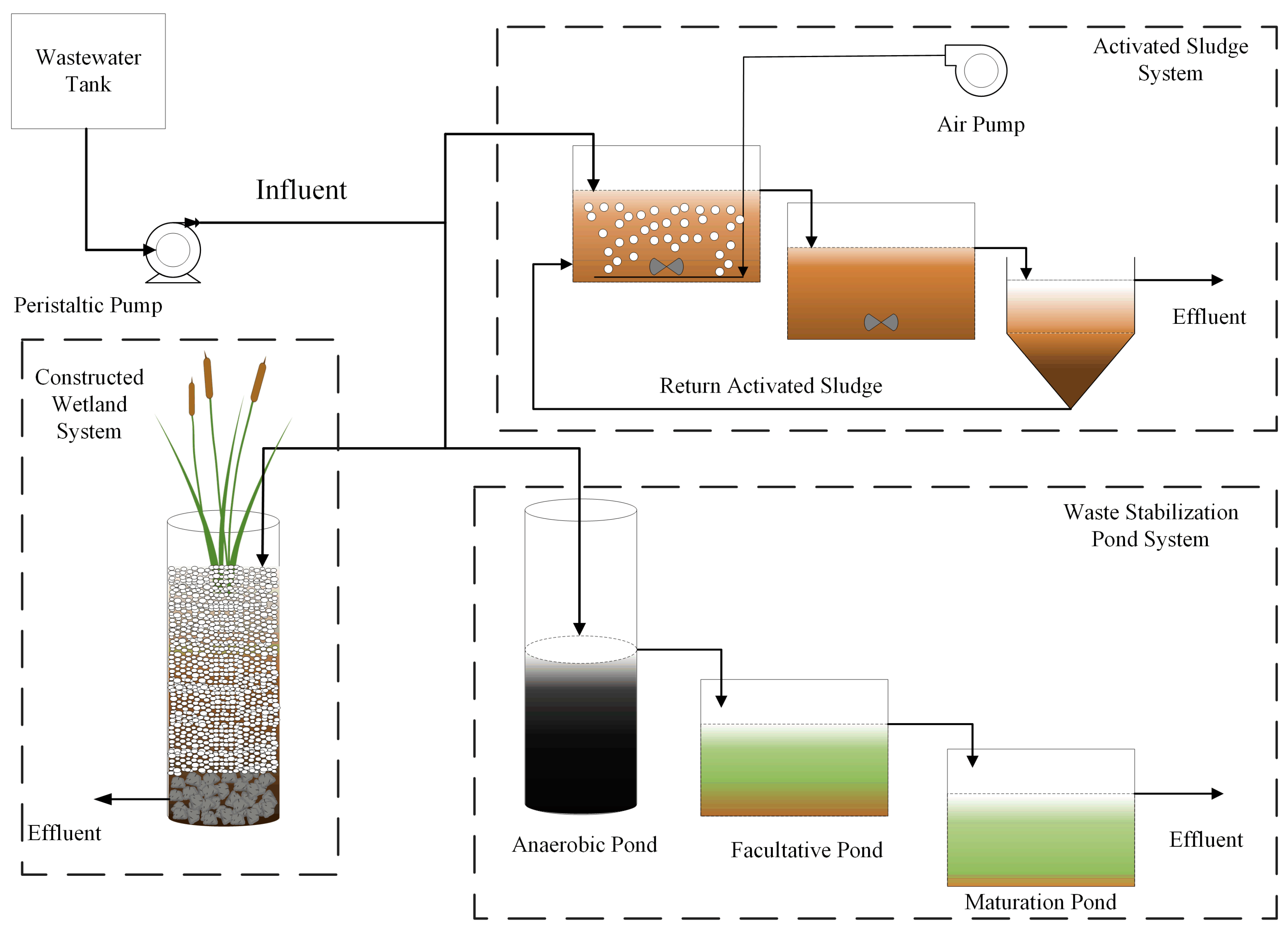
2.1. Experimental Setup

Lab-scale installations of the three systems were set up in triplicates in a temperature-controlled room with an air temperature of 21 (±2) °C (Figure 1). Standard fluorescent lamps provided 16 h of illumination per day-night cycle. Artificial wastewater was prepared every 1.5 days and fed continuously to the systems with an average flow of around three L·d⁻¹ for 210 days. The recipe for the artificial wastewater was based on the OECD [10] guideline resulting in BOD₅ of 150 mg O₂·L⁻¹, COD of 275 mg O₂·L⁻¹, total nitrogen (TN) of 40 mg N·L⁻¹ and total phosphorus (TP) of 7 mg P·L⁻¹. The reasons for using synthetic wastewater are: (1) its stability and controllable composition can expedite the long time period of the commissioning phase of the two natural systems; (2) low TSS concentrations before entering the three systems to avoid the clogging of pipes and vertical flow constructed wetland (VF CW) systems; (3) higher potential of replicability of the studies. For each treatment approach, a specific configuration was selected, that is, the Wuhrmann process for AS systems, conventional WSPs including three compartments in series, an anaerobic (AP), a facultative (FP) and a maturation (MP) pond and vertical flow constructed wetlands (VF CW) (Figure 1). These configurations were chosen based on their basic, conventional and common settings for removing organic matters and nutrients of the three systems. The comparisons of more advanced or combination configurations of the three systems merit different studies, hence, they are not considered in this study.

2.1.1. Activated Sludge Systems

The configuration of the AS system was installed following the Wuhrmann process in which the denitrification reactor was placed after the combined carbon oxidation/nitrification stage [11]. In particular, the AS system comprised two tanks of three litres each, with a dimension of 24.5 cm × 14.5 cm × 8.5 cm (L:W:H), which were gravitationally connected with each other to allow the free flow of wastewater. The system was inoculated with activated sludge from the domestic wastewater treatment plant of Ossemeersen, Gent (Aquafin) and the continuous suspension of sludge was ascertained via magnetic stirrers at the bottom of each tank. The first tank was aerated by air pumps to maintain dissolved oxygen (DO) concentration of 2–6 mg O₂·L⁻¹. Compared to recommended values 1.5–2 mg O₂·L⁻¹ by Metcalf, et al. [12], this relatively high DO concentration was provided to facilitate the nitrification rates in the aerated tank at high organic matter loads. The sludge in the settling compartment was recycled twice per day to the aerobic tank to maintain proper process-control values, that is, active biomass concentration of 3 g MLVSS·L⁻¹, food to microorganism ratio (F/M) of 0.20–0.25 g COD·g⁻¹ VSS·d⁻¹ and sludge volumetric index (SVI) from 60–100 mL·g⁻¹ in the two tanks [12]. These process-control measures were monitored on a daily basis to ensure the proper operation of the AS systems.

2.1.2. Constructed Wetlands

The lab-scale installation of vertical flow constructed wetland (VF CW) was installed in a PVC tube with a height of 1 m and a base diameter of 0.2 m. The medium of CW comprised two layers of substrates, 10 cm of coarse rock layer at the bottom and 70 cm of gravel layer with porosity of 30% piled on top. Systems were inoculated with one litre of AS from the WWTP of Ossemeersen, Gent (Aquafin) and had a final volume of about 7.5 L, resulting in a hydraulic retention time (HRT) of 2.2 days. Afterwards, two shoots of Typha latifolia from Geert Verhoeyen, Oeverplanten Company were planted in each replica. The wastewater was loaded on top of the substrate and the effluent was withdrawn from a plastic valve at the bottom. These settings were chosen following the studies of Sun and Austin [13] and Tang, et al. [14].

2.1.3. Waste Stabilization Ponds

The WSPs consisted of three compartments in series, an anaerobic (AP), a facultative (FP) and a maturation (MP) pond. More specifically, APs were set up in a cylindrical container with the same size as CW tubes yet their effluent valve was located in the middle of the tube, leading to 2.5 days of HRT. FPs and MPs were installed in plastic aquaria with dimensions 37 cm × 20 cm × 20 cm (L:W:H), resulting in a volume of 15 litres and a HRT of almost five days. The dimensions of these ponds were calculated based on the standard guideline of pond design [15,16,17,18]. More specifically, the volumetric loading rate of the APs during the standard influent was maintained around 400 g BOD₅·m⁻³·d⁻¹ while the surface loading rate of FPs was around 200 kg BOD₅·ha⁻¹·d⁻¹. Prior to the experiments, each AP was inoculated with five litres of anaerobic sludge from WWTP Aquafin Ossemeersen and both FP and MP were implanted with a consortium of microalgae.

2.2. Preliminary Studies

Main objectives of the start-up period are to: (1) get acquainted with the systems; (2) ensure the stability of the systems; (3) supply data required for calculating the kinetic rate of the predictive models; (4) provide information about the variability of samples and the related biologically relevant difference required for power analysis tests (see further). To do so, the start-up period was maintained for 179 days, with samples being collected and analysed two times per week. In particular, BOD₅ (mg O₂·L⁻¹) was analysed according to ISO 5815-1:2003 while COD (mg O₂·L⁻¹), TN (mg N·L⁻¹) and TP (mg P·L⁻¹) were determined via Merck Spectroquant analytical kits [19]. In addition, pH (-), temperature (T, °C), dissolved oxygen (DO, mg O₂·L⁻¹), electrical conductivity (EC, µS·cm⁻¹) and sludge volume index (SVI, mL·g⁻¹) were monitored on a daily basis.

2.3. Peak Load Scenario

After the stabilization period, the peak load scenario was implemented in three phases. Standard artificial wastewater was fed to the systems for eight days of the first phase. Subsequently, the influent pollutant concentrations were tripled, resulting in a high strength untreated domestic wastewater according to Metcalf, Eddy, Burton, Stensel and Tchobanoglous [12] and then kept for five days of the second phase. The recovery of the systems was followed for the next 18 days with the initial wastewater in the third phase. Before running this scenario, we expected that there would be differences in the response of the three systems due to the differences in their HRT and removal efficiencies as were determined in the preliminary period. Hence, we developed a deliberate strategy of experimentation including four following steps in order to design a better cost-effective sampling campaign and to avoid wastefully excessive sample collection.

2.3.1. Preliminary Models

The development of preliminary models allows improving the value of an experiment by decreasing the risk of failure and related costs, hence guarantees valuable results. The application of preliminary models simulates the possible responses of the three systems to the shock loads, allowing the fine-tuning of research questions and statistical hypotheses as well as supporting a better organization of the sampling campaign. More specifically, the kinetic removal rates of the three systems were calculated from the data of the start-up period, which, in turn, were applied in plug flow models to predict the effluent concentrations of the three systems during the disturbance. The first-order kinetic model was chosen as it was recommended as a good consensus between required efforts and confidence level in model outcomes by Rousseau, et al. [20] and Ho, Van Echelpoel and Goethals [16]. These simulations were performed for each parameter in a plug-flow advective-diffusive reactor compartment, with the AQUASIM software [21]. From the outcomes of these simulations, the predicted effluent concentrations of the systems were demonstrated as bell-shaped curves with three phases relevant to those in the influent (see Figures S1–S4).

2.3.2. Hypothesis Testing

A statistical hypothesis testing is used to achieve a judgement on a population where samples are taken, as a formalism of induction (from specific to general). The first step in statistical testing is to state a statistical null hypothesis (H₀), which, in our experiment, was a hypothesis of no difference between different treatment technologies. As such, four relevant null hypotheses were formed, relevant to the comparison of removal efficiency and resilience capacities of the three systems (see

Table 1. Four null hypotheses with the relevant objectives of this study for each of the following variables: BOD₅, COD, TN and TP.

Null Hypotheses	Performance Comparison
H01: The mean effluent concentrations of the three systems are equal during the first phase.	Removal capacity
H02: The mean effluent concentrations of the three systems are equal during the disturbance.	Resilience capacity
H03: The mean effluent concentrations of the three systems are equal during the recovering phase.	Removal capacity
H04: The mean effluent concentrations before and after the disturbance of each system are the same.	Recoverability

). These hypotheses were applied in all four variables, that is, BOD₅, COD, TN and TP.

In the second step of hypothesis testing, adequate statistical tests must be chosen. Standard tests, such as t-test statistics or ANOVA F-test statistics, were inadequate due to the spatial autocorrelation of the samples within a system [22]. Consequently, we employed likelihood ratio tests (LRTs) in context of linear mixed effect models (LMMs). More specifically, in case of the first three hypotheses, the spatial autocorrelation was considered in the random effect in the LMMs. Regarding the fix effect, as these concentrations varied with time and their removal efficiencies were different from one system to another, two explanatory variables were time and system. After constructing these models, we applied LRTs to compare likelihood function values between the mixed model and a reference model which was a multivariate linear regression model with the same fixed structure but without the random effect [23]. From that, we can determine the necessity to include this random effect, meaning that there was a difference among the three systems in terms of the effluent quality. Worth noting is that, in the last hypothesis, the mean effluent concentrations were compared before and after the disturbance in each system, hence, two phases were considered as the random effect which accounted for temporal autocorrelation. These statistical tests were executed in R [24] using the lme function in the nlme package [25].

2.3.3. Sample Size Determination

To avoid under- and over powering study, another crucial aspect of this experimental design is the determination of adequate sample size required to have sufficient statistical power (0.8) for identifying biological relevant differences between the three systems [26]. More importantly, since these differences had to be determined in each phase as stated in the hypotheses, the required sample size was calculated for each phase. To do so, we combined Monte Carlo methods with 1000 simulations in this power analysis since many advantages of this combination—such as higher accuracy and flexibility and ease of extension beyond hypothesis testing—were proved by Bolker [27]. Furthermore, since sample size determination for regression models in the standard procedure of power analysis was not appropriate in this case due to the spatial autocorrelation, mixed models were used [26]. In short, we conducted a simulation-based power analysis with different sample sizes in each phase to define their required values to obtain the statistical power of 0.8. These possible numbers of sample are 3–4 samples during the beginning period, 4–8 samples during the reaction period and 4–5 samples during the last period, making 11–17 samples in total. In these simulations, the alpha was set at 0.05 while the effect size or the relevant difference was estimated, based on the data in the preliminary study. The results of these simulations can be found in the Supplementary Material S5.

2.3.4. Sample Collection and Analysis

Based on the results of the power analysis tests, 16 samples were required to have the power exceeding 0.80, four at the beginning phase, eight during the disturbance phase and the rest collected during the recovery period. Due to a longer HRT within the WSP system, five samples were collected during the first phase, hence, only three were collected during the end phase. We defined the specific time for collecting samples via the outputs of the first-order models (Figures S1–S4) and the time needed for overall sample analysis. QC activities were daily implemented. Particularly, DO, pH and EC probes were carefully calibrated by following their manual and laboratory quality guidelines in order to ensure their accuracy. SVI was measured daily to assess the performance of CAS systems. A logbook was kept for each system which reported all activities related to that system.

3. Results

3.1. Performance Comparisons

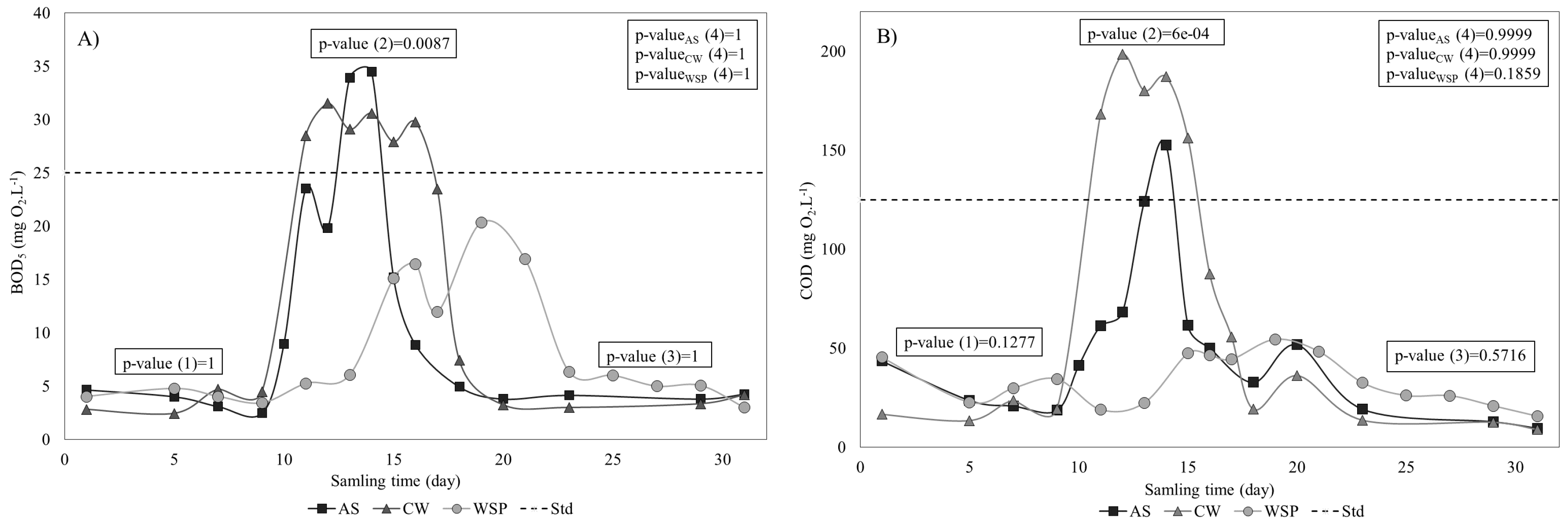
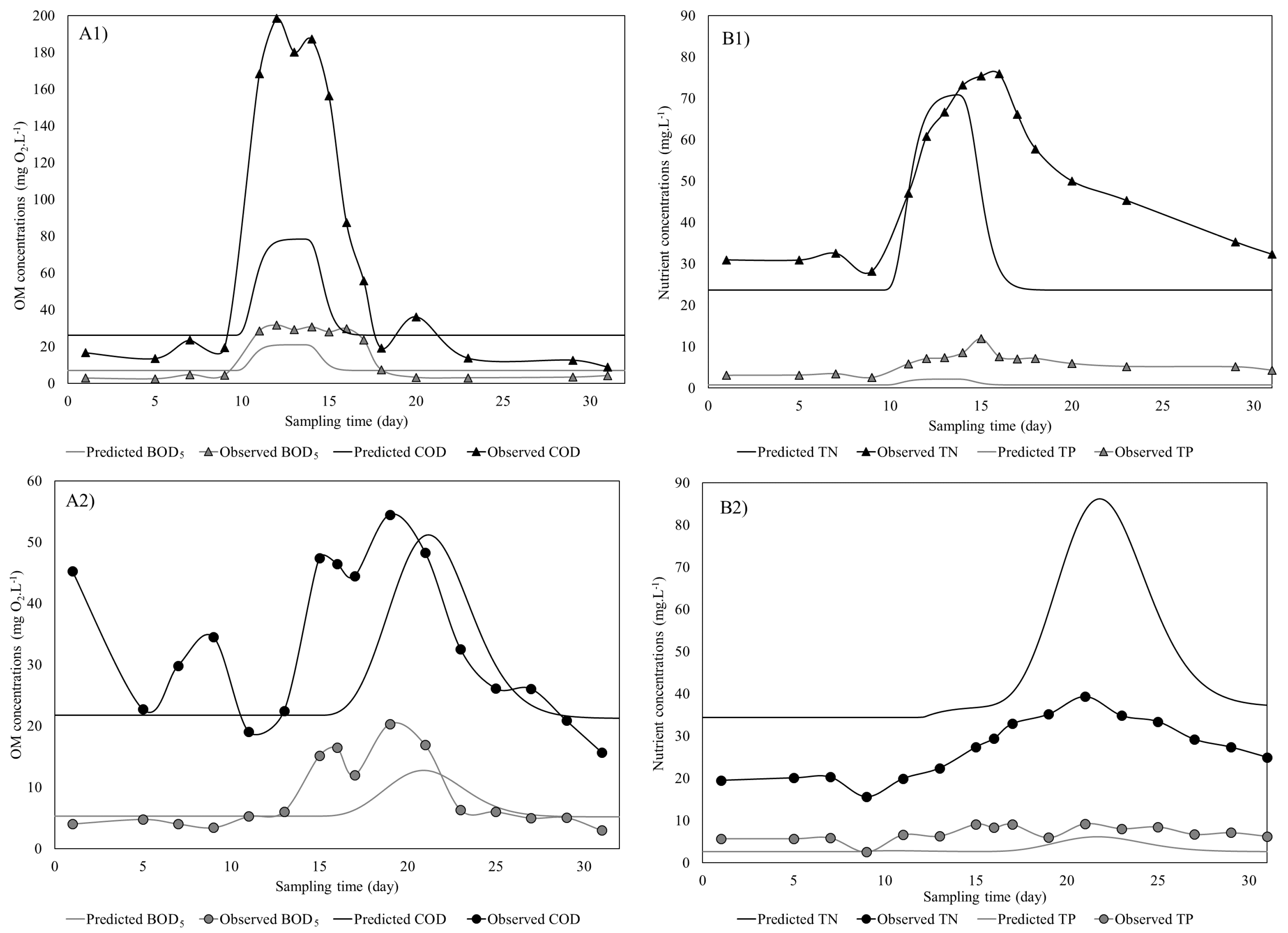
3.1.1. Organic Matter Removal

The organic matter (OM) effluent concentrations of the systems during the peak load scenario are demonstrated with the p-values of the statistical tests in Figure 2. In general, the three systems reacted in analogous patterns before and after the disturbance (high p-values), with high removal efficiencies, around 96% for BOD5 and 90% for COD. Conversely, during the disturbance, their performances were different. This fact was indicated by the low p-values of second hypothesis test, 0.0087 for BOD5 and 0.0006 for COD. While the recovery period of CWs was 7 days for BOD5 and 6 days for COD, this duration in AS systems was around four days when their removal efficiencies dropped to around 90% for BOD5 and 70% for COD. The decrease in effluent quality in these two systems caused the violation of the discharge standard according to the Flemish Environmental Legislation [28]. Meanwhile, WSPs maintained acceptable OM concentrations in the effluent with around six days of recovery time. Compared to the initial values, the OM concentrations at the end phase were relatively similar, as supported by high p-values of the fourth test, except for the case of COD in the pond systems.

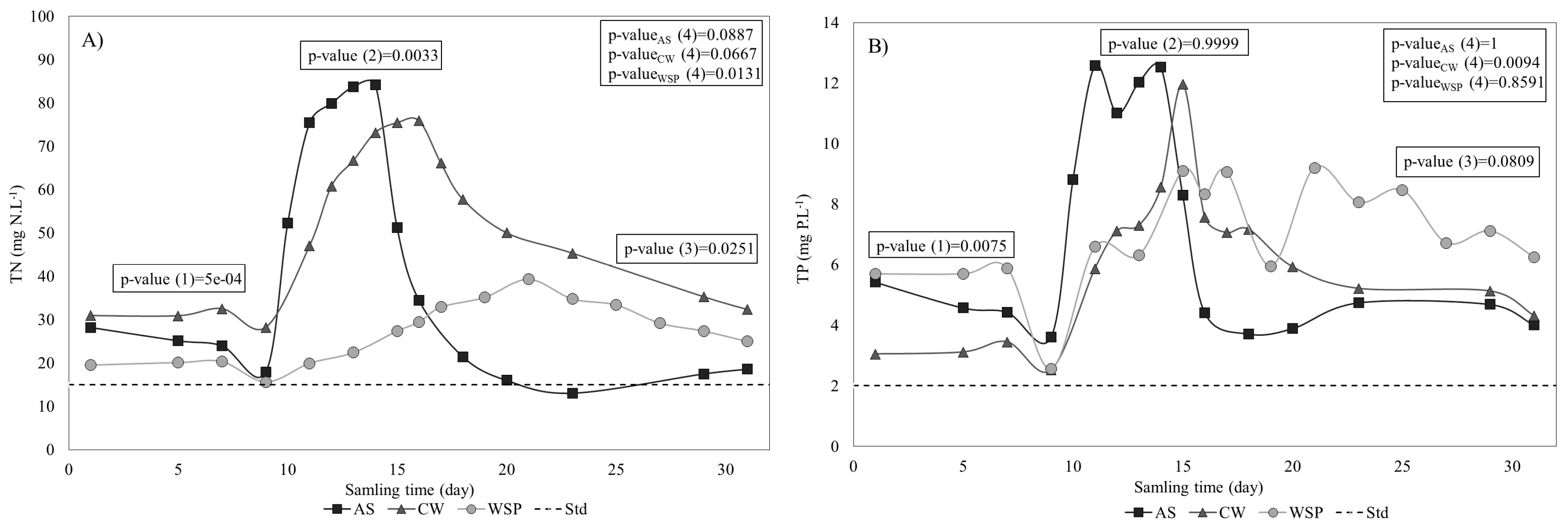
3.1.2. Nutrient Removal

The three systems performed differently regarding nutrient removal, as demonstrated by low p-values of hypothesis tests one to three (Figure 3). Regarding the N removal during the first phase, the pond systems had the best performance with above 51% TN removal in average while wetlands could reach only 22% TN removal. This result is opposite for P removal in which the efficiency of CWs was double that of WSPs, 49% and 24% in average, respectively. During the disturbance, although AS maintained low nutrient removal efficiencies, around 40% for N and 32% for P, it was able to recover within only 6 days after its peak started. Meanwhile, despite higher removal efficiencies obtained in natural systems, such as 70% for N in ponds and 50% for P in both systems, their nutrient concentrations were still higher than their initial concentrations at the end of the predetermined second phase. Indeed, except for P removal in the pond systems, the p-values of two natural systems in the fourth test were low compared to the p-values of AS systems. As the effluents of all three systems exceeded the threshold of the effluent nutrient discharge, a further nutrient treatment is required.

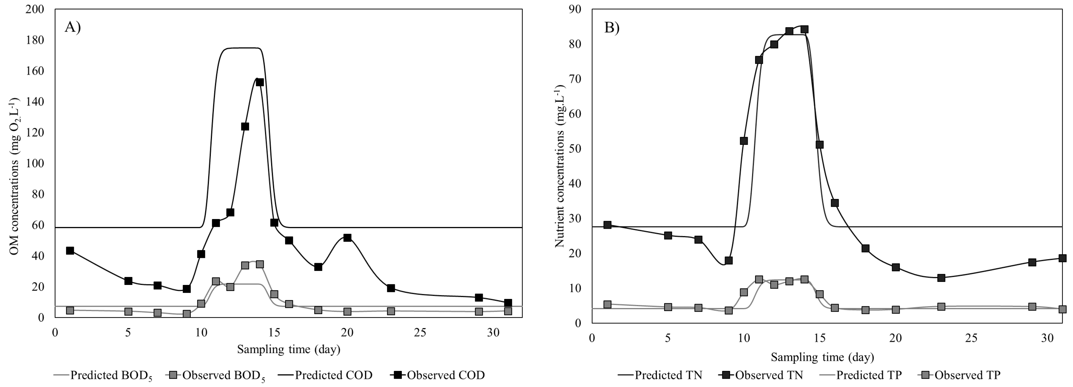
3.2. Model Applicability

3.2.1. Activated Sludge Systems

To predict the performance of the systems during the disturbance, plug flow models were built on the data collected from the preliminary period. More specifically, the removal rates of AS systems were determined, based on first-order kinetic models, which were then applied to simulate the effluent concentrations at the peak scenario. As illustrated in Figure 4, the models predicted relatively precisely the efficiency of AS systems, except for the overestimation of COD removal efficiency. Interestingly, the observed peaks started around half a day earlier than their predictions in all cases.

3.2.2. Natural Systems

In contrast to the agreement between the observed performance of AS and the outputs of the plug flow models, the natural systems showed lower efficiency than the model prediction, except for the case of TN effluent concentrations of WSPs (Figure 5). Indeed, the effluent concentrations were underestimated by around 1.5 times for BOD₅ and 2.5 times for COD in wetland systems. The TP removal efficiency was also higher than its expectations in both systems. Especially worth noting is that their peak periods started earlier and lasted longer than the predictions. For instance, the peak started one day earlier in CWs and it took nine days to reduce to initial effluent concentration of OM and more than 31 days in case of nutrients. In case of WSPs, most effluent peaks started 2.5 days earlier and their TN effluent concentrations remained higher than their initial values until the last day of the scenario.

4. Discussion

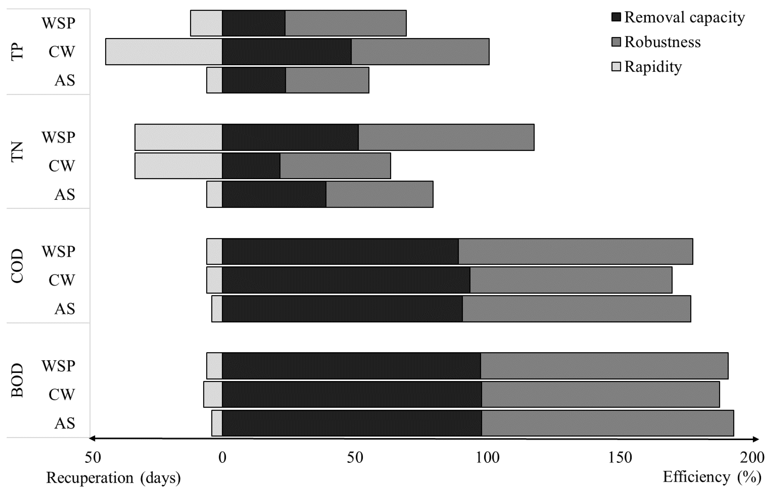
4.1. Removal Capacity

Generally speaking, high OM removal efficiencies were obtained in the three systems during the peak scenario, that is, BOD₅: 87–98% for AS and 94–98% for natural systems, COD: 85–92% for AS and WSPs and 90–95% for CWs. These outcomes of natural systems were relatively higher and fluctuated less than those reported from pilot-scale and full-scale systems, being 75–95% [4,29]. However, nutrient removal efficiencies were relatively low, only 39% of TN and 24% of TP of the influent were removed in AS systems. These relatively low efficiencies might be associated with the shortage of a carbon source in the anoxic reactor, which limited the denitrification process. According to Isaacs and Henze [30], one concern in a combined nitrification-denitrification process is the requirement of a high COD/N ratio, ranging from 5 to 10. Fu, et al. [31] also found that TN removal efficiency decreased by more than 20% when this ratio reduced from 9.3 to 7.0. Indeed, due to high removal efficiency of the first aerobic tank, the COD/TN ratio in the second anoxic tank was only around three. Low P removal could be caused by the out-competition of phosphorus-accumulating organisms (PAOs) in favour of fast-growing heterotrophic bacteria, as a result of the absence of a completely anaerobic phase [32].

Contrary to the AS systems, nutrient removal efficiencies of CWs were relatively high at the beginning of the preliminary period, 43% for TN and 88% for TP. High P removal by CWs can be a result of precipitation and adsorption processes, which are expedited by high Ca²⁺ and Mg²⁺ concentrations. According to the Flemish Environmental Agency in 2015, tap water used for preparing the synthetic wastewater in this experiment is considered as hard water with a hardness from 15–30 °F [33]. However, during the first phase of the disturbance scenario, these removal efficiencies reduced by almost two times, which might be associated with the decline in sorption capacity of the substrate after 6 months of operation [34,35]. As an important process for P removal, sorption is typically defined as a two-phase process in which the adsorption rate is rapid in the first phase and then decelerates as the substrate becomes saturated [36]. The weakness of VF wetland systems in providing suitable conditions for denitrification can explain its low N removal, as in the experiments of Luederitz, et al. [37], the lower N removal was observed in a stratified VF CW compared to horizontal CW.

In case of the pond systems, the N:P ratio of about 4:1 in the synthetic wastewater may contribute to the difference in their nutrient removal efficiencies, 51% for TN and 24% for TP. Since the N:P atomic ratio of both algal and bacterial biomass is around 15:1, the artificial wastewater contained insufficient N to allow complete P removal by assimilation [38]. Together with low water temperature (19 °C), low pH values in both FPs and MPs (only 7.7 and 8.0, respectively), are also limiting factors for phosphate precipitation and ammonia volatilization. Interestingly, in contrast to the decreasing trends in CWs, the pond systems obtained better N removal efficiency in the peak scenario which can be a result of the increase along with time in algal biomass in both FPs and MPs.

4.2. Resilience Capacity

4.2.1. AS Systems

All response curves of AS systems in the second phase had similar shapes. In particular, the effluent concentrations reached a peak within two days after the influent entered the systems, subsequently, they were able to return to initial conditions after four days. During this period, there were two days of excessive OM concentrations in their effluent compared to the standards from the Flemish Environmental Legislation [28]. This quick recovery is because of the relatively high but tolerable influent concentrations which were insufficient to impair the systems. In fact, the food to microorganism ratio during the peak were 0.36 g COD·g⁻¹ VSS·d⁻¹, respectively, which is still in the acceptable ranges for proper functioning, from 0.04 to 1.00 g COD·g⁻¹ VSS·d⁻¹ [12]. The adaptation and recoverability in AS microbial community were indicated via the evolution of biomass concentration and SVI values during the disturbance scenario (Figure 6). After one day of the peak, illustrating the growth of filamentous bacteria, the SVI values increased while the biomass concentrations dropped. However, the increased availability of OM encouraged the N removal efficiency up to 57% in the AS systems. This can be a result of the resilience capacity of ammonia-oxidizing bacteria transforming ammonia into nitrate, which was eventually denitrified because of the increased availability of C-source [39]. This was in line with the research of Thiem and Alkhatib [40], in which the ammonium removal efficiency increased with shock loads.

4.2.2. Constructed Wetlands

Regarding OM removal of CW systems, the removal efficiency was decreased by 20% during the second phase. This result can be associated with their relatively short HRT, which prevented anaerobic processes from degrading slowly biodegradable particulate COD while readily biodegradable organics can be rapidly oxidized under aerobic conditions in VF CWs [41]. Indeed, major OM removal occurred in the first 10–20 cm of VF CW where aerobic conditions are dominant with high microbial density [42]. This fact led to the violation of the effluent discharge during the whole period.

The effects of nutrient shock loads on wetlands were displayed more obvious, in which CWs were not able to return to their initial conditions within 31 days. More importantly, their nutrient effluent levels were even higher than those in the influent were. This outcome might be due to nitrate accumulation and phosphate buffering capacity. Particularly, nitrate accumulation is an inevitable output of the lack of carbon source, which promote nitrification but constrain denitrifying bacteria [43,44]. Regarding phosphorus removal, based on the balance between adsorption and desorption, the equilibrium of its concentrations between the substrate porewater and the liquid phase was maintained [45]. As a result, when the systems reapplied the initial lower-strength wastewater after the second phase, more phosphate desorbed into liquid phase to generate new equilibrium, leading to higher TP concentrations in the effluent.

4.2.3. Waste Stabilization Ponds

The pond treatment systems indicated their high robustness against the organic shock load. The effluent COD concentrations at the end of the scenario were lower than they were at the beginning, leading to a low p-value in the fourth test of 0.1859. More importantly, despite long HRT, the pond systems proved their capacity to recover in a timely manner of around 6 days. However, for removing N, the systems needed more time to recover, although they were able to maintain a low TN level of around 30 mg N·L⁻¹. This result can be associated with the increase of C-source in the influent, which enables the denitrification process. Likewise, the systems also acquired a higher efficiency of P removal during the second phase as the result of a new equilibrium between the solid and liquid phase P concentrations.

4.3. System Applicability

One of the main purposes of this study was to investigate the applicability of the three systems to deal with a shock load scenario with specific interest in both removal efficiency and resilience. While the former can be simply withdrawn from the removal efficiencies of the systems, their resilience capacity is comprised of several characteristics, that is, robustness, redundancy, resourcefulness and rapidity [46]. In our experiments, two of them were illustrated: (1) the robustness representing the ability of a system to withstand disruptions without suffering loss of function; and (2) the rapidity demonstrating the capacity to recover in a timely manner [46]. These characteristics were represented respectively as the height and length of the peaks in Figure 2 and Figure 3. Figure 7 provides a comparative graphical overview of these removal and resilience capacities.

While the OM removal capacities of all three systems are relatively analogous, WSPs showed a better ability to replace AS systems than CWs when dealing with organic shock loads. For example, in contrast to excessive OM concentrations in the effluent discharge of CWs, WSPs were able to comply with the threshold standard. Moreover, they also appeared with higher robustness and rapidity in the case of nutrient removal. While CWs required around two weeks to return to their initial nutrient removal efficiency, WSPs needed only about one week. It is worth noting that it was reported by Greenway and Woolley [47] that effective long-term phosphorus removal was not able to be achieved due to the release in wetland nutrient cycle via desorption process. This process induced a decrease in the nitrogen removal efficiency of the wetland systems in the study of Kumwimba, et al. [48]. In fact, we observed also the decrease of phosphorus removal from 88% in the preliminary period to 45% during the peak scenario in our experiment via this release process. Conversely, this long-term issue is not observed in the AS or WSP systems.

Economic performance is another crucial aspect that should be considered in terms of the applicability of these systems. While the land area requirement of WSPs are largest (2.5 times higher than that of AS) O&M costs, for example, aeration, mixing and sludge disposal costs, of the mechanical systems can be expensive in a long term. However, Mara [49] emphasized that land requirement should be considered as an investment while O&M costs are permanently vanished on a regular basis. Additionally, according to a life cycle assessment of Garfi et al. [50], the AS was 2–3 times more expensive than the natural-based treatment technologies, regarding both capital cost and O&M cost. Moreover, both natural systems provide many important ecosystem services, such as recreation and education, which have not been thoroughly studied. Since such of these systems are expected to last for 60–70 years, a complete and more thorough economic study which takes into account ecosystem services is necessary to evaluate their practicability.

It should be noted that the performance of the natural systems depends more heavily on environmental conditions compared to the AS systems. On the one hand, higher temperature and intensive solar radiation in tropical countries can substantially increase the removal efficiency of both WSPs and CWs. On the other hand, the daily and seasonally variation of these meteorological variables can lead to the fluctuation in the performance of the natural systems [51,52]. This factor should also be considered in choosing the optimal treatment systems. More importantly, as the performance of the natural systems can be significantly improved as a result of advanced and combined configurations, such as hybrid wetland systems, artificially aerated wetlands and advanced integrated wastewater pond systems [53,54], the choice for optimal configurations should be further investigated.

4.4. Model Evaluation

First-order models were applied to a better description of the responses of the three systems during the shock loads, from that we were able to generate a high cost-effective sampling campaign which was able to provide scientifically sound outputs. In fact, these models predicted relatively precisely the effluent curves of AS systems but not in case of the natural systems. Since the hydraulic flow of these two systems is normally non-ideal due to short-circuiting and dead zones, the applicability of the first-order models is relatively limited [55]. This issue was demonstrated via the difference between the starting time of predicted and observed peaks, one day for CWs and 2.5 days for WSPs (Figure 5). Moreover, the kinetic rate of first-order models is assumed to be constant but, in practice and our experiments, it was not [56]. For example, during the second phase, the increase of TN removal rate of WSPs supported them to maintain low TN level in the effluent, leading to the overestimation of the model predictions. Since a model can be applied in multiple steps in the long lifespan of these systems, such as detailed design, process optimization, performance analysis and plant upgrade, a more sophisticated mechanistic model can be a good alternative.

5. Conclusions

• The removal efficiencies and resilience capacities of conventional activated sludge (AS), constructed wetland (CW) and waste stabilization pond (WSP) systems were illustrated via 210 days of experiments with 31 days of the shock load scenario.
• To design a better cost-effective sampling campaign, a meticulous strategy of experimentation was conducted. While preliminary runs and preliminary models showed their benefits in stabilizing the systems and predicting the possible results, hypothesis testing and power analysis ensured adequate sample size as well as statistically and practically meaningful outcomes in this comparison experiment.
• The three systems appeared to have a relatively similar capacity for purifying organic matter (OM) with high removal efficiencies, exceeding 90% but their modest nutrient removal efficiency suggested a necessity for further treatment.
• Regarding resilience capacity, compared to wetland systems, the pond treatment systems proved to be superior to replace AS in dealing with a shock load. Particularly, WSPs represented quicker recovery after the shock load, potentially due to a higher hydraulic retention time. From these perspectives and economic point of view, WSPs are recommended as a more attractive alternative for AS.
• However, land area requirement is a bottleneck for the applicability of a pond treatment system. Hence, when land occupation is the major concern, CWs can be a viable alternative of AS.

References

1. Verstraete, W.; Vlaeminck, S.E. Zerowastewater: Short-cycling of wastewater resources for sustainable cities of the future. Int. J. Sustain. Dev. World 2011, 18, 253–264. [Google Scholar] [CrossRef]
2. UN Water. Tackling a Global Crisis: International Year of Sanitation 2008. Available online: http://www.wsscc.org/fileadmin/files/pdf/publication/IYS_2008_tackling_a_global_crisis.pdf (accessed on 23 April 2016).
3. Von Sperling, M. Comparison among the most frequently used systems for wastewater treatment in developing countries. Water Sci. Technol. 1996, 33, 59–72. [Google Scholar]
4. Muga, H.E.; Mihelcic, J.R. Sustainability of wastewater treatment technologies. J. Environ. Manag. 2008, 88, 437–447. [Google Scholar] [CrossRef] [PubMed]
5. Ayyub, B.M. Systems resilience for multihazard environments: Definition, metrics and valuation for decision making. Risk Anal. 2014, 34, 340–355. [Google Scholar] [CrossRef] [PubMed]
6. Schoen, M.; Hawkins, T.; Xue, X.; Ma, C.; Garland, J.; Ashbolt, N.J. Technologic resilience assessment of coastal community water and wastewater service options. Sustain. Water Qual. Ecol. 2015, 6, 75–87. [Google Scholar] [CrossRef]
7. Qureshi, N.; Shah, J. Aging infrastructure and decreasing demand: A dilemma for water utilities. J. Am. Water Works Assoc. 2014, 106, 51–61. [Google Scholar] [CrossRef]
8. Bettini, Y.; Brown, R.; de Haan, F.J. Water scarcity and institutional change: Lessons in adaptive governance from the drought experience of Perth, Western Australia. Water Sci. Technol. 2013, 67, 2160–2168. [Google Scholar] [CrossRef] [PubMed]
9. Kenward, A.; Yawitz, D.; Raja, U. Sewage Overflows from Hurricane Sandy; Climate Central: Princeton, NJ, USA, 2013. [Google Scholar]
10. The Organisation for Economic Co-operation and Development (OECD). Test No. 303: Simulation Test—Aerobic Sewage Treatment—A: Activated Sludge Units; B: Biofilms; OECD Publishing: Paris, France, 2001. [Google Scholar]
11. Wuhrmann, K. Nitrogen removal in sewage treatment process. Verh. Int. Ver. Limnol. 1964, 15, 580–596. [Google Scholar]
12. Metcalf; Eddy; Burton, F.L.; Stensel, H.D.; Tchobanoglous, G. Wastewater Engineering: Treatment and Reuse; McGraw-Hill Education: New York, NY, USA, 2003; p. 1819. [Google Scholar]
13. Sun, G.Z.; Austin, D. Completely autotrophic nitrogen-removal over nitrite in lab-scale constructed wetlands: Evidence from a mass balance study. Chemosphere 2007, 68, 1120–1128. [Google Scholar] [CrossRef] [PubMed]
14. Tang, X.Q.; Huang, S.L.; Scholz, M.; Li, J.Z. Nutrient removal in pilot-scale constructed wetlands treating eutrophic river water: Assessment of plants, intermittent artificial aeration and polyhedron hollow polypropylene balls. Water Air Soil Pollut. 2009, 197, 61–73. [Google Scholar] [CrossRef]
15. Mara, D.D. Domestic Wastewater Treatment in Developing Countries; Earthscan Publications: London, UK, 2004. [Google Scholar]
16. Ho, L.T.; Van Echelpoel, W.; Goethals, P.L.M. Design of waste stabilization pond systems: A review. Water Res. 2017, 123, 236–248. [Google Scholar] [CrossRef] [PubMed]
17. World Health Organization (WHO). Wastewater Stabilization Ponds: Principles of Planning and Practice; WHO: Geneva, Switzerland, 1987. [Google Scholar]
18. Von Sperling, M. Waste Stabilisation Ponds; IWA Publishing: London, UK, 2007. [Google Scholar]
19. American Public Health Association (APHA). Standard Methods for the Examination of Water and Wastewater; APHA: Washington, DC, USA, 2005. [Google Scholar]
20. Rousseau, D.P.L.; Vanrolleghem, P.A.; De Pauw, N. Model-based design of horizontal subsurface flow constructed treatment wetlands: A review. Water Res. 2004, 38, 1484–1493. [Google Scholar] [CrossRef] [PubMed]
21. Reichert, P. Aquasim—A tool for simulation and data analysis of aquatic systems. Water Sci. Technol. 1994, 30, 21–30. [Google Scholar]
22. Dormann, C.F.; McPherson, J.M.; Araujo, M.B.; Bivand, R.; Bolliger, J.; Carl, G.; Davies, R.G.; Hirzel, A.; Jetz, W.; Kissling, W.D.; et al. Methods to account for spatial autocorrelation in the analysis of species distributional data: A review. Ecography 2007, 30, 609–628. [Google Scholar] [CrossRef]
23. Morrell, C.H. Likelihood ratio testing of variance components in the linear mixed-effects model using restricted maximum likelihood. Biometrics 1998, 54, 1560–1568. [Google Scholar] [CrossRef] [PubMed]
24. R Development Core Team. R: A Language and Environment for Statistical Computing; R Foundation for Statistical Computing: Vienna, Austria, 2011; ISBN 3-900051-07-0. [Google Scholar]
25. Pinheiro, J.; Bates, D.; DebRoy, S.; Sarkar, D.; R Development Core Team. nlme: Linear and Nonlinear Mixed Effects Models, R package version 3.1-103; R Foundation for Statistical Computing: Vienna, Austria, 2012. [Google Scholar]
26. Johnson, P.C.D.; Barry, S.J.E.; Ferguson, H.M.; Muller, P. Power analysis for generalized linear mixed models in ecology and evolution. Methods Ecol. Evol. 2015, 6, 133–142. [Google Scholar] [CrossRef] [PubMed]
27. Bolker, B.M. Ecological Models and Data in R; Princeton University Press: Princeton, NJ, USA, 2008. [Google Scholar]
28. VLAREM II. Decision of the Flemish Government of 01/06/95 Concerning General and Sectoral Regulations with Regard to Environmental Issues; Belgian Government Gazette 31/07/95; Vlaamse Milieumaatschappij: Flanders, Belgium, 1995. [Google Scholar]
29. De Assuncao, F.A.L.; von Sperling, M. Influence of temperature and ph on nitrogen removal in a series of maturation ponds treating anaerobic effluent. Water Sci. Technol. 2013, 67, 2241–2248. [Google Scholar] [CrossRef] [PubMed]
30. Isaacs, S.H.; Henze, M. Controlled carbon source addition to an alternating nitrification denitrification waste-water treatment process including biological p-removal. Water Res. 1995, 29, 77–89. [Google Scholar] [CrossRef]
31. Fu, Z.; Yang, F.; Zhou, F.; Xue, Y. Control of cod/n ratio for nutrient removal in a modified membrane bioreactor (MBR) treating high strength wastewater. Bioresour. Technol. 2009, 100, 136–141. [Google Scholar] [CrossRef] [PubMed]
32. Wong, P.Y.; Cheng, K.Y.; Kaksonen, A.H.; Sutton, D.C.; Ginige, M.P. A novel post denitrification configuration for phosphorus recovery using polyphosphate accumulating organisms. Water Res. 2013, 47, 6488–6495. [Google Scholar] [CrossRef] [PubMed]
33. Reichwaldt, E.S.; Ho, W.Y.; Zhou, W.X.; Ghadouani, A. Sterols indicate water quality and wastewater treatment efficiency. Water Res. 2017, 108, 401–411. [Google Scholar] [CrossRef] [PubMed]
34. Dunne, E.J.; Reddy, K.R. Phosphorus biogeochemistry of wetlands in agricultural watersheds. In Nutrient Management in Agricultural Watersheds: A Wetlands Solution; Academic Publishers: Wageningen, The Netherlands, 2005; pp. 105–119. [Google Scholar]
35. He, S.; Bai, S.Y.; Song, Z.X. Regeneration of p-saturated substrates in constructed wetland. Appl. Mech. Mater. 2014, 448–453, 505–508. [Google Scholar] [CrossRef]
36. Vymazal, J. Removal of nutrients in various types of constructed wetlands. Sci. Total Environ. 2007, 380, 48–65. [Google Scholar] [CrossRef] [PubMed]
37. Luederitz, V.; Eckert, E.; Lange-Weber, M.; Lange, A.; Gersberg, R.M. Nutrient removal efficiency and resource economics of vertical flow and horizontal flow constructed wetlands. Ecol. Eng. 2001, 18, 157–171. [Google Scholar] [CrossRef]
38. Redfield, A.C. On the Proportions of Organic Derivatives in Sea Water and Their Relation to the Composition of Plankton; James Johnstone Memorial Volume; University Press of Liverpool: Liverpool, UK, 1934. [Google Scholar]
39. Cho, K.; Shin, S.G.; Lee, J.; Koo, T.; Kim, W.; Hwang, S. Nitrification resilience and community dynamics of ammonia-oxidizing bacteria with respect to ammonia loading shock in a nitrification reactor treating steel wastewater. J. Biosci. Bioeng. 2016, 122, 196–202. [Google Scholar] [CrossRef] [PubMed]
40. Thiem, L.; Alkhatib, E. In situ adaptation of activated sludge by shock loading to enhance treatment of high ammonia content petrochemical wastewater. J. Water Pollut. Control Fed. 1988, 60, 1245–1252. [Google Scholar]
41. Stefanakis, A.I.; Tsihrintzis, V.A. Effects of loading, resting period, temperature, porous media, vegetation and aeration on performance of pilot-scale vertical flow constructed wetlands. Chem. Eng. J. 2012, 181, 416–430. [Google Scholar] [CrossRef]
42. Kadlec, R.H.; Wallace, S. Treatment Wetlands, 2nd ed.; CRC Press: Boca Raton, FL, USA, 2009; p. 1048. [Google Scholar]
43. Kayser, K.; Kunst, S.; Fehr, G.; Voermanek, H. Nitrification in reed beds—Capacity and potential control methods. Water Sci. Technol. 2002, 46, 363–370. [Google Scholar] [PubMed]
44. Faulwetter, J.L.; Gagnon, V.; Sundberg, C.; Chazarenc, F.; Burr, M.D.; Brisson, J.; Camper, A.K.; Stein, O.R. Microbial processes influencing performance of treatment wetlands: A review. Ecol. Eng. 2009, 35, 987–1004. [Google Scholar] [CrossRef]
45. Barrow, N.J. On the reversibility of phosphate sorption by soils. J. Soil Sci. 1983, 34, 751–758. [Google Scholar] [CrossRef]
46. Bruneau, M.; Reinhorn, A. Exploring the concept of seismic resilience for acute care facilities. Earthq. Spectra 2007, 23, 41–62. [Google Scholar] [CrossRef]
47. Greenway, M.; Woolley, A. Constructed wetlands in Queensland: Performance efficiency and nutrient bioaccumulation. Ecol. Eng. 1999, 12, 39–55. [Google Scholar] [CrossRef]
48. Kumwimba, M.N.; Dzakpasu, M.; Zhu, B.; Muyembe, D.K. Uptake and release of sequestered nutrient in subtropical monsoon ecological ditch plant species. Water Air Soil Pollut. 2016, 227, 405. [Google Scholar] [CrossRef]
49. Mara, D.D. Waste stabilization ponds: Past, present and future. Desalin. Water Treat. 2009, 4, 85–88. [Google Scholar] [CrossRef]
50. Garfi, M.; Flores, L.; Ferrer, I. Life cycle assessment of wastewater treatment systems for small communities: Activated sludge, constructed wetlands and high rate algal ponds. J. Clean. Prod. 2017, 161, 211–219. [Google Scholar] [CrossRef]
51. Ho, L.; Pham, D.; Van Echelpoel, W.; Muchene, L.; Shkedy, Z.; Alvarado, A.; Espinoza-Palacios, J.; Arevalo-Durazno, M.; Thas, O.; Goethals, P. A closer look on spatiotemporal variations of dissolved oxygen in waste stabilization ponds using mixed models. Water 2018, 10, 201. [Google Scholar] [CrossRef]
52. Song, Z.; Zheng, Z.; Li, J.; Sun, X.; Han, X.; Wang, W.; Xu, M. Seasonal and annual performance of a full-scale constructed wetland system for sewage treatment in china. Ecol. Eng. 2006, 26, 272–282. [Google Scholar] [CrossRef]
53. Maltais-Landry, G.; Maranger, R.; Brisson, J.; Chazarenc, F. Nitrogen transformations and retention in planted and artificially aerated constructed wetlands. Water Res. 2009, 43, 535–545. [Google Scholar] [CrossRef] [PubMed]
54. Craggs, R.; Park, J.; Heubeck, S.; Sutherland, D. High rate algal pond systems for low-energy wastewater treatment, nutrient recovery and energy production. N. Z. J. Bot. 2014, 52, 60–73. [Google Scholar] [CrossRef]
55. Ariesyady, H.D.; Fadilah, R.; Kurniasih; Sulaeman, A.; Kardena, E. The distribution of microalgae in a stabilization pond system of a domestic wastewater treatment plant in a tropical environment (case study: Bojongsoang wastewater treatment plant). J. Eng. Technol. Sci. 2016, 48, 86–98. [Google Scholar] [CrossRef]
56. Mitchell, C.; McNevin, D. Alternative analysis of bod removal in subsurface flow constructed wetlands employing Monod kinetics. Water Res. 2001, 35, 1295–1303. [Google Scholar] [CrossRef]
Figure 1. Schematic drawing of the three systems at lab scale. Each system was set up in triplicate located in the same room.
Water 10 00328 g001
Figure 2. The OM effluent concentration of the Activated Sludge (AS), Constructed Wetland (CW) and Waste Stabilization Pond (WSP) with the p-value of four hypothetical tests during the peak load scenario ((A): BOD5, (B): COD). The dot line represents the threshold of the effluent discharge according to the Flemish Environmental Legislation.
Water 10 00328 g002
Figure 3. The nutrient effluent concentration of the Activated Sludge (AS), Constructed Wetland (CW) and Waste Stabilization Pond (WSP) with the p-value of four statistical tests during the peak load scenario ((A): TN, (B): TP). The dot line represents the threshold of the effluent discharge according to the Flemish Environmental Legislation.
Water 10 00328 g003
Figure 4. Predicted and observed effluent concentrations of conventional activated sludge (AS) systems during the peak scenario ((A): Organic Matter (OM), (B): nutrients).
Water 10 00328 g004
Figure 5. Predicted and observed effluent concentrations of constructed wetlands (CW) and waste stabilization ponds (WSP) systems during the peak scenario ((A): Organic Matter (OM), (B): nutrients, 1: CW, 2: WSP).
Water 10 00328 g005
Figure 6. The changes of sludge characteristics during the disturbance. The effects of the shock loads on AS microbial community were illustrated via the increase in SVI values and the drop of biomass concentrations (TSS and VSS).
Water 10 00328 g006
Figure 7. Overview of the removal and resilience capacities of the three systems. Their removal capacity (black) and robustness (dark grey) were calculated as averaged removal efficiencies during the first and second phases of the peak scenario. Rapidity (light grey) was the number of days needed for the systems to recover. When this period exceeded 31 days of the scenario, their rapidity was extrapolated from the linear regression of the decreasing pollutant concentrations in the third phase.
Water 10 00328 g007