Dynamic Management of Water Storage for Flood Control in a Wetland System: A Case Study in Texas

Abstract

In this study, we assess the costs and benefits of dynamic management of water storage to improve flood control in a system of wetlands. This management involves releasing water from wetlands ahead of (e.g., a few hours or days before) a rainfall event that is forecasted to produce flooding. Each project site may present different challenges and topographical conditions, however as long as there is a relatively small hydraulic gradient between the wetland water surface and the drainage ditch (e.g., >0.9 m), wetlands can be engineered for the purpose of flood control. We present a case study for a system comprised of four wetland areas encompassing 925 acres in the coastal plain south of Houston, Texas. The benefit–cost analysis shows that, in general, the benefits of wetland ecosystems far surpass the costs of construction and maintenance for all considered periods of analysis and assumed degrees of dynamic management of wetland storage. The analysis also shows that the benefit/cost ratios increase over the period of analysis. Considering flood protection only (e.g., not considering the value of other ecosystem services), as long as dynamic management of wetland storage increases flood protection by about 50% compared to that with no management (e.g., a typical wetland with no controlled release of water), the construction of a wetland system would have a benefit/cost ratio of at least 1.9.

1. Introduction

Multi-mitigation projects within the context of a watershed approach have been receiving increasing attention in the last few decades [1,2]. In the watershed approach, the entire watershed becomes the objective of management so that for example human activities (e.g., land development) upstream can be associated to inundation in a downstream area (e.g., [2]). It has been recognized that within a watershed, wetlands can play a significant role in flood control, while providing other benefits such as creating habitats for flora and fauna, improving water quality, and providing opportunities for recreation and public appreciation (e.g., [3,4,5,6,7,8,9,10,11,12,13,14]). It is recognized that wetlands can help in flood reduction by storing, holding, and percolating water [4,7], however their effectiveness is constrained due to their limited storage capacity and the fact that some or all of this capacity may be occupied when a flood is imminent. The Galloway report [15] suggests that upland wetlands could be effective for containing smaller floods, but decrease in effectiveness for larger floods. One strategy for increasing the effectiveness of wetlands for larger floods could be to release part of the water ahead of (e.g., a few hours or a couple of days before) heavy rainfall so that as much of the wetland volume as possible is made available for flood control.

Many wetlands naturally have a variable hydroperiod, so their function is not necessarily reduced by partial draining. If draining is complete, however, species that require standing water, such as fish, will be eliminated. Moreover, if a wetland is mostly drained to low water levels in anticipation of a storm and the storm does not materialize, the wetland will be at risk of drying out completely in the following days due to natural evapotranspiration. Thus, draining involves some risks, which can be minimized by not draining the wetlands fully, and by draining only when the certainty of rain events is very high, which may be achieved in the best of cases a few hours or days in advance of a predicted storm.

The work presented herein addresses part of a larger topic which is to dynamically manage the water storage of a system of interconnected wetlands for flood reduction. The authors refer to dynamic water storage management as the controlled release of water from wetlands ahead of large storm events that are forecasted to produce flooding. In this way, wetland storage can be made available for the storm event and hence reduce flooding. The design of a wetland involves multiple components such as vegetation selection, soil media improvement, basin size selection, hydrological, sedimentation and topographical considerations, etc. The reader is referred to [16,17,18] for a discussion on the latter considerations. Moreover, a system of interconnected wetlands could consist of any combination of natural wetlands, constructed wetlands, flood control structures, and accidental wetlands. Different engineering and ecological issues would apply for each type of wetland. The scope of this paper is limited to the benefit–cost analysis of dynamic management of water storage in a system of wetlands for improving flood control. This paper is organized as follows. Firstly, the setup of a hypothetical wetland system located on the grounds of the University of Houston Coastal Center is described. Secondly, the hydraulics of the drainage of the hypothetical wetland system are presented. Thirdly, a multi-objective optimization model is combined with the hydraulics model for the optimal selection of piping for the drainage of the wetland system. Fourthly, the benefit–cost analysis is discussed. Finally, the key results are summarized in the conclusion.

2. Case Study

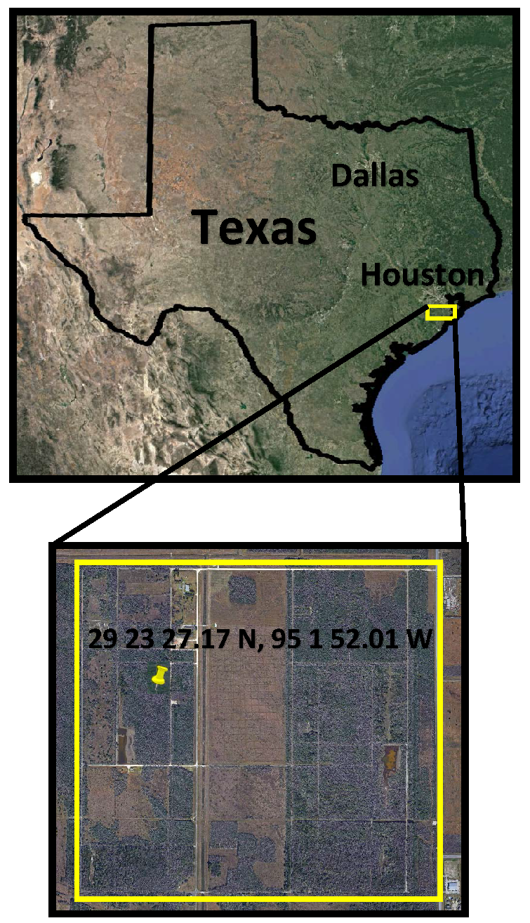
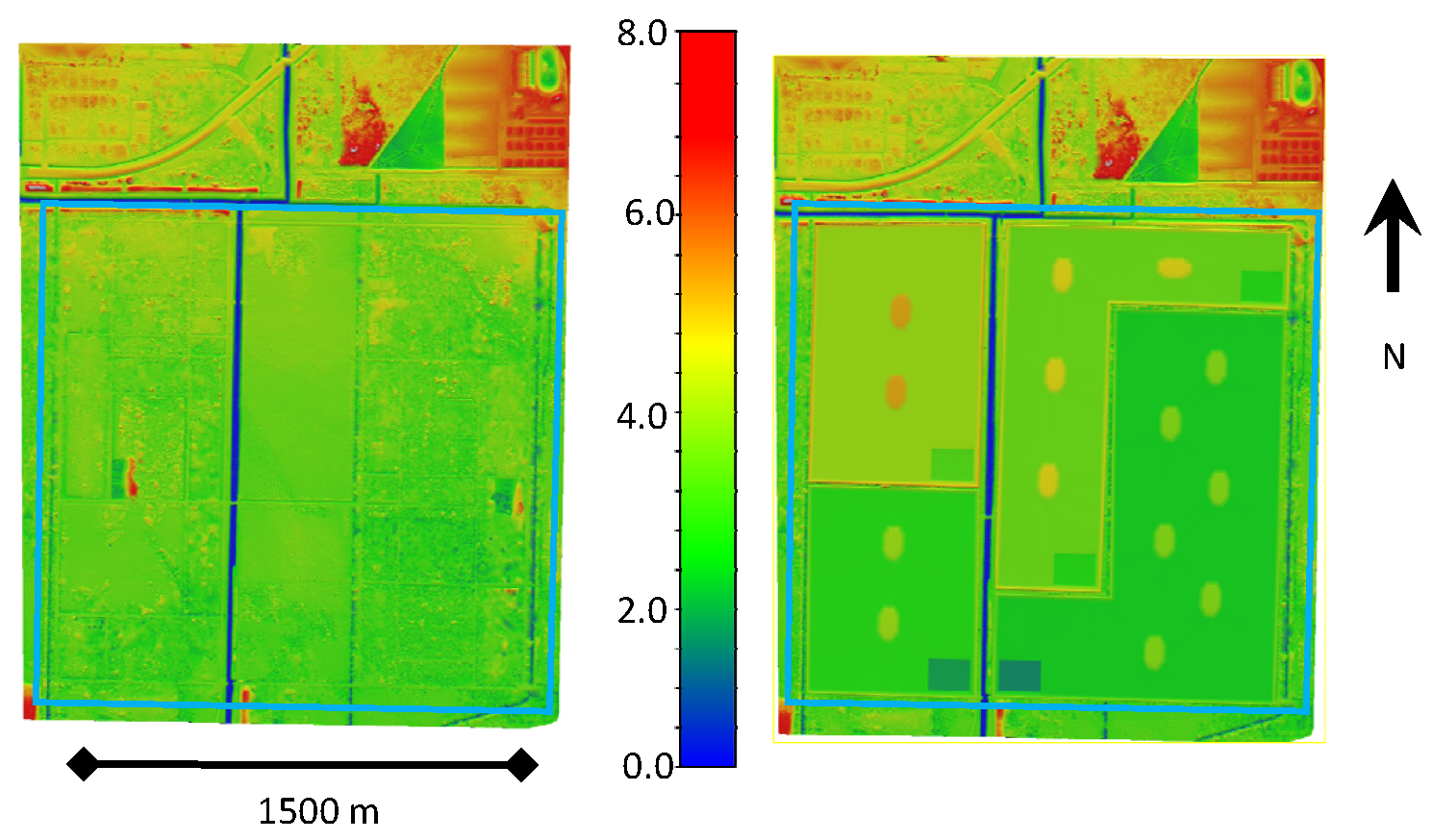
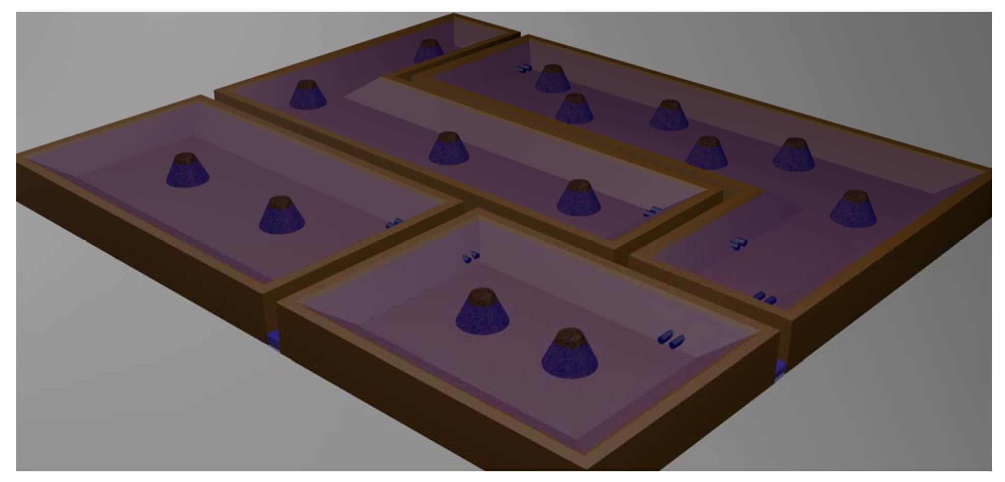
The Coastal Plains in Texas, where the city of Houston and most other densely populated cities in the State are located, encompass about two-fifths of the Texas land area and are essentially flat, low prairies that stretch inland from the Gulf Coast [19]. To show that wetlands can be engineered for flood control even in relatively flat areas, our case study was selected in a coastal plain area. This case study, which is shown in Figure 1, takes place in a 925-acre field station located at the University of Houston Coastal Center (UHCC), 30 km south of metropolitan Houston and 22 km north of the Gulf of Mexico. Water draining from the site enters Highland Bayou, and ultimately flows into Galveston Bay. The 925-acre site was virtually engineered to create four wetlands and their ancillary components (e.g., drainage) as shown in Figure 2. A three-dimensional sketch of the UHCC wetland system after virtual modification is shown in Figure 3.

2.1. Geomatic Considerations

To enable a realistic earthwork grading analysis for the construction of the wetland system in the UHCC, a high-resolution topographic map of the site was derived from a high-resolution terrain model acquired using airborne Light Detection and Ranging (LiDAR), also known as airborne laser swath mapping [20]. The LiDAR data is publicly available through the Texas Natural Resources Information System (https://tnris.org/), and was acquired in 2008 for producing 1-ft elevation contours for Harris County, TX. Although the LiDAR data is almost 10 years old, there have been minimal changes in the UHCC landscape and therefore the model accurately represents existing conditions.

To build a representative wetland water storage system, it was desirable to both maximize the water volume storage of the system, and almost balance the amount of cut and fill required at the site to ensure that all required soil would be available at the site. Therefore, an iterative approach was implemented to alter the landscape to produce the wetlands to fulfill these major criteria. While manually iterated for this demonstration, this analysis could be automated for future applications.

The earthworks required for constructing the UHCC wetland system are shown in

Table 1. Wetland geometric characteristics and earthwork volumes required for constructing each of the wetlands.

Wetland	Bottom Elevation (m)	Water Surf. Elevation (m)	Surface Area (m2)	Storage Volume (m3)	Cut Volume (m3)	Fill Volume (m3)
1	3.6	4.4	972,500	760,000	122,000	69,000
2	4.4	5.2	654,000	515,000	73,400	115,400
3	3.8	4.6	440,000	340,000	178,200	25,500
4	4.8	5.6	554,000	430,000	21,500	180,500

. As shown in this table, the total cut is slightly greater than the total fill, which means that all the fill needed is generated on site.

2.2. Environmental Considerations

What types of wetlands would be available for projects like this, and what are the environmental concerns with respect to using them? A typical urban area is likely to have a mixture of remnant natural wetlands, constructed artificial wetlands meant to mimic natural wetlands, artificial flood control structures such as detention ponds, and “accidental wetlands” that form as an unintended consequence of land use and water infrastructure decisions [21,22]. All of these could be incorporated into an engineered network such as the one described here, but different political and environmental considerations would apply. In particular, the natural and artificial wetlands are likely to have the most ecological value, while being the most politically sensitive and subject to the greatest level of regulation.

All natural systems are inherently variable over time [23]. Shallow depressional wetlands are particularly variable, because their primary source of water is rainfall, which occurs intermittently, and because they are shallow enough that they can dry out completely during periods without rain [24]. This variability is described by the hydroperiod—a record of water depth over time. There is a fundamental ecological distinction between wetlands that retain some water year-round, and those that dry out periodically, because only the former support long-lived aquatic animals such as fish, as well as wetland amphibians and invertebrates, which are important predators [25,26]. Among wetlands that dry out periodically, ones that stay wet for longer periods (a long hydroperiod) can support amphibians and insects with aquatic life stages that require water for weeks or months at a time, and tend to support obligate aquatic plants. At the dry extreme, wetlands that are flooded for only short periods of the year (a short hydroperiod) support primarily facultative wetland animals and plant species that benefit from or can tolerate occasional flooded conditions but do not require them most of the year [27,28,29]. These considerations suggest that intervention in natural and artificial wetlands should be cautious so that the characteristics of the natural hydroperiod are retained. In particular, if a wetland supports fish, it should be drained only partially and only when imminent rainfall is likely to refill the wetland and reduce the risk that it completely dries out. In contrast, the hydroperiods of wetlands that naturally dry out periodically can be manipulated more aggressively in advance of a storm without markedly changing the ecological function of the wetland. Even for temporary wetlands, a dramatic shift in the hydroperiod will lead to a shift in plant and animal composition. The hydroperiod naturally varies among years due to variations in precipitation [30], however, changes to the hydroperiod in a single year (for example due to draining a wetland in advance of a storm that fails to materialize) may not change the long-term ecological function of the wetland as long as the altered hydroperiod does not fall outside the long-term distribution of historical hydroperiods for the area. Most interestingly, because the hydroperiod of detention ponds and accidental wetlands may not match the hydroperiod of natural wetlands in a particular geographic area (in particular, detention ponds are often engineered to dry completely between storms—a very short hydroperiod—and as such provide low ecological function), the possibility exists that extending the hydroperiods of these habitats towards a more natural regime using water control techniques such as that described here would allow these habitats to achieve a higher ecological value than they currently provide. Finally, one of the important ecological “disservices” provided by temporary wetlands to humans is the support of mosquito populations. The ability to control the hydroperiod of a wetland could potentially be used to help control mosquito populations by creating hydrological conditions amenable to native predators of mosquitoes, unsuitable to mosquito larvae, or unsuitable to wetland vegetation preferred by mosquitoes [31,32]. Similarly, freshwater wetlands produce methane, a potent greenhouse gas, and it is possible that the hydroperiod could be manipulated to maximize ecological benefits while minimizing methane production. These considerations are beyond the scope of this paper, but would merit attention in future work to optimize water regulation decisions.

Historically, the Texas coast supported extensive complexes of prairies and depressional wetlands referred to as “potholes” [33]. Potholes filled with water seasonally during periods of heavy rain, and the duration of flooding varied from weeks to months as a function of pothole size and geographic location [33]. Potholes provided habitat for a variety of reptiles, amphibians, mammals, and resident and migratory birds, and also stored vast amounts of water during rainy periods [33]. Because most were not continuously flooded, there is considerable latitude to manage their hydroperiod without markedly altering their ecological function. Depressional wetlands in the United States in general and along the Texas coast in particular have greatly decreased in area over the past century due to a land use change to agriculture and urban sprawl [34,35]. Urban areas in particular have lost surface water features [21]. As a result, both natural habitat and flood protection have been lost. Although depressional wetlands are geographically isolated [34], they are hydrologically connected by surface runoff through intermittently flowing channels during periods of heavy precipitation [36]. Thus, these natural wetlands historically functioned as a connected network of flood retention basins, but not necessarily in a manner that was optimized for flood control.

Historically, the site of our case study (the UHCC) would have been dominated by coastal prairie; today, it is a mixture of prairie and forest. For illustrative purposes, we assumed that the entire site would be available for the purpose of creating a network of artificial wetlands with the primary goal of flood control. The artificial wetlands would provide a variety of additional services beyond flood control, including trapping of sediments and nutrients, and providing habitat for wildlife. If the project sought to create a semi-natural landscape that would balance flood control with these other ecosystem services, the proportion of a site converted to wetlands would probably be closer to the historical value of 30% ([33]). Examining the tradeoffs between these potential services and how this would affect the exact proportion of land devoted to wetlands is beyond the scope of this paper.

2.3. Simulated Scenario

It is clear that each project site may have specific challenges and different topographical conditions, however as long as there is a relatively small hydraulic head (e.g., >0.9 m) between the wetland water surface and the discharge point or drainage ditch, wetlands can be engineered for the purpose of flood control.

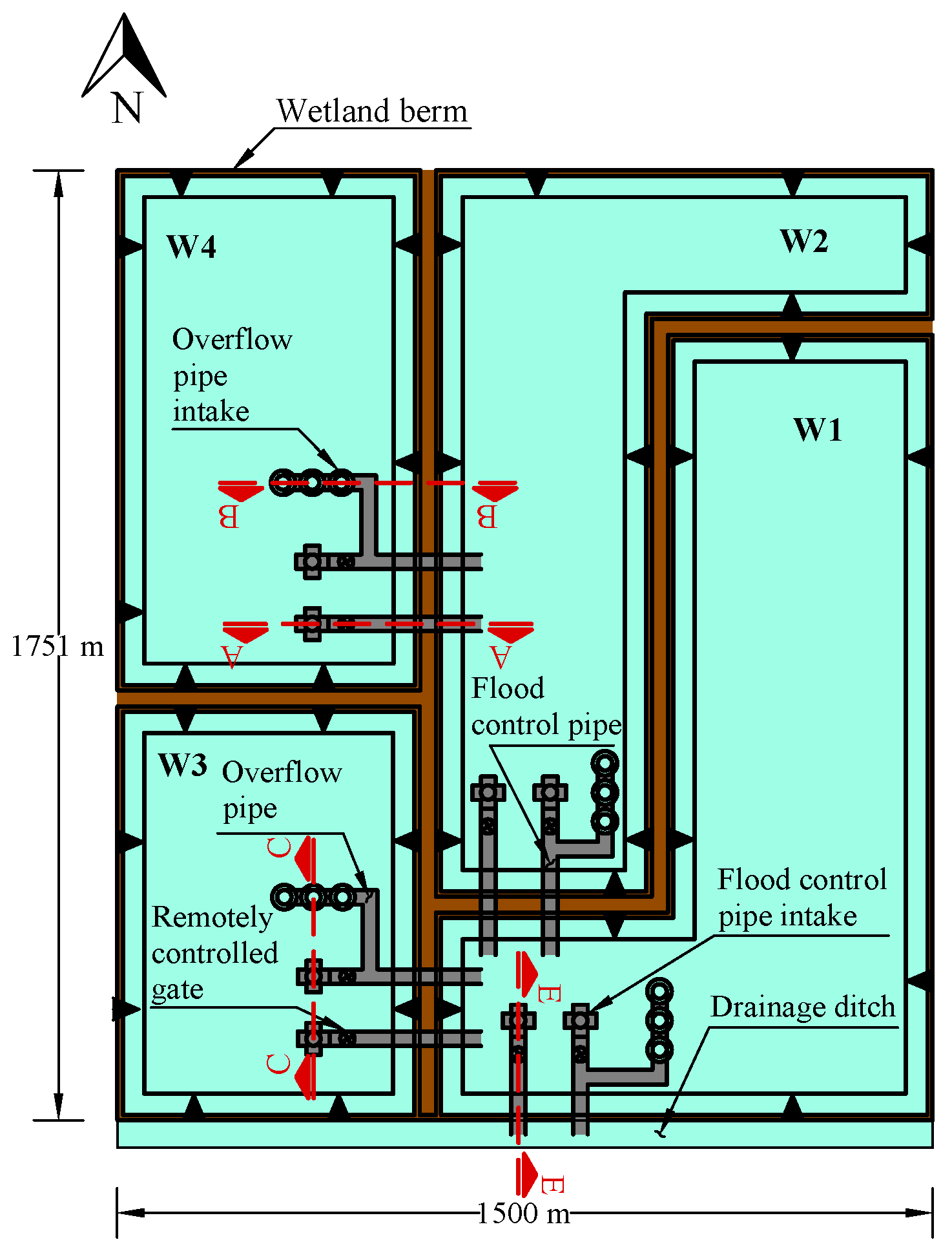
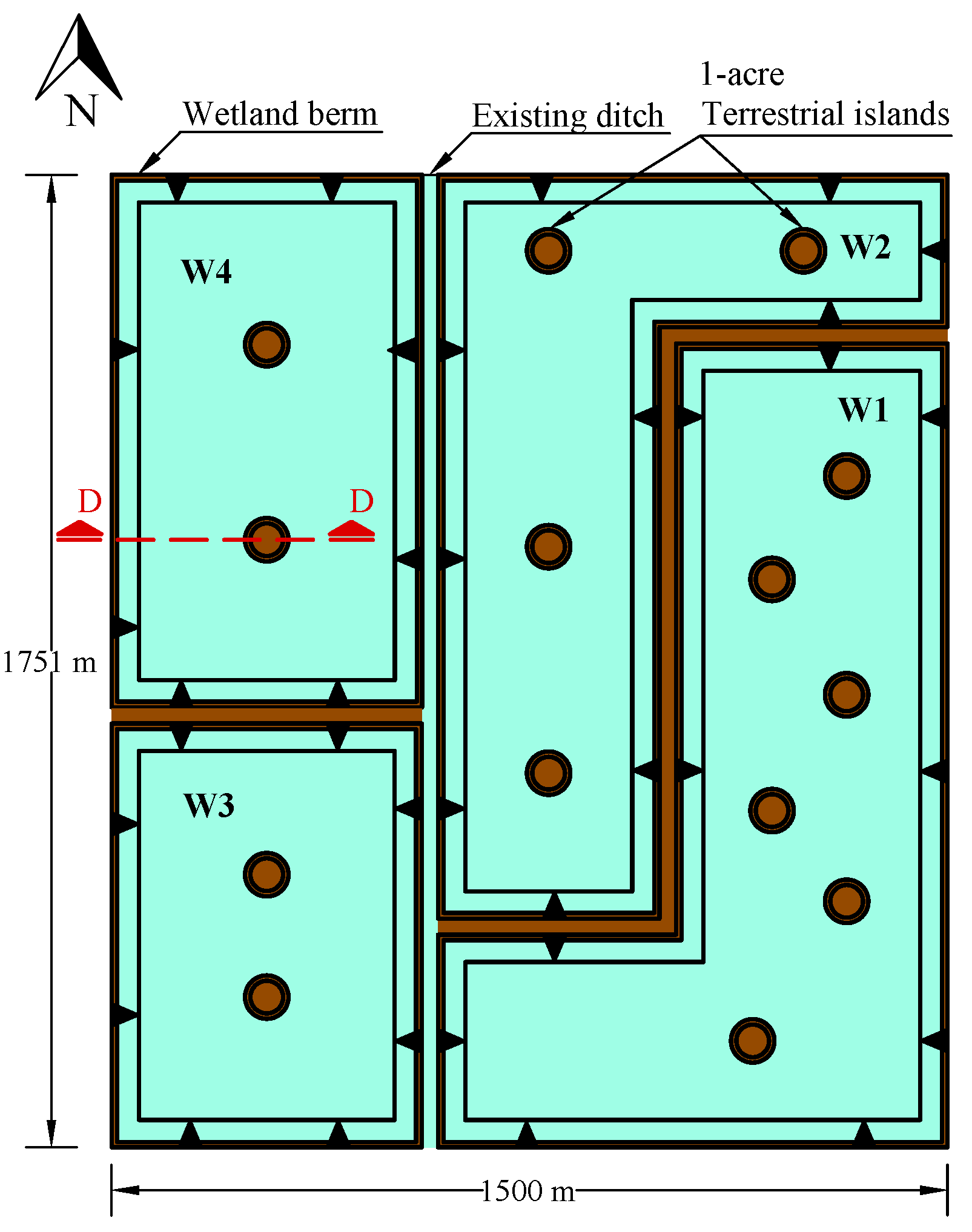
As shown in Figure 4, the simulated scenario assumes that the four interconnected wetlands have a single discharge to the most downstream lateral ditch. Because the edge habitat between the water and terrestrial habitats is ecologically important, we assume that each wetland would have several engineered one-acre islands—in this case these reduce the maximum water volume of the wetlands by 1.5% but provide additional edge habitat and create 14 acres of upland habitats protected by water from terrestrial predators. The plan view of the islands is shown in Figure 5.

Figure 4 depicts the layout of the “flood” and “overflow” pipes as well as the remotely operated gates. The “flood” pipes are intended for releasing water ahead of (e.g., a few hours or days before) a heavy rainfall event that is forecasted to produce flooding. This water release is performed using remotely controlled gates. It is expected that remote operation of gates will be necessary because the use of wetlands for flood control requires a relatively large surface area, necessitating the spread of multiple wetlands over a large geographic area. To make this remote operation of gates/valves possible, a control system similar to the Supervisory Control and Data Acquisition (SCADA) system could be used (e.g., [37]). An “overflow” pipe releases the water that exceeds the maximum water level in the wetland which in this case is 0.15 m below the top of the wetland berm. As can be observed in Figure 4, the “flood” and “overflow” pipes are connected downstream of the respective remotely operated gate. The intake for the “flood” pipe is considered to have a five-way inlet to avoid inlet control. As discussed in [38], inlet control conditions may occur for inlets that significantly restrict the flow. Furthermore, because natural and most artificial wetlands are restricted to shallow water depths and small hydraulic heads (e.g., the difference between upstream water surface elevation and downstream discharge elevation), a single intake for both pipes (“flood” and “overflow”) would not work for shallow water depths. Thus, a separate intake is used for the “flood” and “overflow” pipes.

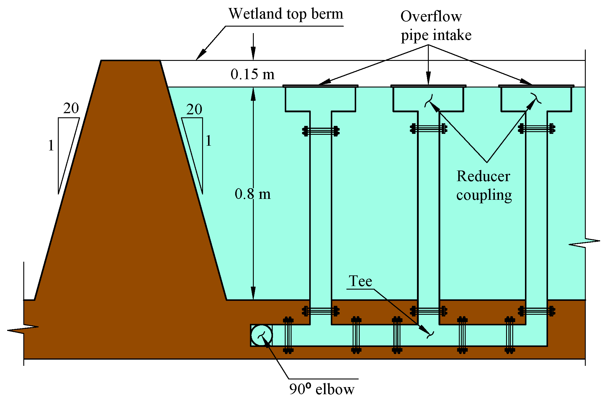
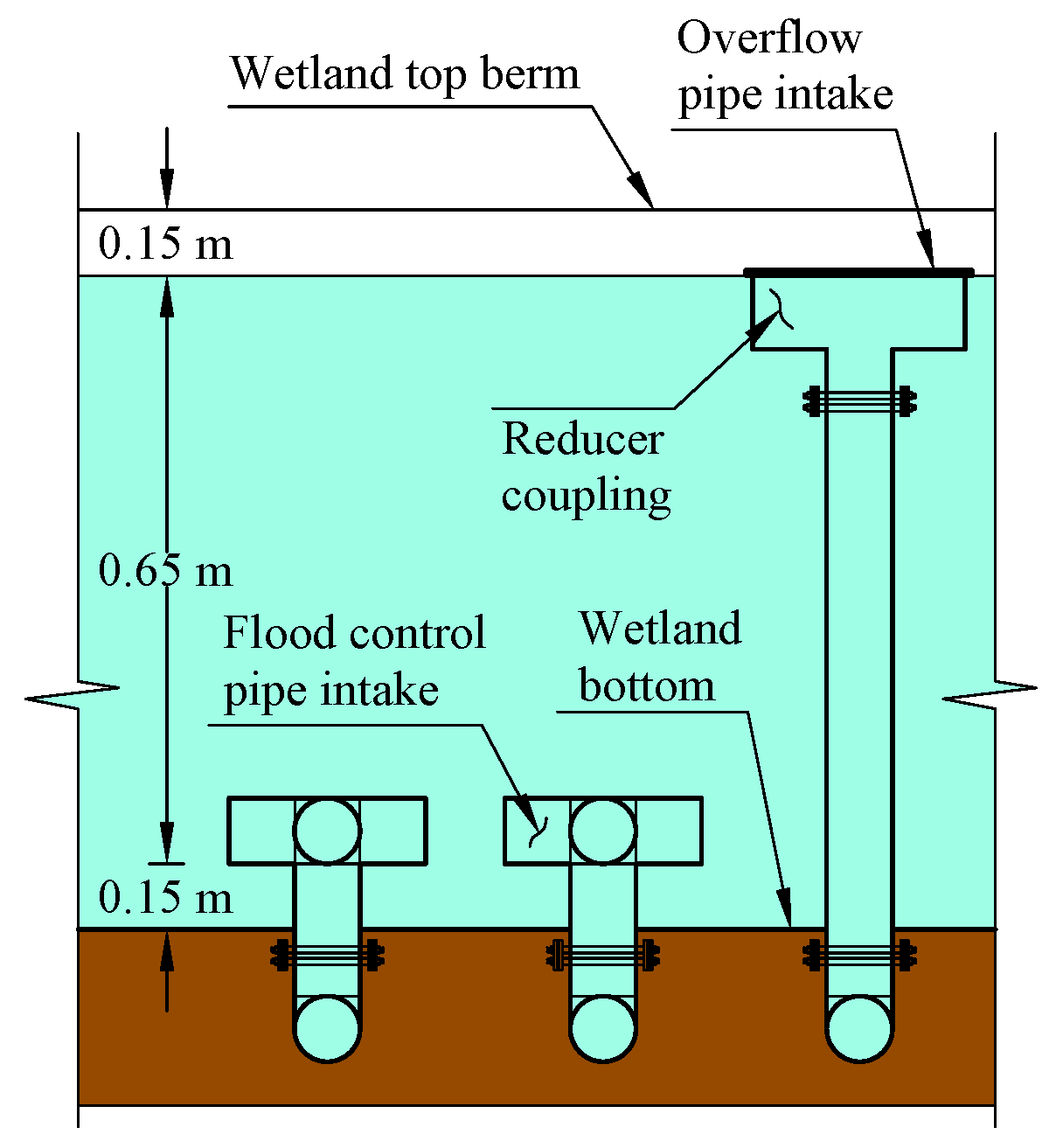
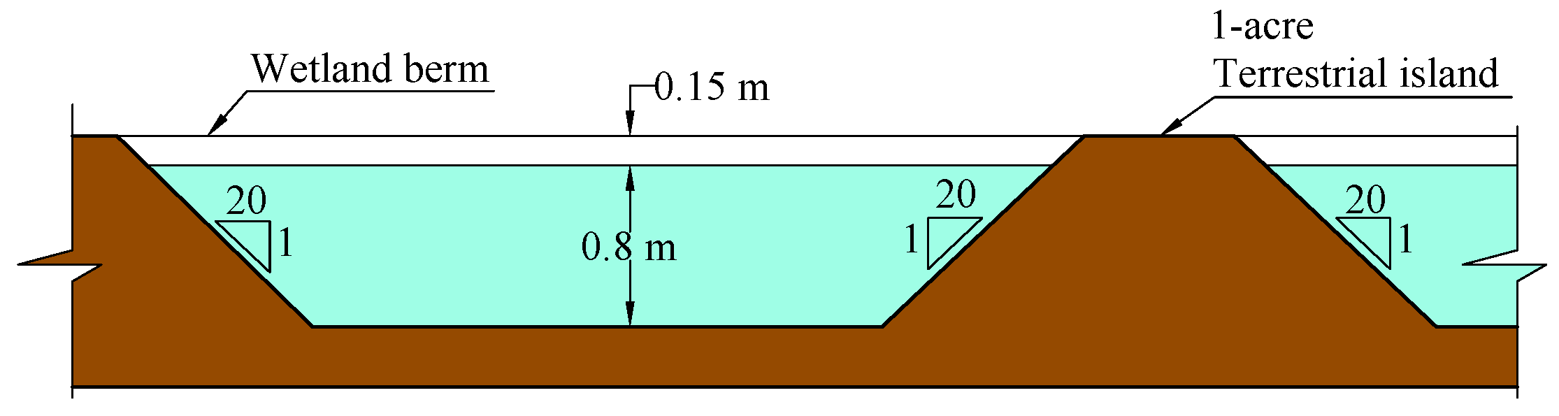
The wetland overflows are cascaded from the most upstream wetlands to the most downstream. To provide further details on the wetland drainage, Figure 6, Figure 7, Figure 8, Figure 9 and Figure 10 show sectional views A-A, B-B, C-C, D-D and E-E, respectively, indicated in the above plan views (Figure 4 and Figure 5). Figure 6 shows the intake for the “flood” pipe. As can be observed in this figure, the invert elevation of the intake for the flood pipe is 0.15 m above the wetland bottom, which prevents the wetland from draining completely even if the remotely controlled drainage system is set to release as much water as possible. If the wetland does not receive new water inputs, however, it will then be vulnerable to drying out completely due to evapotranspiration. Also, as observed in Figure 6, a sediment trap with a minimum surface area of 25 m${}^2$ and a depth of 0.15 m below the wetland bottom is located right upstream of the flood control pipe intake. The sediment trap should be accessible to heavy machinery so that it can periodically be scraped out and accumulated sediment moved to a suitable disposal site—either to a berm or (if it is heavily polluted) a landfill. The benefit of the sediment trap is to reduce clogging of the flood control pipe intake. Another benefit is improved water clarity and (if the sediment is polluted) improved water quality. Figure 7 shows the intake for the “overflow” pipe. As shown in this figure, the invert level of the intake for the overflow pipe is 0.15 m below the wetland top berm. Figure 8 shows the intake for the “flood” and “overflow” pipes in a perpendicular view to that of sections A-A (Figure 6) and B-B (Figure 7). This figure also shows the elevations of the inverts of the intakes of both pipes, and the bottom elevation of the “flood” and “overflow” pipes. In addition, Figure 9 shows the side view of the one-acre terrestrial island while as Figure 10 shows the side view of flow discharge from the downstream wetland to the drainage ditch.

The data for the simulated scenario are presented below.

• The tailwater elevation for the flood pipe(s) at wetland 1 is below the outlet invert of the flood pipe(s).
• The drop height between the inlet and outlet inverts ($LS$) is set to 0.5 ft (0.15 m) for all flood pipes.
• The length (L) for all “flood pipes” is 400 ft (121.9 m).
• The soil cover height over the pipe crown ($h_p$) is set to 1.25D, where D is the pipe diameter.
• The surface area ($Aw$) values of wetlands 1 to 4 are 240.31 acres (972,500 m${}^2$), 161.61 acres (654,000 m${}^2$), 108.73 acres (440,000 m${}^2$), and 136.90 acres (554,000 m${}^2$), respectively.
• The vertical distance from the invert of the five-way flood pipe intake to the bottom of the wetland ($h_s$) is set to 0.5 ft (0.15 m).
• The Manning’s roughness (n) for all “flood pipes” is set to 0.009.
• The entrance loss coefficient ($k_e$) for the intake of all “flood pipes” is set to 0.8.
• The initial water depth measured above the invert of the five-way flood pipe intake (h) for all wetlands is set to 2 ft (0.61 m).

2.4. Hydraulics of Simulated Scenarios

The water balance equations for the four-wetland system (i = 1, 2, 3 and 4) can be written as:

$$\sum I_i-\sum O_i=A{w}_i\left(\frac{\mathsf{\Delta }{h}_i}{\mathsf{\Delta }t}\right)$$

(1)

where $\sum I_i$ and $\sum O_i$ are the sums of inflows and outflows at wetland i, respectively, $Aw$ is the wetland surface area, t is time, and h is the wetland water depth measured above the invert of the flood pipe intake. To release large volumes of water in a short time period, parallel pipes of the same diameter may be needed in a wetland. Herein, the number of parallel pipes at wetland i is denoted as $m_i$. In a similar way to [38], the energy equation for the four flood pipes (i = 1, 2, 3 and 4) can be written as:

$$H{W}_i+L{S}_i=h_{o_i}+\frac{A_{c_i}^3}{2T_{c_i}{A}_i^2}\left[1+k_{e_i}+\frac{K_u{n}^2{L}_i}{R_i^{1.33}}\right]$$

(2)

where $HW$ is the headwater depth above the entrance invert, $LS$ is the drop height between the inlet and outlet culvert inverts, $k_e$ is the entrance loss coefficient, n is the Manning’s roughness coefficient, L is the pipe length, R is the pipe hydraulic radius, Q is the flow discharge, A is the cross-sectional area of the pipe, $K_u$ is a constant equal to 29 in English units (19.63 in SI), $A_c$ is the critical flow area, and $T_c$ is the critical flow surface width. $h_{o_i}$ (i = 1, 2, 3 and 4) is given by:

$$h_{o_1}=max(\frac{h_{c_1}+D_1}{2},TW)$$

(3)

$$h_{o_2}=max(\frac{h_{c_2}+D_2}{2},H{W}_1)$$

(4)

$$h_{o_3}=max(\frac{h_{c_3}+D_3}{2},H{W}_1)$$

(5)

$$h_{o_4}=max(\frac{h_{c_4}+D_4}{2},H{W}_2)$$

(6)

where $h_c$ is the critical depth, D is the pipe diameter, and $TW$ is the tailwater depth above the outlet invert. In a similar way to [38], Equation (2) is solved for the respective critical depths, which in turn can be used for calculating the outflows in pipes 1 to 4 using the following equation:

$$Q_i=\sqrt{g{A}_{c_i}^3/T_{c_i}}$$

(7)

It is noted that the total outflow at wetland i ($\sum Q_i$) would be given by $m_i{Q}_i$. Once the outflows have been determined, the water depth in wetlands 1 to 4 at the new time can be updated as follows:

$$h_1^{t+1}=h_1^t+\frac{\mathsf{\Delta }t}{A{w}_1}(\sum Q_2^t+\sum Q_3^t-\sum Q_1^t)$$

(8)

$$h_2^{t+1}=h_2^t+\frac{\mathsf{\Delta }t}{A{w}_2}(\sum Q_4^t-\sum Q_2^t)$$

(9)

$$h_3^{t+1}=h_3^t+\frac{\mathsf{\Delta }t}{A{w}_3}(-\sum Q_3^t)$$

(10)

$$h_4^{t+1}=h_4^t+\frac{\mathsf{\Delta }t}{A{w}_4}(-\sum Q_4^t)$$

(11)

The above process is repeated for the entire simulation period.

2.5. Time Step Convergence of Wetland Drainage Model

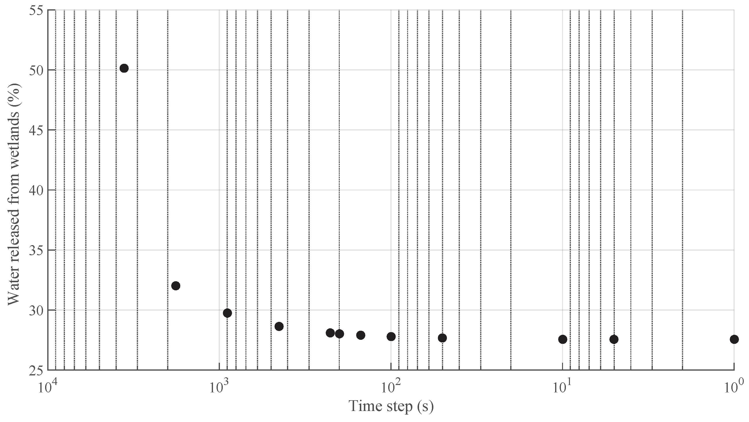
Various time steps, ranging from 1 s to 3600 s, were used for analyzing the time step convergence of the wetland drainage model. In the simulations, the releasing time was fixed to 3 h and the number of $24{}^{″}$ (610 mm) pipes in wetlands 1 to 4 were fixed to 3, 1, 1, and 1, respectively. This arrangement corresponds to one of the set of optimal solutions obtained using the optimization model described in Section 2.6. The results of time step convergence for the percentage of water released from the wetlands is shown in Figure 11. As can be observed in this figure, the model achieves time step convergence for $\mathsf{\Delta }t$ of about 200 s or smaller. For the remaining simulations of this paper, a time step of 100 s was used to ensure that the results are time-step independent.

2.6. Optimal Number of Pipes for Each Wetland

The non-dominated sorting genetic algorithm [39] was used as the optimization model for determining the optimal diameters of the flood pipes. A population of 100 and a generation of 500 was used in the case study. Other parameters, such as crossover rate, were selected to be the same as in the study of [39]. Two objectives were considered in the optimization. The first objective was to minimize the cost of the flood pipes and automated gates. The second one was to maximize the conveyance capacity of the flood pipes. It is clear that these objectives conflict with each other and the optimal trade-off is a desired result for the design. The wetland hydraulics model, which was described earlier, was used for evaluating the objectives in the optimization model. In the optimization model, the number of $24{}^{″}$ flood pipes for the four wetlands are the decision variables. In our case study (a system comprised of four wetland areas), the number of decision variables is 4. It is noted that different combinations of numbers of pipes for the four wetlands result in different objective values. The goal of the optimization model is to find the optimal combination of numbers of pipes that has a relatively low cost and high conveyance capacity. Various constraints are specified to account for the restrictions of the system. It is worth mentioning that the nature of the wetland will influence decisions. If the wetland naturally remains flooded year-round and therefore supports fish, managers may not wish to drain more than (say) 50% of the water so as to ensure that the system will not dry out if the expected rain does not materialize. This will allow reduced costs. Conversely, in highly artificial structures or structures with high flood control value, the goal may be to maximize drainage, which will increase the cost.

2.6.1. Objectives

Minimizing cost of flood pipes and automated gates: The cost for polyvinyl chloride (PVC) pipe schedule 40 was based on information quoted from the Charlotte Pipe and Foundry Company (http://www.charlottepipe.com/). The automated valve cost was based on information quoted from Flomatic Corporation (http://www.flomatic.com). This information can be found in [38].

The objective to minimize costs can be expressed as:

$$Minimize\sum _{i=1}^N(P{P}_i\times m_i\times L_i)+\sum _{i=1}^N{m}_i\times A{V}_i$$

(12)

where i is the wetland ID, N is the number of wetlands, $PP$ is pricing of pipe per unit of length (e.g., dollar/ft), $L_i$ is length of each flood pipe at wetland i, and $A{V}_i$ is the cost of each automated valve at wetland i.

Maximizing conveyance capacity: Maximizing the conveyance capacity will result in a faster water release from the wetlands. This objective can be quantified by the percentage of water volume released from the system in a fixed time period. Since most of the optimization algorithms are designed for minimization problems, the above objective can be modified to minimize the percentage of water remaining in the wetland system after a fixed period. This can be written as follows:

$$Minimize\sum _{i=1}^N-({S_o}_i-{S_f}_i)/{S_o}_i\times 100\%$$

(13)

where ${S_o}_i$ is initial storage of wetland $i,$ and ${S_f}_i$ is final storage of wetland i after the predefined releasing time.

2.6.2. Constraints

Constraint on the pipe diameter: Because wetlands are restricted to shallow water depths and small hydraulic heads (e.g., the difference between upstream water surface elevation and downstream discharge elevation), the diameter of the drainage pipe needs to have an upper limit to maximize the storage of the wetland. This upper limit was set to 24 inches (610 mm) herein. Also, because the wetland areas are relatively large and hence so are the water volumes to be released, only a 24-inch pipe is considered in the optimization.

Constraint on wetland water elevation: As can be observed in Figure 7 and Figure 8, the proposed wetlands would have an emergency overflow, however to avoid simulating the overflow during the optimization, an upper limit was set for the water elevation which was equal to the invert of the overflow spillway. The minimum water elevation in the wetland was set to the invert of the five-way pipe intake, which is the minimum water level that can be drained.

2.7. Discussion of Results

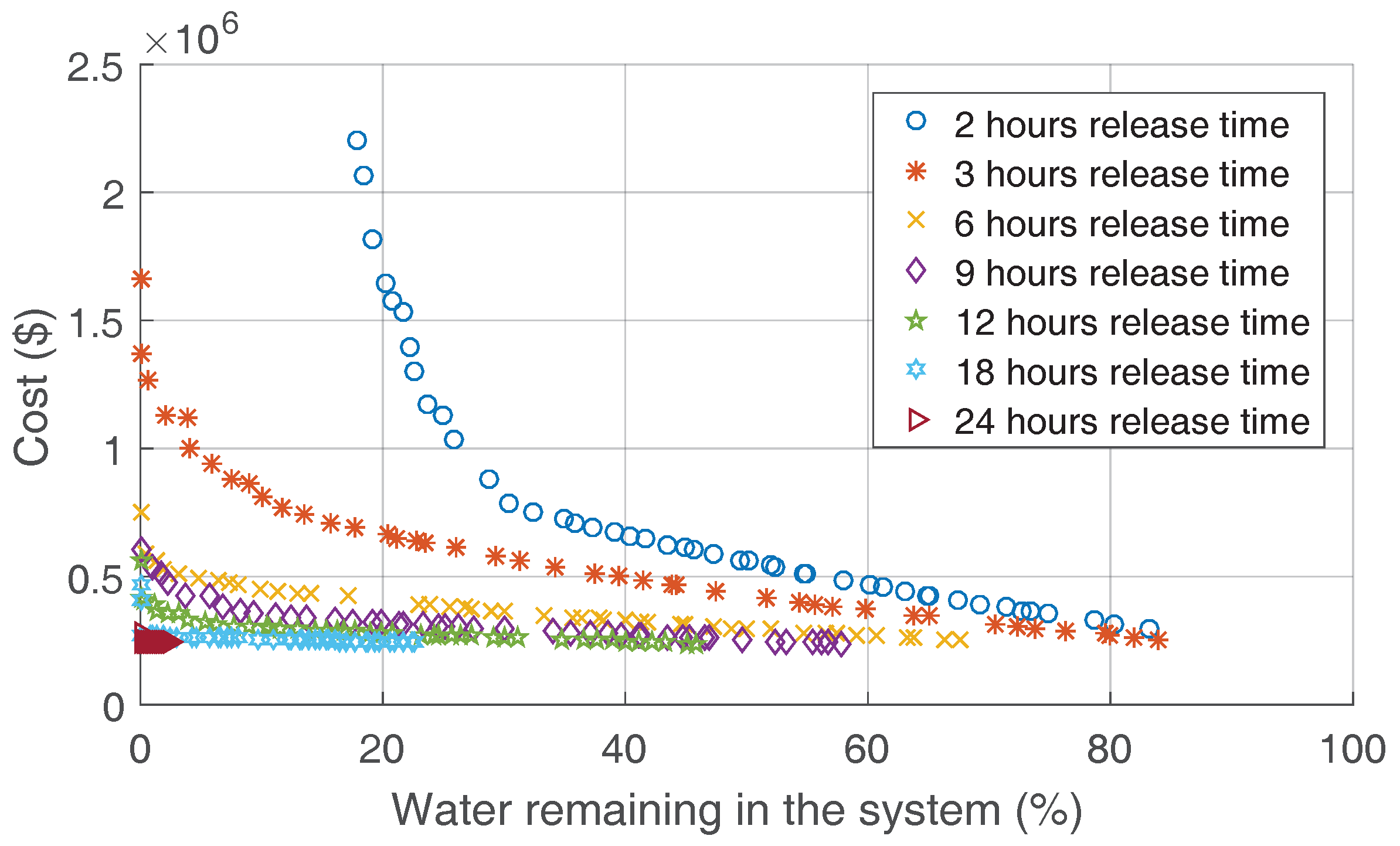
Pareto fronts for the two aforementioned objectives and seven releasing times are shown in Figure 12. A Pareto front (or Pareto frontier) is a set of nondominated optimal solutions where no objective can be improved without sacrificing at least one other objective (e.g., [40]). On the other hand, a solution is referred to as dominated by a second solution if, and only if, the second solution is equally good or better than the first solution with respect to all objectives (e.g., [40]). Each point on a Pareto front is associated with a cost and the percentage of water released from the wetlands. The latter is equal to 100% minus the percentage of water remaining in the wetlands. Since each point on the Pareto front is indifferent in the context of multi-objective optimization, selection of a point from the Pareto front merely depends on the preference of the decision maker. For example, for a releasing time of 3 h, the decision maker may choose a relatively low cost option ($250 K) with a relatively small percentage of water release (100% − 80% = 20%). Alternatively, a more balanced option would be that with a $450 K cost and 50% water release. A solution with $650 K cost and 80% water release (20% of water remaining in the system) would be a better choice for faster drainage of the wetlands. Furthermore, as can be observed in Figure 12 and as is expected, for the same cost, the larger the releasing time, the larger the percentage of water release. Likewise, for the same percentage of water release, the larger the releasing time, the smaller the cost.

A few solutions for the optimal number of $24{}^{″}$ pipes for each wetland for the 3-h releasing time are shown in Figure 13. Although all the scenarios in Figure 13 have the same releasing time of 3 h, each scenario has different results with respect to how much water is released in the 3 h. For example, the scenario depicted with diamond markers releases 99.99% of the water but with a larger cost (i.e., larger number of pipes). The scenario depicted with green five-pointed star (pentagram) markers markers releases 19.99% of the water at a smaller cost (smaller number of pipes). Furthermore, as can be observed in Figure 13 and as is expected, the most downstream wetlands have a larger number of pipes in comparison to the most upstream wetlands (see pipe network in Figure 4). To evaluate how the number of pipes changes with the pre-specified releasing time, Figure 14 compares the solutions of optimal pipe diameters for 80% water release and five different releasing times (2, 3, 6, 12, and 18 h). As it is expected, the larger the releasing time, the smaller the number of pipes required.

3. Benefit–Cost Analysis

The benefit–cost analysis was prepared using the best information the authors could find.

Table 2. Cumulative value of wetland services per acre for the Houston–Galveston area for the periods 2018–2037, 2018–2047, and 2018–2067 (Adapted from [41]).

Ecosystem Services	Unitary Value Ref: Houston-Wilderness	Value in 2018 per Acre	Cum. Value 2018–2037 per Acre	Cum. Value 2018–2047 per Acre	Cum. Value 2018–2067 per Acre
Water Supply (Nontidal)	$9320/acre/year Year 2010	$11,049	$272,508	$458,920	$974,779
Water Quality (Nontidal)	$3500/acre/year Year 2010	$4149	$102,337	$172,341	$366,065
Stormw. Regul./Flood Protect. (Nontidal)	$7990/acre/year Year 2010	$9472	$233,620	$393,430	$835,674
Climate Regul./Carbon Sequest. Palustrine Emergent (100%)	$100.4/acre/year Year 2010	$119	$2936	$4944	$10,501
Recreation	$2092/acre/year Year 2012	$2377	$58,620	$98,720	$209,689
Total		$27,166	$670,021	$1,128,355	$2,396,707

provides the cumulative value of wetland services per acre for the Houston–Galveston area for three periods (20, 30, and 50 years). The second column in Table 2 shows the value of wetland services for the Houston–Galveston area as reported by [41]. The third column of Table 2 presents the updated values of wetland services for 2018 U.S. dollars using an inflation rate of 2.15%, which was the average U.S. inflation rate between 1996 and 2016 (http://www.usinflationcalculator.com/). Columns 5–7 in Table 2 present the cumulative value of wetland services per acre assuming that the system enters in service in 2018 and the periods of service are 20, 30, and 50 years, respectively.

According to the compiled information by Houston–Wilderness ([41]), wetlands in the Houston–Galveston area provide the following benefits.

• Water supply (nontidal): $9320/acre/year ($2010). Benefit provided (nontidal): 100,000 gallons/ acre/day (wetlands can provide water at a lower cost than procuring it elsewhere).
• Water quality (nontidal): Median $3500/acre/year ($2010). Benefit provided (nontidal): Can filter 63% of nitrogen, 45% of phosphorous.
• Stormwater regulation/flood protection (nontidal): $7990/acre/year ($2010). Benefit provided (nontidal): Wetlands can typically store one million gallons of floodwater per acre.
• Climate regulation/carbon sequestration: $68–236/acre/year ($2010). Palustrine emergent (100%)—$100.4/acre/year. Because our proposed wetlands are relatively shallow, the wetlands would be mostly palustrine emergent. Benefit provided: Wetlands store between 75,000 and 260,000 lbs of carbon per acre.
• Recreation: $2092/acre/year ($2012). Benefit Provided: Birding/hunting.

Table 3. Construction and Maintenance Costs per acre for the Houston–Galveston area for the periods 2018–2037, 2018–2047, and 2018–2067.

Description	Unitary Value (See References in This Column)	Value per Acre Year 2018	Value at 2037 or Cum. Value 2018–2037 per Acre	Value at 2047 or Cum. Value 2018–2047 per Acre	Value at 2067 or Cum. Value 2018–2067 per Acre
Land costs	$50,000/acre (Year 2017) (Estimated)	$51,075	$76,513	$94,650	$144,840
Design and Engineering	$500,000 (entire system) (Year 2017) (Estimated)	$552	$827	$1023	$1566
Earthwork (cut)	$12/cu. yd. (Year 2017) (Aver. of 3 contractors in Houston-Galveston)	$6704	$10,043	$12,424	$19,012
Earthwork (fill)	$12/cu. yd. (Year 2017) (Aver. of 3 contractors in Houston-Galveston)	$6624	$9924	$12,276	$18,785
Drainage pipes and Automated gates	$650,000 (entire system) (Year 2017) (Optimiz. in this paper)	$718	$1075	$1330	$2036
Installing vegetation	$10000/acre (Year 2017) (Texas Coastal Watershed Program 2017)	$10,215	$15,303	$18,930	$28,968
Equipment for remote operation of gates	$11,000,000 (entire system) (Year 2017) (Omnisite)	$12,148	$18,198	$22,511	$34,448
Mainten. of remote operation of gates and cel. annual fees	$575,000/year (Year 2017) (Omnisite 2017)	$635	$951	$1177	$1801
Wetland maintenance (does not include Gate remote operat.)	9.1% of construction cost per year Weiss et al. (2005)	$2208	$54,452	$91,700	$194,776
Total		$90,879	$187,286	$256,021	$446,232

provides the costs of construction and maintenance of the UHCC wetland system. According to [42], the construction cost of wetlands (e.g., costs of earthwork and vegetation planting) ranges between 0.60 and 1.25 dollars per cubic feet of wetland, where 1997 is the base year for the cost data. Using the above data, for a 2.5-foot-deep wetland, the cost in 1997 dollars would range between about $65,000 and $136,000 per acre, which updated to 2018 dollars would range between $101,344 and $212,044. As shown in the third column of Table 3, the cost of our hypothetical wetland system in 2018 dollars would be $90,879 per acre. This amount is near the low end of the range obtained in [42]. The low cost is expected as the construction of the hypothetical wetland system would involve minimal excavation.

As discussed in the optimization section, the total cost of the drainage for the hypothetical wetland system for releasing 80% of the water in 3 h is $650,000, which gives an average of $703 per acre. This means that the drainage cost is much smaller compared to the construction cost of a wetland. The maintenance cost for constructed wetlands reported in the literature is highly variable. For instance the U.S. Environmental Protection Agency ([42]) considers an annual maintenance cost of 2% of the construction cost. The authors of [43] consider an annual maintenance cost between 4% and 14.2% of the construction cost. In this study, two maintenance costs are considered, one for the wetland including the drainage system and another for the equipment/software for the remote operation of gates (e.g., SCADA-type control) including the fees for cellular or satellite connection. For the wetland/drainage system, an annual maintenance cost of 9.1% of the construction cost is considered, which is the average of the percentage in [43]. For the gate remote operation equipment/software/connection fees, the spreadsheet in Omnisite (Omnisite [44]) was used. The vegetation costs were obtained with information in [45].

Table 4. Benefit/cost ratios for the Houston–Galveston area for the periods 2018–2037, 2018–2047, and 2018–2067.

Description	Total Value 2018–2037 (925 Acres)	Total Value 2018–2047 (925 Acres)	Total Value 2018–2067 (925 Acres)
Construction and maintenance costs	$173,239,346	$236,819,296	$412,764,576
Value of benefits of ecosystem services New flood control (FC) = 1 × FC with no storag. manag.	$619,769,648	$1,043,728,778	$2,216,954,114
Benefit/cost ratio	3.58	4.41	5.37
Value of benefits of ecosystem services New FC = 2 × FC with no storag. manag.	$835,868,379	$1,407,651,834	$2,989,952,553
Benefit/cost ratio	4.82	5.94	7.24
Value of benefits of ecosystem services New FC = 3 × FC with no storag. manag.	$1,051,967,110	$1,771,574,890	$3,762,950,991
Benefit/cost ratio	6.07	7.48	9.12

presents the comparison of construction/maintenance costs and the benefits provided by the wetlands for periods of 20, 30, and 50 years assuming that the flood control due to dynamic management of wetland storage is respectively one, two, and three times that with no management. As can be observed in Table 4, in general, the benefit value of wetland services far surpasses the costs of construction and maintenance of the UHCC wetland system for the three considered periods of analysis and for the three degrees of dynamic management of wetland storage. Furthermore, the benefit/cost ratios increase with the period of analysis.

In a similar way to Table 4,

Table 5. Benefit/cost ratios for the Houston–Galveston area for the periods 2018–2037, 2018–2047, and 2018–2067 assuming that flood protection is the only benefit provided by wetlands.

Description	Total Value 2018–2037 (925 Acres)	Total Value 2018–2047 (925 Acres)	Total Value 2018–2067 (925 Acres)
Construction and maintenance costs	173,239,346	236,819,296	412,764,576
Value of benefits (New flood control (FC) = 0 × FC with no storag. manag.)	216,098,731	363,923,056	772,998,439
Benefit/cost ratio	1.25	1.54	1.87
Value of benefits New FC = 0.5 × FC with no storag. manag.	324,148,096	545,884,584	1,159,497,658
Benefit/cost ratio	1.87	2.31	2.81
Value of benefits New FC = 1 × FC with no storag. manag.	432,197,462	727,846,112	1,545,996,878
Benefit/cost ratio	2.49	3.07	3.75
Value of benefits New FC = 2 × FC with no storag. manag.	648,296,193	1,091,769,168	2,318,995,316
Benefit/cost ratio	3.74	4.61	5.62
Value of benefits New FC = 4 × FC with no storag. manag.	1,080,493,655	1,819,615,280	3,864,992,194
Benefit/cost ratio	6.24	7.68	9.36

presents the benefit/cost ratios assuming that flood control is the only benefit provided by wetlands (e.g., not considering the value of other ecosystem services). As can be observed in Table 5, the benefit/cost ratio is larger than one even when the proposed water storage management does not provide any additional benefit to that with no management. Table 5 also shows that whenever flood control with no management is improved by 100%, the benefit/cost ratio, taking into account flood control only, would increase by 125%, 154%, and 187% for the 20-, 30-, and 50-year periods, respectively. In addition, Table 5 shows that the benefit/cost ratio, taking into account flood control only, would be at least 1.87 as long as the proposed dynamic management of wetland storage improves flood control by 50% compared to that with no management.

4. Conclusions

The work presented herein addresses part of a larger topic which is to dynamically manage the water storage of a system of interconnected wetlands for minimizing floods. The scope of this paper is limited to the benefit–cost analysis of dynamic management of storage for a system of wetlands for improving flood control. The key findings are as follows:

• In general, the benefit value of wetland services far surpasses the costs of construction and maintenance of the UHCC wetland system for the three considered periods of analysis and the three degrees of dynamic management of wetland storage.
• The benefit/cost ratios increase with the period of analysis.
• Considering flood protection only (e.g., not considering the value of other ecosystem services), as long as dynamic management of wetland storage increases flood protection by about 50% compared to that with no management, the construction of a wetland system would have a benefit/cost ratio of at least 1.9.

References

- Kusler, J. Multi-Objective Wetland Restoration in Watershed Contexts; Technical Report; Association of State Wetland Managers: Berne, NY, USA, 2004. [Google Scholar]
- Flotemersch, J.E.; Leibowitz, S.G.; Hill, R.A.; Stoddard, J.L.; Thoms, M.C.; Tharme, R.E. A Watershed Integrity Definition and Assessment Approach to Support Strategic Management of Watersheds. River Res. Appl. 2016, 32, 1654–1671. [Google Scholar] [CrossRef]
- Chescheir, G.M.; Gilliam, J.W.; Skaggs, R.W.; Broadhead, R.G. Nutrient and sediment removal in forested wetlands receiving pumped agricultural drainage water. Wetlands 1991, 11, 87–103. [Google Scholar] [CrossRef]
- Bullock, A.; Acreman, M. The role of wetlands in the hydrological cycle. Hydrol. Earth Syst. Sci. 2003, 7, 358–389. [Google Scholar] [CrossRef]
- Timoney, K. Factors influencing wetland plant communities during a flood-drawdown cycle in the Peace-Athabasca Delta, Northern Alberta, Canada. Wetlands 2008, 28, 450–463. [Google Scholar] [CrossRef]
- Lee, S.Y.; Hamlet, A.F.; Fitzgerald, C.J.; Burges, S.J. Optimized Flood Control in the Columbia River Basin for a Global Warming Scenario. J. Water Resour. Plan. Manag. 2009, 135, 440–450. [Google Scholar] [CrossRef]
- Acreman, M.; Holden, J. How Wetlands Affect Floods. Wetlands 2013, 33, 773–786. [Google Scholar] [CrossRef]
- De Wilde, M.; Puijalon, S.; Vallier, F.; Bornette, G. Physico-Chemical Consequences of Water-Level Decreases in Wetlands. Wetlands 2015, 35, 683–694. [Google Scholar] [CrossRef]
- Mitsch, W.J.; Bernal, B.; Hernandez, M.E. Ecosystem services of wetlands. Int. J. Biodivers. Sci. Ecosyst. Serv. Manag. 2015, 11, 1–4. [Google Scholar] [CrossRef]
- Sterzyńska, M.; Pižl, V.; Tajovský, K.; Stelmaszczyk, M.; Okruszko, T. Soil Fauna of Peat-Forming Wetlands in a Natural River Floodplain. Wetlands 2015, 35, 815–829. [Google Scholar] [CrossRef]
- Kadlec, R.H. Large Constructed Wetlands for Phosphorus Control: A Review. Water 2016, 8, 243. [Google Scholar] [CrossRef]
- Skagen, S.K.; Burris, L.E.; Granfors, D.A. Sediment Accumulation in Prairie Wetlands under a Changing Climate: the Relative Roles of Landscape and Precipitation. Wetlands 2016, 36, 383–395. [Google Scholar] [CrossRef]
- Lee, L.H. Perspectives on Landscape Aesthetics for the Ecological Conservation of Wetlands. Wetlands 2017, 37, 381–389. [Google Scholar] [CrossRef]
- Miller, J.O.; Ducey, T.F.; Brigman, P.W.; Ogg, C.O.; Hunt, P.G. Greenhouse Gas Emissions and Denitrification within Depressional Wetlands of the Southeastern US Coastal Plain in an Agricultural Landscape. Wetlands 2017, 37, 33–43. [Google Scholar] [CrossRef]
- Interagency Floodplain Management Review Committee. Sharing the Challenge: Floodplain Management into the 21st Century: Report of the Interagency Floodplain Management Review Committee to the Administration Floodplain Management Task Force; Executive Office of the President: Washington, DC, USA, 1994.
- McCuskey, S.A.; Conger, A.W.; Hillestad, H.O. Design and implementation of functional wetland mitigation: Case studies in Ohio and South Carolina. Water Air Soil Pollut. 1994, 77, 513–532. [Google Scholar] [CrossRef]
- United States Environmental Protection Agency (USEPA). Design Manual, Constructed Wetlands and Aquatic Plant Systems for Municipal Water Treament; Report EPA/625/1-88/022; U.S. Environmental Protection Agency: Washington, DC, USA, 1998.
- United States Environmental Protection Agency (USEPA). General Considerations. In A Handbook of Constructed Wetlands, A Guide to Creating Wetlands for Agricultural Wastewater, Domestic Wastewater, Coal Mine Drainage, Stormwater in the Mid-Atlantic Region; Technical Report; U.S. Environmental Protection Agency: Washington, DC, USA, 2000; Volume 1. [Google Scholar]
- Wooster, R.A.; Reddick, D.C.; McNamee, G.L. Texas. 2018. Available online: https://www.britannica.com/place/Texas-state (accessed on 1 March 2018).
- Glennie, C.L.; Carter, W.E.; Shrestha, R.L.; Dietrich, W.E. Geodetic imaging with airborne LiDAR: the Earth’s surface revealed. Rep. Prog. Phys. 2013, 76, 086801. [Google Scholar] [CrossRef] [PubMed]
- Steele, M.K.; Heffernan, J.B.; Bettez, N.; Cavender-Bares, J.; Groffman, P.M.; Grove, J.M.; Hall, S.; Hobbie, S.E.; Larson, K.; Morse, J.L.; et al. Convergent Surface Water Distributions in U.S. Cities. Ecosystems 2014, 17, 685–697. [Google Scholar] [CrossRef] [Green Version]
- Palta, M.M.; Grimm, N.B.; Groffman, P.M. “Accidental” urban wetlands: ecosystem functions in unexpected places. Front. Ecol. Environ. 2017, 15, 248–256. [Google Scholar] [CrossRef]
- Donohue, I.; Hillebrand, H.; Montoya, J.M.; Petchey, O.L.; Pimm, S.L.; Fowler, M.S.; Healy, K.; Jackson, A.L.; Lurgi, M.; McClean, D.; et al. Navigating the complexity of ecological stability. Ecol. Lett. 2016, 19, 1172–1185. [Google Scholar] [CrossRef] [PubMed]
- Sharitz, R.R.; Batzer, D.P.; Pennings, S.C. Ecology of freshwater and estuarine wetlands: An introduction. In Ecology of Freshwater and Estuarine Wetlands, 2nd ed.; Batzer, D.P., Sharitz, R.R., Eds.; University of California Press: Oakland, CA, USA, 2014. [Google Scholar]
- McPeek, M.A. Trade-Offs, Food Web Structure, and the Coexistence of Habitat Specialists and Generalists. Am. Nat. 1996, 148, S124–S138. [Google Scholar] [CrossRef]
- McPeek, M.A. The Consequences of Changing the Top Predator in a Food Web: A Comparative Experimental Approach. Ecol. Monogr. 1998, 68, 1–23. [Google Scholar] [CrossRef]
- Snodgrass, J.W.; Komoroski, M.J.; Bryan, A.L.; Burger, J. Relationships among Isolated Wetland Size, Hydroperiod, and Amphibian Species Richness: Implications for Wetland Regulations. Conserv. Biol. 2000, 14, 414–419. [Google Scholar] [CrossRef]
- Ehrenfeld, J.G. The expression of multiple functions in urban forested wetlands. Wetlands 2004, 24, 719–733. [Google Scholar] [CrossRef]
- Tarr, T.L.; Baber, M.J.; Babbitt, K.J. Macroinvertebrate community structure across a wetland hydroperiod gradient in southern New Hampshire, USA. Wetl. Ecol. Manag. 2005, 13, 321–334. [Google Scholar] [CrossRef]
- Brooks, R.T. Annual and seasonal variation and the effects of hydroperiod on benthic macroinvertebrates of seasonal forest (“vernal”) ponds in central Massachusetts, USA. Wetlands 2000, 20, 707–715. [Google Scholar] [CrossRef]
- Batzer, D.P.; Resh, V.H. Wetland management strategies that enhance waterfowl habitats can also control mosquitoes. Am. Mosq. Control Assoc. 1992, 8, 117–125. [Google Scholar]
- Batzer, D.P.; Wissinger, S.A. Ecology of insect communities in nontidal wetlands. Annu. Rev. Entomol. 1996, 41, 75–100. [Google Scholar] [CrossRef] [PubMed]
- Moulton, D.W.; Jacob, J. Texas Coastal Wetlands Guidebook; Publication TAMU-SG-00-605 (r); Texas Sea Grant: College Station, TX, USA, 2000. [Google Scholar]
- Tiner, R. Geographically isolated wetlands of the United States. Wetlands 2003, 23, 494–516. [Google Scholar] [CrossRef]
- Jacob, J.; Pandian, K.; Lopez, R.; Briggs, H. Houston-Area Freshwater Wetland Loss, 1992–2010; Erpt-002, Tamu-sg-14-303; Texas A&M Agrilife Extension: College Station, TX, USA, 2014.
- Wilcox, B.P.; Dean, D.D.; Jacob, J.S.; Sipocz, A. Evidence of Surface Connectivity for Texas Gulf Coast Depressional Wetlands. Wetlands 2011, 31, 451–458. [Google Scholar] [CrossRef]
- Leon, A.S.; Alnahit, A. A Remotely Controlled Siphon System for Dynamic Water Storage Management. In Proceedings of the 6th IAHR International Symposium on Hydraulic Structures, Portland, OR, USA, 27–30 June 2016; pp. 1–11. [Google Scholar]
- Leon, A.S.; Chen, D.; Yolcu, A. Optimal drainage of interconnected wetlands for flood control. Appl. Water Eng. Res. Under review 2017. [Google Scholar]
- Deb, K.; Pratap, A.; Agarwal, S.; Meyarivan, T. A fast and elitist multiobjective genetic algorithm: NSGA-II. IEEE Trans. Evolut. Comput. 2002, 6, 182–197. [Google Scholar] [CrossRef]
- Chen, D.; Leon, A.S.; Gibson, N.L.; Hosseini, P. Dimension reduction of decision variables for multireservoir operation: A spectral optimization model. Water Resour. Res. 2016, 52, 36–51. [Google Scholar] [CrossRef]
- Houston-Wilderness. Ecosystem Services. 2017. Available online: http://houstonwilderness.org/ecosystem-services/ (accessed on 5 July 2017).
- United States Environmental Protection Agency (USEPA). Preliminary Data Summary of Urban Storm Water Best Management Practices; Report EPA-821-R-99-012; U.S. Environmental Protection Agency: Washington, DC, USA, 1999.
- Weiss, P.T.; Gulliver, J.S.; Erickson, A.J. The Cost and Effectiveness of Stormwater Management Practices; Report 2005-23; Minnesota Department of Transportation: Saint Paul, MN, USA, 2005.
- Omnisite. OmniSite Vs. SCADA. 2016. Available online: http://www.omnisite.com/ (accessed on 5 July 2017).
- Texas Coastal Watershed Program. Cost and Maintenance. 2017. Available online: http://tcwp.tamu.edu/stormwater/wetlands/cost-and-maintenance/ (accessed on 5 July 2017).
Figure 1.
Google Earth view of the University of Houston Coastal Center (UHCC), southeast of Houston, Texas, United States.
Figure 2.
Plan view of the UHCC wetland system before (left) and after being virtually modified (right).
Figure 3.
A three-dimensional (3D) sketch of the UHCC wetland system after being virtually modified.
Figure 4.
Layout of drainage. Note that wetland 1 (W1) receives the water from wetlands 2 (W2) to 4 (W4). Then the combined water is discharged to the existing lateral ditch at a single discharge point.
Figure 5.
Plan view of the four wetland system displaying the 14 one-acre terrestrial islands intended as an ecological habitat. This plan view does not show the drainage system.
Figure 6.
Cross-sectional view A-A. This section shows the intake for the “flood” pipe.
Figure 7.
Cross-sectional view B-B. This section shows the intake for the “overflow” pipe.
Figure 8.
Cross-sectional view C-C. This section shows the intake for the “flood” and “overflow” pipes.
Figure 9.
Cross-sectional view D-D. This section shows the side view of the one-acre terrestrial island.
Figure 10.
Cross-sectional view E-E. This section shows the side view of flow discharge from the downstream wetland to the drainage ditch.
Figure 11.
Percentage of water released from the wetlands versus time step.
Figure 12.
Optimal trade-off between percentage of water remaining in the wetland system and piping/automated valve cost.
Figure 13.
Optimal pipe diameters for a 3-h releasing time.
Figure 14.
Optimal pipe diameters for releasing 80% of the water under different releasing times.