High-Frequency Monitoring of Suspended Sediment Variations for Water Quality Evaluation at Deep Bay, Pearl River Estuary, China: Influence Factors and Implications for Sampling Strategy

Abstract

Suspended sediment (SS) is an important water quality indicator of coastal and estuarine ecosystems. Field measurement and satellite remote sensing are the most common approaches for water quality monitoring. However, the efficiency and precision of both methods are typically affected by their sampling strategy (time and interval), especially in highly dynamic coastal and estuarine waters, because only limited measurements are available to analyze the short-term variations or the long-term trends of SS. Dramatic variations of SS were observed, with standard deviation coefficients of 48.9% and 54.1%, at two fixed stations in Deep Bay, China. Therefore, it is crucial to resolve the temporal variations of SS and its main influencing factors, and thus to develop an improved sampling strategy for estuarine ecosystems. Based on two years of continuous high-frequency measurements of SS and concurrent tidal and meteorological data, we demonstrated that the tide is the dominant factor influencing the SS variation among tide, wind (speed and direction), and rainfall in Deep Bay, China. For the monitoring of maximum suspended sediment concentration (SSC), the recommended optimum sampling time coincides with the occurrence of the ebb tides, whereas multiple sampling times are recommended for monitoring of minimum SSC. Although variations of SS are also affected by other factors, the recommended sampling strategy could capture the maximum and minimum SSC variations exactly more than 85% days in a year on average in Deep Bay. This study provides a baseline of SS variation and direct sampling strategy guidance for future SS monitoring and could be extended to other coastal or estuarine waters with similar climatological/tidal exposures.

1. Introduction

Coastal and estuarine waters are some of the most important ecosystems as they have a direct connection with human society, and provide value for recreation, food supply, commerce, transportation, and human health [1]. Since coastal and estuarine waters are particularly vulnerable to human activities and climate changes [2,3,4,5], effective monitoring methods are required to improve the management and protection of these regions. Suspended sediment (SS) is one of the most important parameters of water quality of estuarine waters, which are often optically complex [6,7]. Moreover, SS is the carrier of various nutrients and pollutants in water, altering the water transparency and thereby affecting the amount of incident radiation at different water depths, thus impacting the environment for aquatic organisms [8]. In addition, sediment dynamics have considerable impacts in terms of geomorphology, geochemical cycles [9], biogeochemistry [10], microbiology [11], benthic environment, coral reefs, and seagrass communities [12]. It is, therefore, of great importance to continue to improve monitoring of SS.

SS is influenced by natural (e.g., climatological and tidal) and human factors and varies substantially among different environments. Some studies have suggested that the resuspension and transportation of SS are combined effects of natural factors, such as wind, rainfall, flood fronts, waves, tidal currents, precipitation, and discharge under different conditions [13,14,15,16,17,18,19,20,21]. Wind is one of the dominant factor influencing SS in the Mekong River delta coast during monsoon periods [19]. Furthermore, rainfall was identified as one of the dominant factors in controlling suspended sediment concentration (SSC) in the Araguás Catchment, Spain based on classical statistical techniques [22]. The magnitude of the tide was found to be of low importance in controlling SS on inner-shelf coral reefs in Townsville, Australia, based on continuous measurements of SSC, wind, current and wave data over a period of 4 months [20]. In addition, the sediment fluxes are also affected by human impacts such as land disturbance, reservoir construction, mining activity, soil and water conservation measures, and sediment control programs [23,24,25].

In many cases, the range in observed SS is very large; maximum SSC ranges between 11 and 8816 mg/L in Aixola, 35 to 1614 mg/L in Barrendiola, and 17 to 1595 mg/L in Añarbe, Spain after flood events [21]. In addition, the SS in coastal waters change considerably over time. The SS of coastal area yield relatively high values (>20 mg/L) and extremely high values (>200 mg/L) in winter because of the strong northwest monsoon [26]. Moreover, the SS is so dynamic that it shows a notable decrease over time at low tide and increases again 2–3 h after low tide for the transition of flood tide to ebb tide [27]. Furthermore, in the study of Yang et al. [28], the SS increased from hundreds to thousands of mg/L in Hangzhou Bay over only 24 h under the influence of tidal currents, and similar impacts of tide on the SS variations were also observed in Deep bay using time series remote sensing data [29]. In general, the main factor controlling the SS varies between environments and the SS varies considerably over a short time, which makes it difficult to monitor the SS.

For decades, monitoring of water quality changes has mainly depended upon in situ sampling and land-based or shipboard laboratory analysis, which is high-precision but costly and time- and labor-intensive [30]. Moreover, traditional field sampling methods are often limited in terms of spatial and temporal coverage to build a robust model, or to derive statistically meaningful results [31,32]. Remote sensing is superior to conventional methods for water resource monitoring because of its wider spatial coverage, stable long-term acquisition, and low cost [33,34]. Significant progress has been made in studying coastal and inland waters using remote sensing [1,35,36]. The application of remote sensing provides an effective solution for monitoring of the spatial distribution of SS and dynamic changes in SS over time, for example, MODIS and GOCI data are used to estimate total suspended matter concentration in coastal zones [28,37]. However, the sampling strategy (time and interval) is one of the major factors that influence the efficiency and precision of both in situ and remote sensing methods because, in most cases, only limited measurements (i.e., once a day for in situ or twice a day for remote sensing such as Terra/Aqua MODIS) are available to analyze the variations or the long-term trend of SS. This is particularly the case for regions with significant diurnal or semidiurnal variations in SS movements and for satellite observations with cloud contamination, bad weather conditions or sun glints [38,39,40].

High-frequency measurement is beneficial for monitoring highly dynamic SS and an inappropriate sampling strategy would lead to large biases. However, little research has focused on this topic. It has been shown that an inappropriate sampling strategy would cause a statistical error of more than 50% for water quality monitoring [41,42], and insufficient sampling frequency would introduce about 90% uncertainty for long-term trend analysis of water quality [40]. Consequently, there is an urgent need to understand the short-term variability and dominant factors controlling SS, and thus provide guidance for sampling strategy of SS. Studies on this topic will provide a baseline for further investigations of water quality [42]. In addition, the ongoing satellite ocean color missions call for thorough consideration of the trade-offs between requirements of water resource monitoring and instrument design, including the time and frequency for water quality observation.

This study aimed to resolve the main factors affecting SS in an estuarine environment and provide a baseline for sampling strategy. To achieve this, we applied a two-year high-frequency in situ measurement dataset of SS collected in Deep Bay, China. The following approach was taken to this study: (1) the short-term dynamics and temporal variations of SS was analyzed, (2) the factors affecting SS were then explored with concurrent tidal and meteorological data, (3) the dominant factor was determined and the influence on sampling strategy was examined, and (4) recommendations were made for SS sampling method.

2. Materials and Method

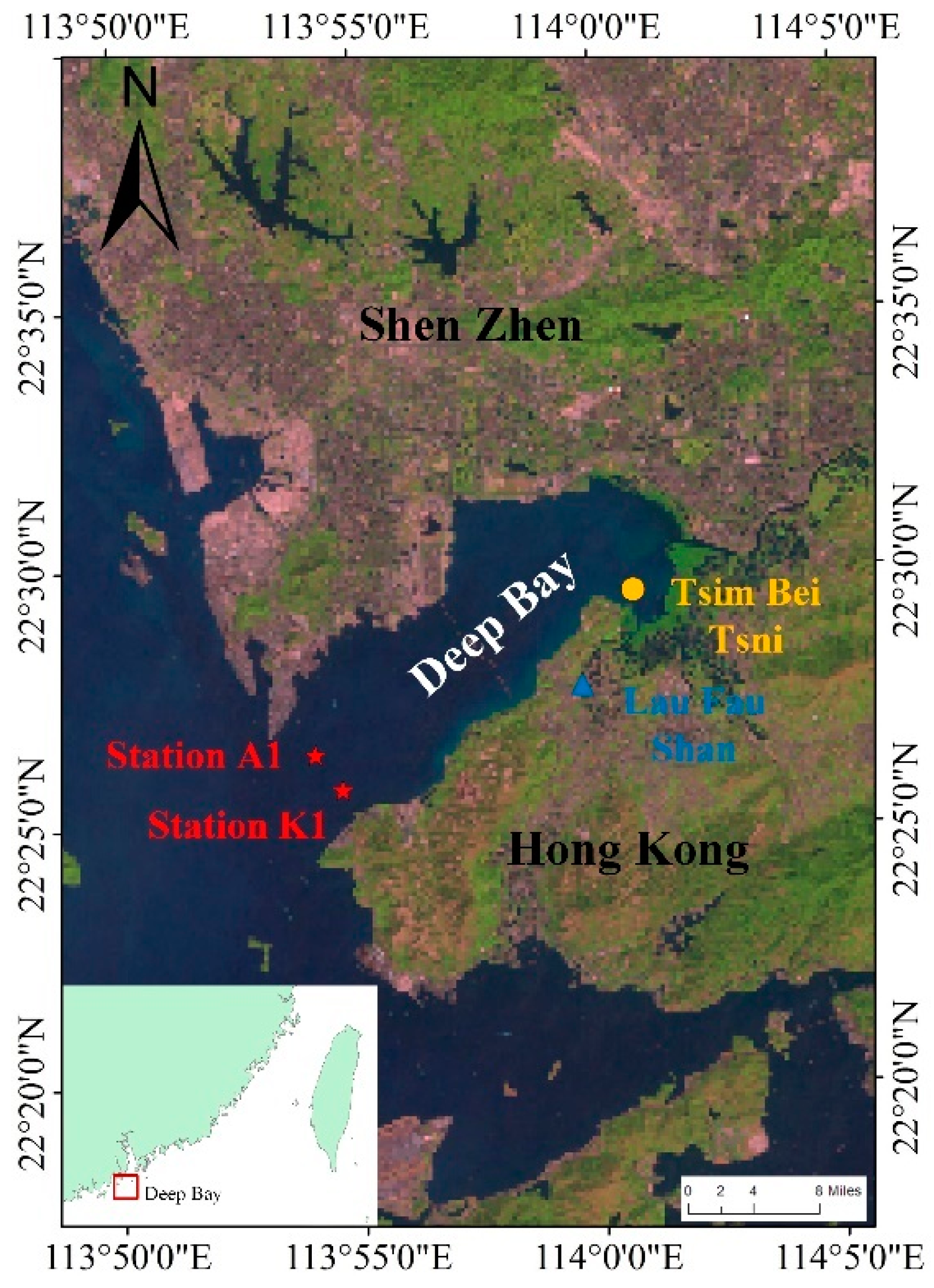
2.1. Study Area

Deep Bay (22°24′18″ N–22°32′12″ N, 113°53′06″ E–114°02′30″ E) is situated on the east shore of the Pearl River Estuary, between Shenzhen to the north, which is a special economic zone of China, and the New Territories of Hong Kong to the south (Figure 1). It is a shallow, semi-enclosed bay with an average water depth of about 3 m and a tidal range of about 1.4 m. It stretches about 17.5 km in the southwest–northeast direction, and from 4 to 10 km in the northwest–southeast direction [43]. Deep Bay is influenced by subtropical monsoon climate with abundant rainfall (average annual rainfall of 1926.4 mm). The monsoon season is from April to September, accounting for about 85% of annual rainfall. The average annual rainfall decreases from the southeast to the northwest of the region.

With the rapid development of cities around Deep Bay, the water quality has decreased considerably compared with nearby regions, especially the waters of Hong Kong (Environmental Protection Department (EPD), Marine Water Quality in Hong Kong in 2006), which has led to a great threat to the natural ecosystem and to oyster culturing [44,45]. The siltation in Deep Bay has been aggravated in recent years, the estuary elevation has risen, and land use change has resulted in a narrowing of the width of the mouth of the Shenzhen River. These factors exacerbated the Shenzhen River flood detention phenomenon, reducing the original flood control capacity. Moreover, Shenzhen River original sand discharge capacity has also been affected, causing serious siltation. Therefore, dramatic changes have occurred in SS of Deep Bay. Ref. [43] showed that the average sedimentation flux was 0.28 $\mathrm{g}·{\mathrm{cm}}^{-2}·{\mathrm{a}}^{-1}$, with an apparent sedimentation rate of 0.69 $\mathrm{cm}·{\mathrm{a}}^{-1}$ at a station in Deep Bay. Abrupt changes in rate and pattern of sedimentation have been identified and the strong monsoon might lead to the large sediment supplies in the Pearl River Mouth Basin [46]. Moreover, the tidal cycle has been identified as one of the major factors inducing the temporal and spatial variation of SSC [47].

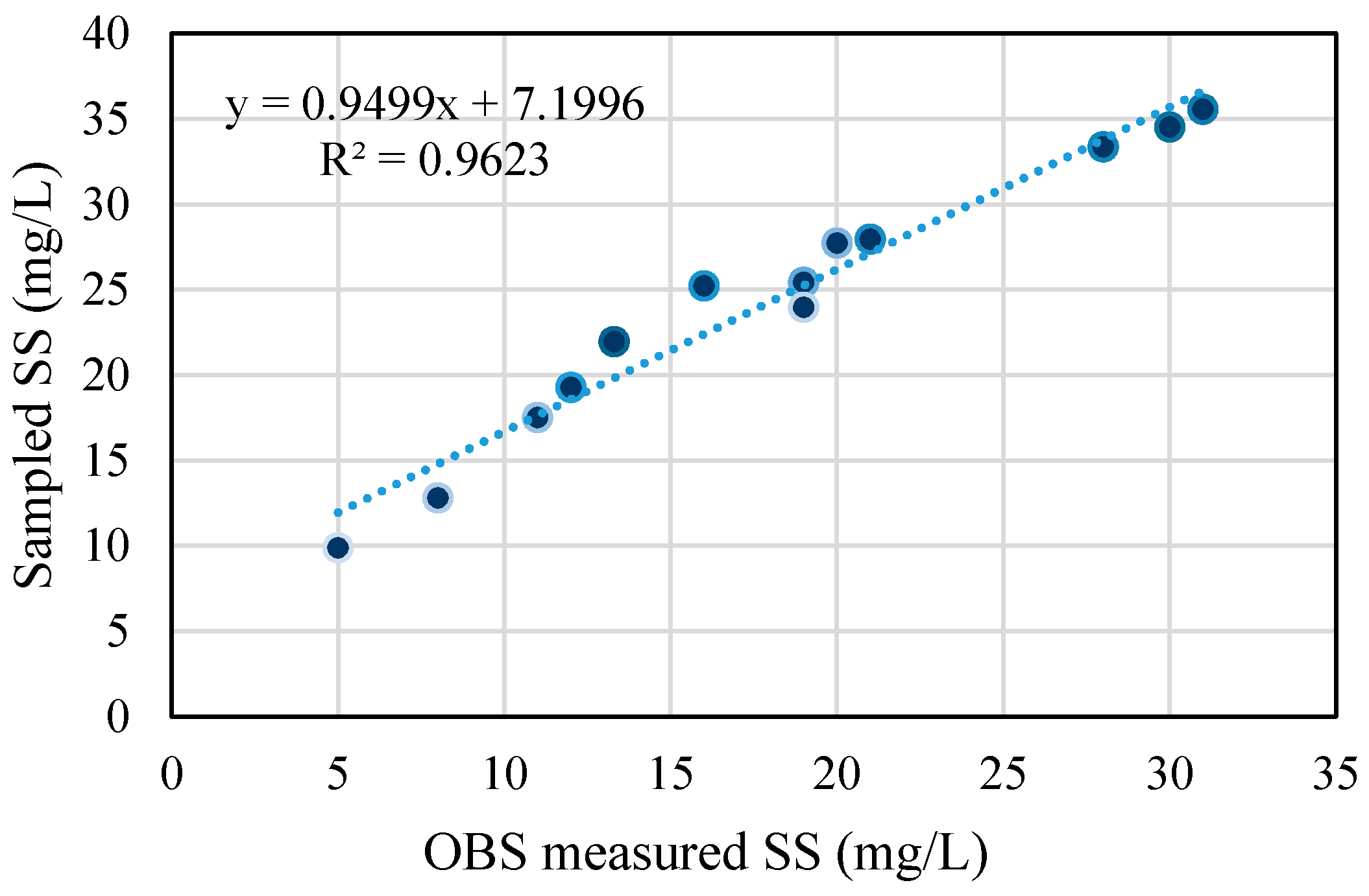
2.2. In-Situ Data Measurement

2.2.1. High Frequency SS Samples

The SS measurements were conducted at two fixed stations in Deep Bay (A1 to the north and K1 to the south; Figure 1). The two stations are located at the intersection of Deep Bay and the Pearl River, with an average local water depth of about 3 m and the sensor is positioned at depth of about 0.8 m below the water surface.

A backward light scattering sensor (OBS, the D & A Instrument Company in Logan, UT, USA, https://www.campbellsci.com/obs-3a) was used for SS measurement. The OBS measures the suspended particles by receiving the amount of infrared radiation and establishes the correlation between the water turbidity and the measured SS [48]. At constant diameter and low SSC (<5000 mg/L mud or <50,000 mg/L sand), the area of the illuminated particles is proportional to SS and OBS measurements provide accurate and reliable estimates of SS [49].

The range of the OBS measurement is 0–5000 mg/L. Furthermore, water samples at the depth of the OBS instrument were collected and returned to the laboratory for cross calibration and validation of the OBS measurements. The samples were analyzed using the drying method and weighed with an electronic balance with a precision of 0.1 μg to obtain a precise SSC. Three basic principles were followed for indoor cross calibration:

(1) The raw water sample of each instrument must be the water sample taken on the vertical line of the instrument.

(2) Calibration data consisted of at least 10 samples and should cover the dynamic range of sediment concentration.

(3) All field measurements must fall in the calibration curve and outliers were omitted. Two criterions were followed to detect and remove outliers: (1) all in situ measurements should be within the range of OBS (0–5000 mg/L) to make the calibration reliable; (2) the relative errors of SS between the OBS-measured and calculated from calibration curve were confined within 10%.

Calibration of the OBS was conducted using simultaneously collected field water samples every 7–10 days. During each calibration, at least 10 matchups of OBS and laboratory-analyzed SS were collected for cross calibration. The results of regression analysis on the calibration between OBS-measured turbidity and laboratory-analyzed SS on 2 March 2007 is shown in Figure 2, with a coefficient of determination ($R^2$) of 0.96, and a mean relative error of 6.45%. Long-term series-calibrated OBS measurements were also carried out at two stationary stations (A1 and K1 in Figure 1) in 2007 and 2008 and these were treated as the “ground truth” for continuous calibration of OBS data. More details on the collection of SS can be found in [50].

The OBS instrument was operated in an unattended manner and maintained every 7–10 days. The sampling interval was set as 30 min. During the operation period from January 2007 to December 2008, a total of 35,088 samples (all the samples were within the range of OBS) were collected for stations A1 and K1 (Figure 3A). These continuous and high-frequency SS measurements provide the first basic data for examination of temporal variation and development of an appropriate sampling strategy.

2.2.2. Tidal Data

Deep Bay is influenced by a semidiurnal tidal cycle, with two nearly equal high tides and two ebb tides every lunar day (about 24 h 50 min). The tidal data measured at Tsim Bei Tsui (TBT) (Figure 1) were provided by the Marine Department of Hong Kong. Tide samples were collected from 2007 to 2008, with the same frequency as the SS data (Figure 3B). The tidal range of Deep Bay is between −10 cm and 366 cm. Figure 4 presents long-term tide height for 2007 and 2008, and detailed tide heights of January 2008 and indicates that the tides are cyclical.

2.2.3. Meteorological Data

High-frequency meteorological data with the same sample interval as SS and tidal data were obtained at the Lau Fau Shan (LFS) meteorological station, including prevailing wind direction, wind speed and rainfall (Figure 3C,D).

The rainfall data were collected at the same time as the wind data. From May to August, the rainfall was heavier than that in other months, especially in June. The monthly mean rainfall and its standard deviation (STD) in 2007 and 2008 (Figure 5) show that the rain varied considerably in summer. In spring, there was nearly no rain.

Compared with rainfall, the wind speed was relatively stable in each month. The monthly mean wind speed was around 3.4 m/s. The mean and STD of wind speed are shown in Figure 6. The wind STDs ranged between 1 and 2.5 m/s. On the whole, the monthly wind was roughly consistent. However, during the summer, there was higher variation in the wind speed than in other seasons.

2.3. Analysis Method

2.3.1. Quantifying Spatial-Temporal Correlation Patterns of SS and Affecting Factors

To obtain an index that is not influenced by the absolute values of SS and affecting factors (tide, wind, and rainfall), all measures were normalized according to:

$$P_n\left(i,j\right)=\frac{P\left(i,j\right)}{MAX\left(P\right)}$$

(1)

where $P_n\left(i,j\right)$ and $P\left(i,j\right)$ refer to the $j_{\mathrm{th}}$ normalized and measured value of day $i$, respectively. $MAX\left(P\right)$ is the maximum value of all observations, and missing data were filled with 0.

The normalized SS, tide, wind speed, and rainfall data were arranged in columns representing 731 days (365 days in 2007 and 366 days in 2008), and rows denoting 24 h in a day. The data were then arranged and rasterized to form images, aiming to reveal the relationships between temporal variations of SS and tide, wind speed and rainfall. Furthermore, the main factors that influence the SS can also be determined intuitively using this approach.

Cross-correlation analysis was then applied to the SS and the main factors. Cross-correlation is a measure of similarity of two sets of time-series data as a function of the time lag between the two. For continuous measurements $f$ (SS) and $g$ (affecting factors), the cross-correlation is defined as [51,52]:

$$\left(f\ast g\right)\left(\tau \right)=\underset{-\infty }{\overset{\infty }{{\displaystyle \int }}}{f}^{\ast }\left(t\right)g\left(t+\tau \right)dt$$

(2)

where $f^{\ast }$ denotes the complex conjugate of $f$, and $\tau$ is the displacement, also known as time lag. A positive value of $\tau$ means that $g\left(t+\tau \right)$ occurs ahead of $g\left(t\right)$. Thus, cross-correlation can be used to determine the relationships among SS and affecting factors.

2.3.2. Statistical Indicators Analysis of SS and Affecting Factors

To determine an appropriate time to monitor the SS in Deep Bay, we analyzed the how the SS was affected by rainfall, wind speed and tides. Firstly, this study determines the time when the maximum and minimum SSC at station A1 and station K1 appear every day. Next, the time of the tide high water (THW) and time of tide low water (TLW) of the tide appear was determined with the same approach. The time interval between the maximum SSC and THW, the maximum SSC and TLW, the minimum SSC and THW, the minimum SSC and TLW were then calculated. Finally, 731 results for each of the four conditions were obtained and the histogram of time interval was produced.

Initially, the time interval was calculated by:

$$\Delta T=Time(A\left(TSS\left(i\right)\right)-Time\left(TID{E}_B\left(i\right)\right)$$

(3)

where $A$ is the maximum or minimum function, $B$ is the THW or TLW and $i$ is day $i$.

Then, we counted the time intervals in (5), and fitted the results according to (6) which is in accordance with Gaussian distribution to determine whether the results are reliable.

$$\mathrm{X}\left(i\right)={\displaystyle \sum }\left(\Delta T=i\right)$$

(4)

$$\mathrm{y}=y_0+A{e}^{-\frac{{\left(X-X_c\right)}^2}{2w^2}}$$

(5)

where $y_0$, $A$, $w$ and $X_c$ are the fit parameters.

3. Results

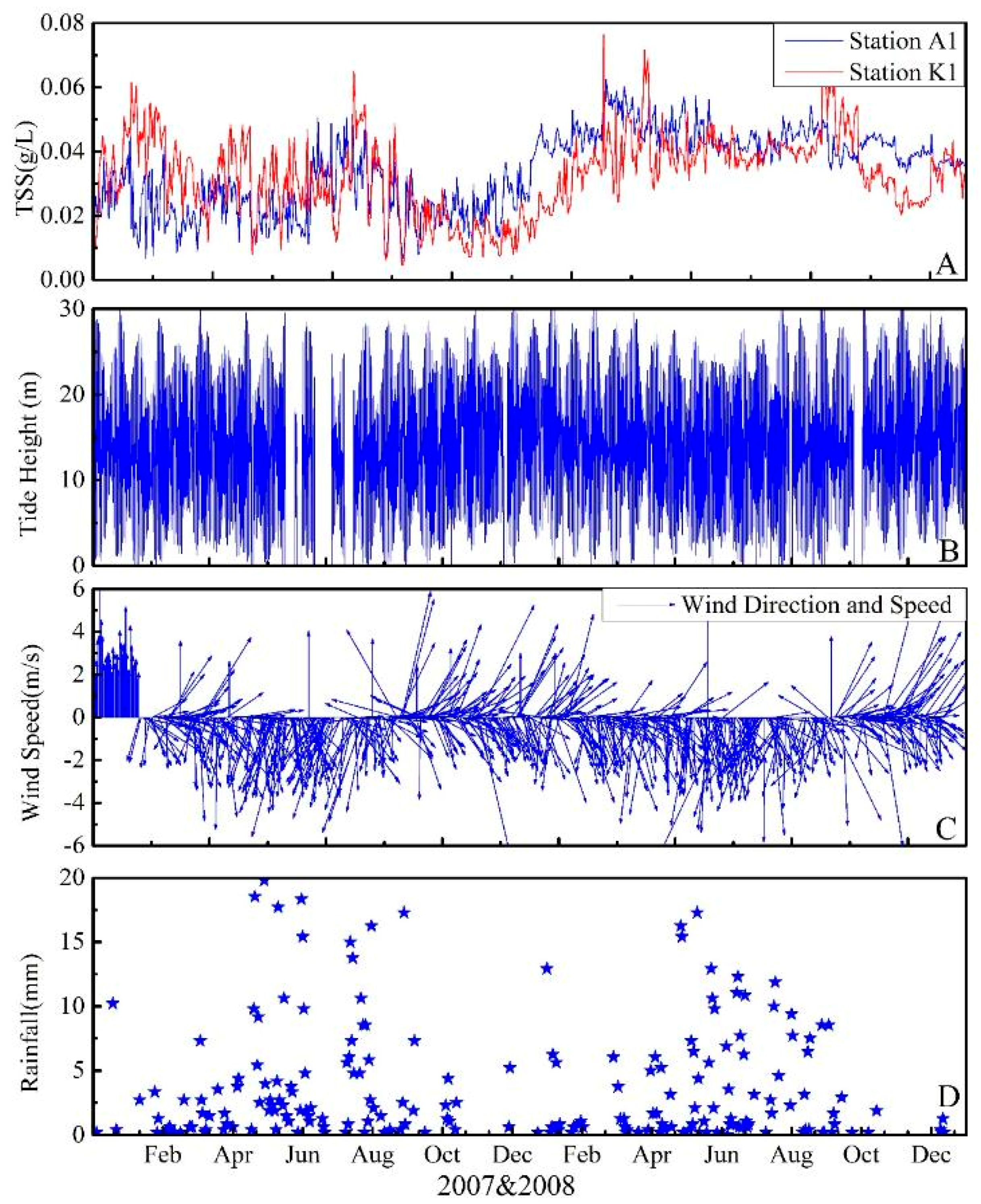
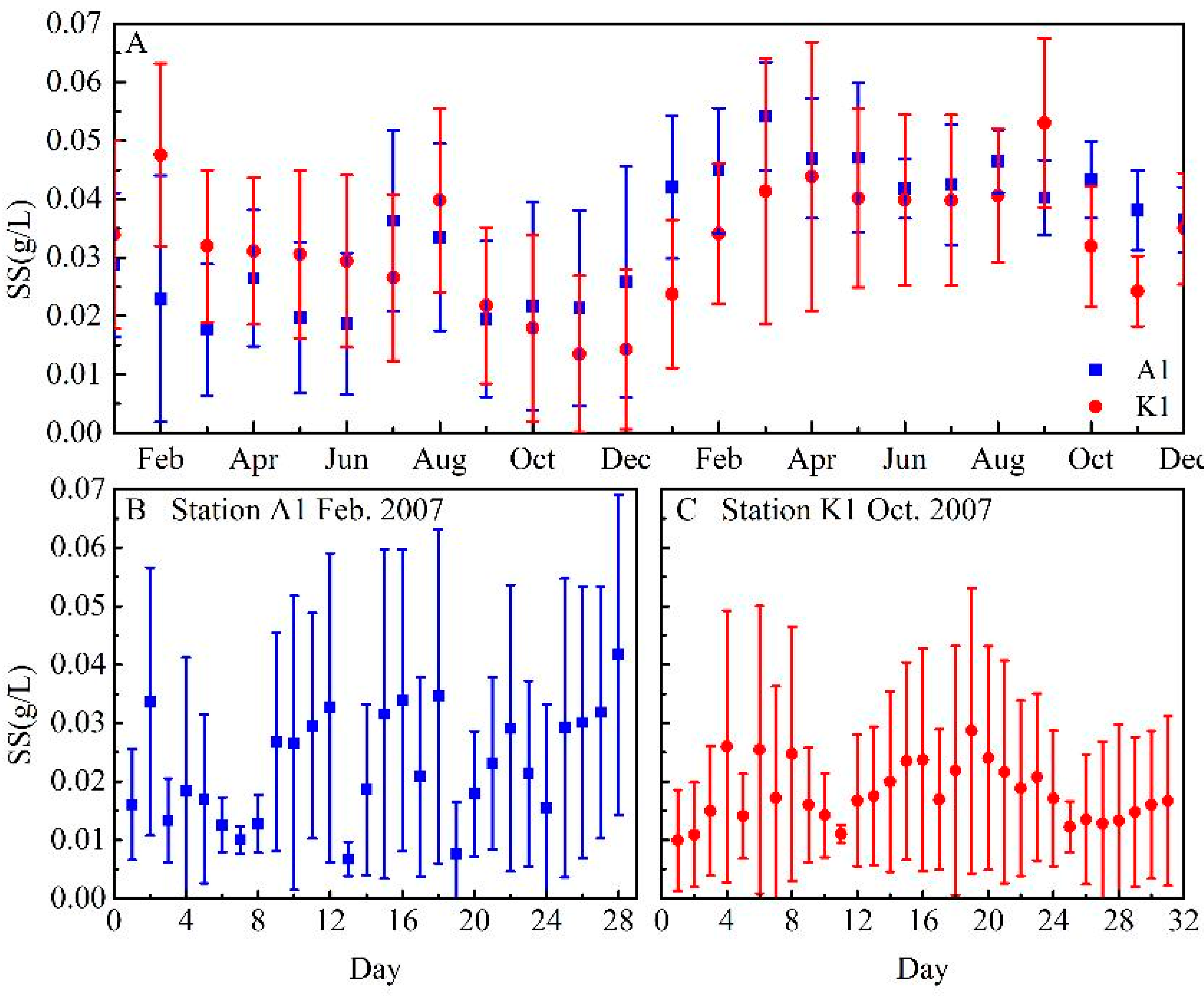
3.1. Temporal Variations of SS

Significant temporal variations of SS in Deep Bay were observed from the two-year continuous time series data. Five statistical indicators were employed to obtain the general information of the SS without considering the missing data, including the mean, the maximum, the minimum, the STD, and the standard deviation coefficient (SDC).

Table 1. Summary statistics for the suspended sediment (SS) data at stations A1 and K1 in 2007 and 2008. STD, standard deviation; SDC, standard deviation coefficient.

Station and Year	Mean SS (g/L)	Max SS (g/L)	Min SS (g/L)	STD (g/L)	SDC (%)
A1 (2007 and 2008)	0.034	0.118	<10−4	0.017	48.94
A1 (2007)	0.024	0.118	<10−4	0.017	67.59
A1 (2008)	0.044	0.109	0.023	0.010	22.94
K1 (2007 and 2008)	0.033	0.129	<10−4	0.018	54.07
K1 (2007)	0.028	0.106	<10−4	0.017	62.00
K1 (2008)	0.037	0.129	0.008	0.017	44.83

presents these statistical indicators of SS in 2007 and 2008 at stations A1 and K1. The mean values at A1 and K1 were 0.034 and 0.032 g/L, respectively, and the SDCs at the two stations were 48.94% and 54.07%, respectively, indicating that the variation of SS at the two stations was similar. However, the SDCs at A1 and K1 in 2007 were 67.59% and 62.00%, respectively, while those in 2008 were 22.94% and 44.83%, respectively. This indicates that the SS varied more strongly in 2007 than in 2008.

The SS varied greatly in Deep Bay. Figure 7 shows the mean and STD of the SS. Note that the STD in most months was relatively large compared with the mean value. The ratios of the maximum to the minimum SSC in a day varied from 1.2 to 66. The mean SSC varied considerably between different months and the STD of monthly SS data was also large. This indicates that the SS in Deep Bay is dynamic and changes greatly during a month (or even within a day, not presented here), and thus observing SS requires high-frequency measurements. Overall, the SS in 2008 was higher than that of 2007 at both stations.

3.2. Key Factors Influencing SS Variations

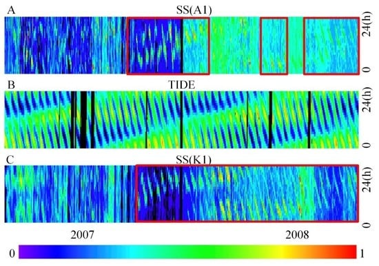
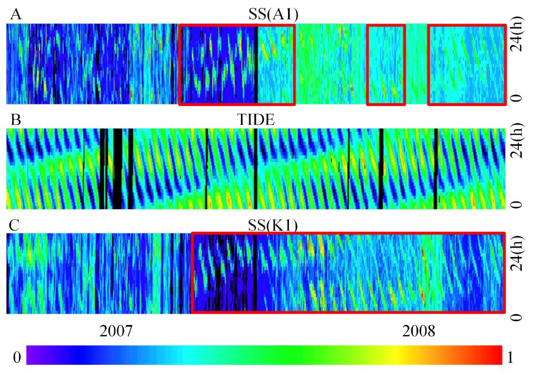
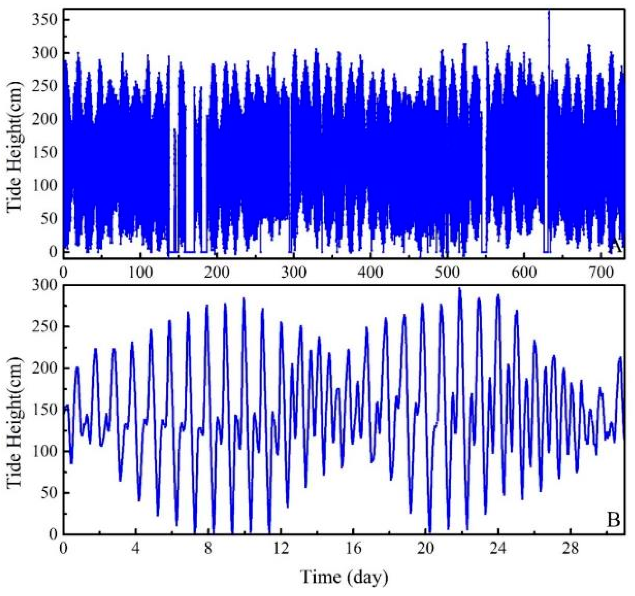
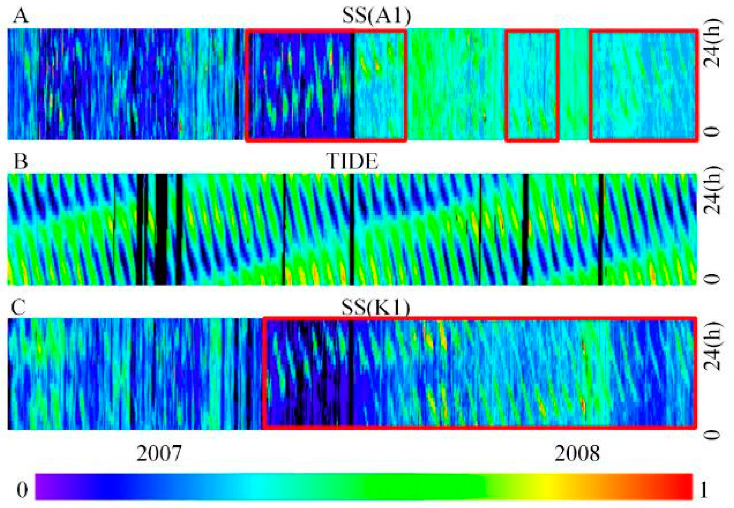
3.2.1. Dominant Impacts of Tide on the SS Temporal Pattern

The raster time series images of SS and tide are shown together in Figure 8. In general, similar temporal patterns of SS and tide were observed from concurrent measurements from 2007 to 2008. The temporal variations of SS were influenced by the tidal cycle, and significant time lag was revealed between the maximum SSC and THW. The regular variation pattern of SS was found to be approximately the same as that of the tide (marked with red frames in Figure 8). The time at which maximum SSC occurred each day showed a strong relationship with the occurrence of the THW or TLW.

Cross-correlation analysis was employed to obtain a quantitative description of the relationship between SS and tide (

Table 2. Cross-correlation results between suspended sediment concentration (SSC) and the tide.

Correlation Coefficient	Frequency (%)	Lag Time (h)	Frequency (%)
<0.6	0.43	≤−5	11.41
0.6–0.7	6.12	−4 to −1	3.73
0.7–0.8	22.77	0	56.77
0.8–0.9	48.56	1 to 4	13.70
0.9–1	22.12	≥5	14.39

). More than 90% of the SS measurements showed a substantial correlation with tidal variations, with a correlation coefficient larger than 0.7. Furthermore, more than 70% of correlation coefficients were larger than 0.8. The lag time between SS and tidal time series measurements reaching the maximum correlation coefficient was also calculated. For about 57% of the measurements, the SS and tidal data reached the maximum correlation coefficient at almost the same time, with a time lag of 0 h. It is noteworthy that about 20% of the data showed the maximum correlation coefficient with a time lag larger than 5 h.

The relationship between SSC and Wind, SSC and Rainfall were analyzed. The cross-correlation between SSC and wind are shown in

Table 3. Cross-correlation results between suspended sediment concentration (SSC) and wind, SSC, and rainfall.

SSC vs. Wind		SSC vs. Rainfall
Correlation Coefficient	Frequency (%)	Correlation Coefficient	Frequency (%)
<0.6	41.06	<0.6	60.64
0.6–0.7	25.21	0.6–0.7	19.45
0.7–0.8	22.55	0.7–0.8	11.54
0.8–0.9	9.64	0.8–0.9	6.35
0.9–1	1.54	0.9–1	2.02

, which shown about 76% of the data with the correlation coefficient smaller than 0.7, and therefore the SSC were less affected by the wind speed. The cross-correlation analysis between SSC and Rainfall were performed using available rainfall data during in situ data collection, and about 80% of the data were found with the correlation coefficient smaller than 0.7. In conclusion, the effect of wind speed and rainfall on the variation of the SSC were not as significant as the impact of tide. Therefore, it is reasonable to infer that while most of the SS variation was determined by the tidal cycle, there were still other factors influencing the SS in Deep Bay. For instance, measurements of SS with irregular temporal patterns in Figure 8, showed an inconsistent trend with the tide. Concurrent meteorological data with SS are analyzed in the following section to reveal factors that may influence the SS variation.

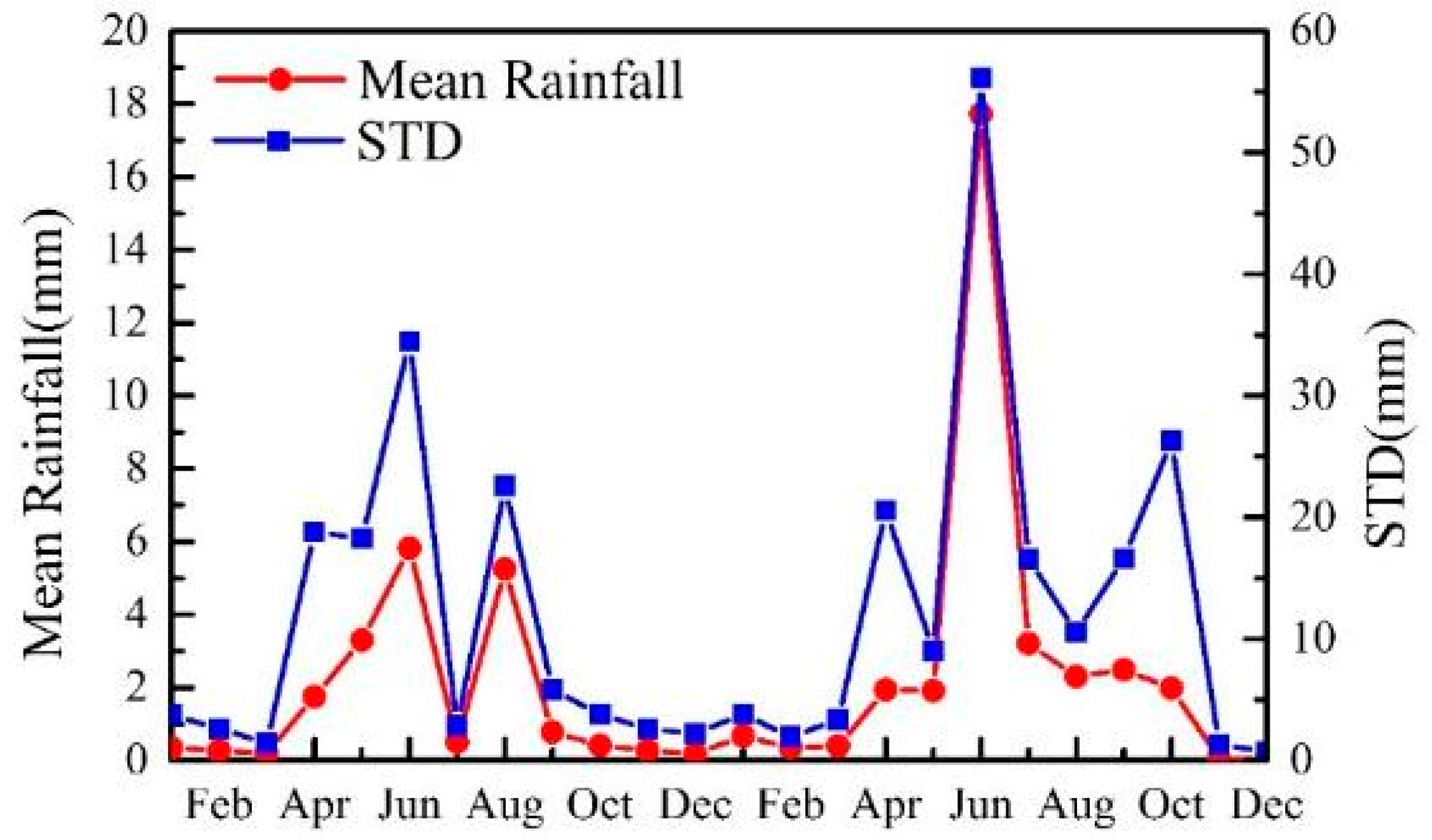
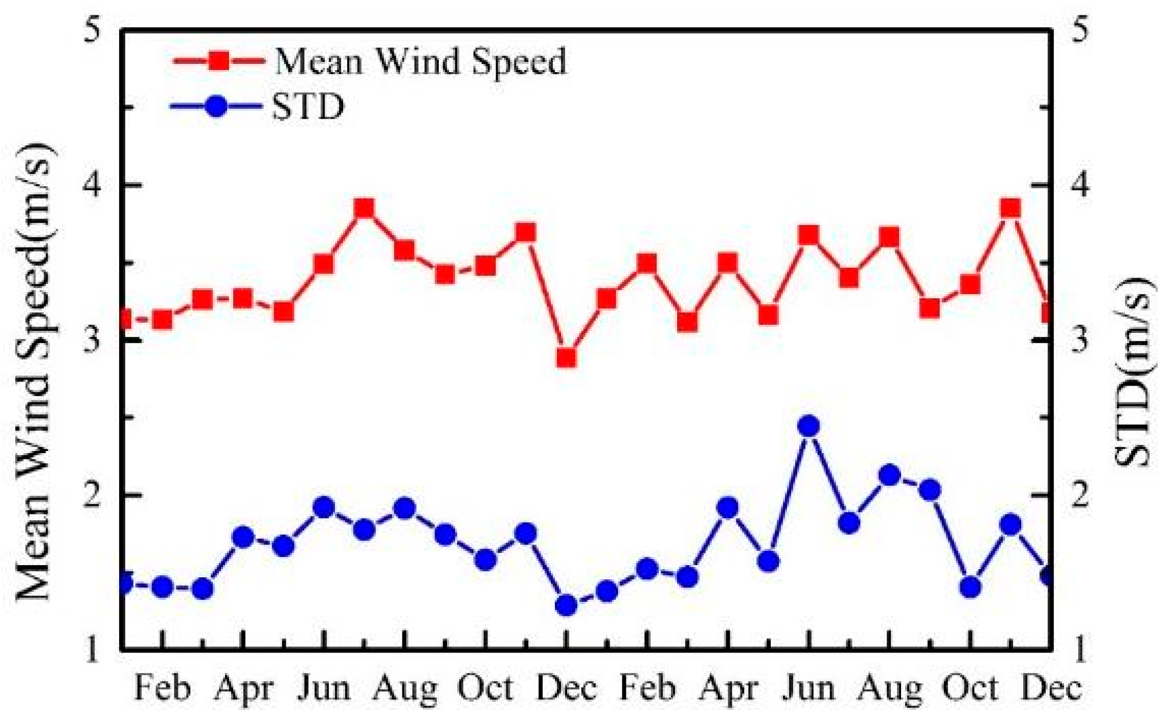
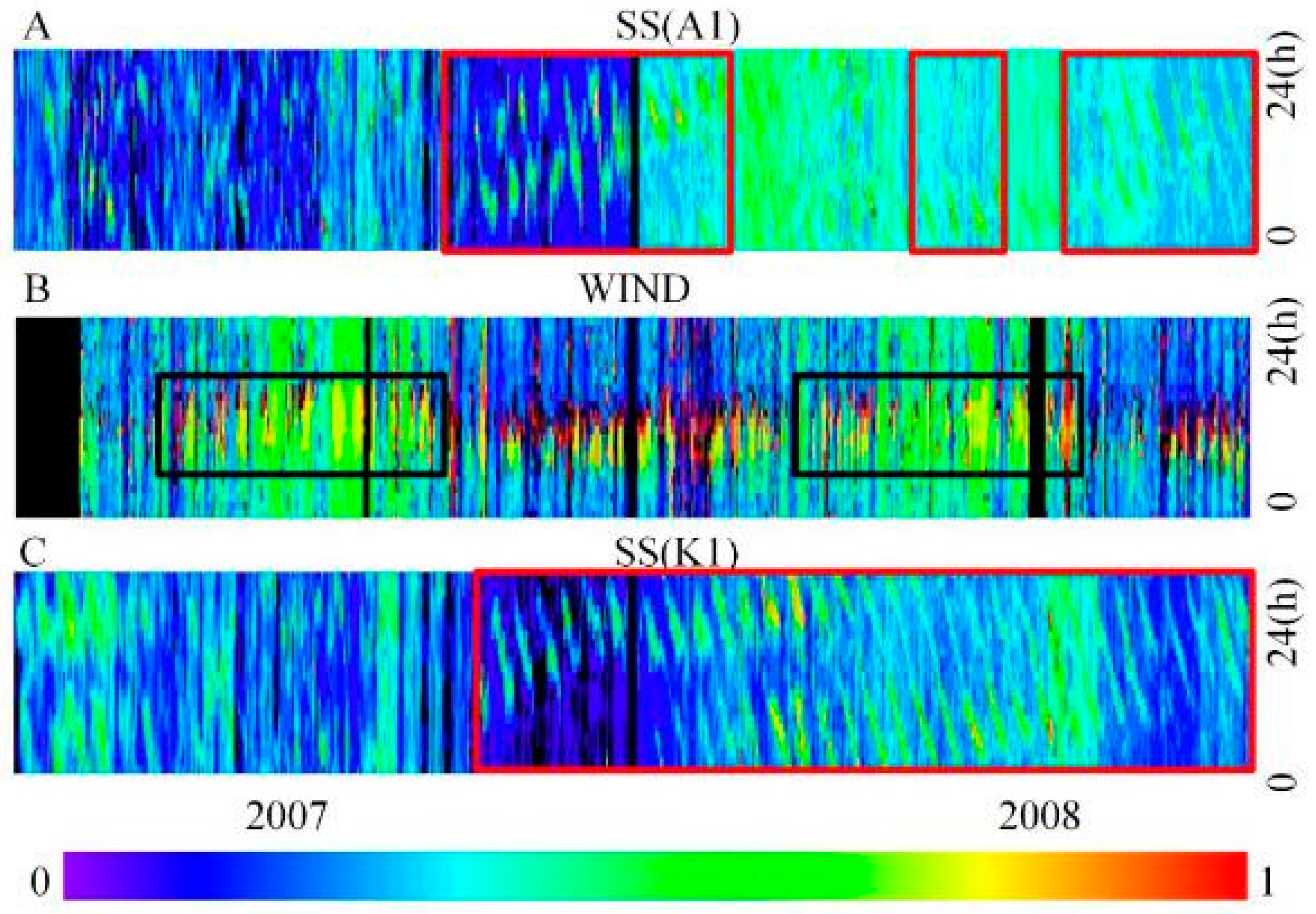
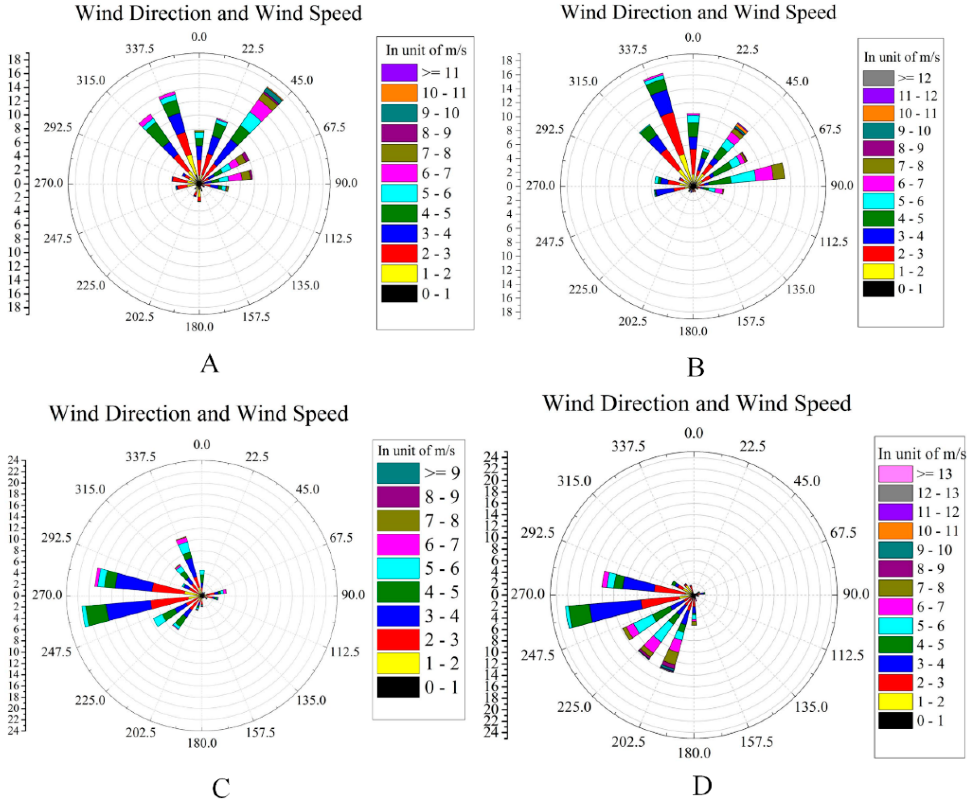
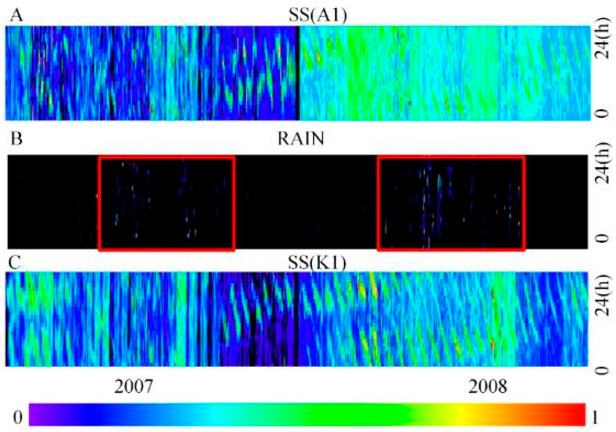
3.2.2. Effects of Meteorological Factors

The main meteorological factors that may affect the SS variation in Deep Bay were analyzed, including wind speed, wind direction and rainfall (Figure 9). Some periods of SS were identified that exhibited variations with regular patterns (red frames in Figure 9). Periods of high wind speeds, corresponded to SS data with both regular and irregular temporal pattern (black frames in Figure 9). This suggests that the wind speed may not be a main influencing factor on the variation of SS.

However, wind has two parameters: wind speed and wind direction. To obtain a deeper understanding of how wind influences the sediment, wind direction was also considered. Two typical cases, both under high wind speed conditions (>4 m/s) were selected to analyze the impacts of wind direction. Case 1 (June 2007 and July 2008) includes periods in which the SS showed a regular variation, and Case 2 (March 2007 and November 2008) was selected to represent an irregular variation of SS (Figure 10).

It is noteworthy that the wind speed and tide were comparable under both cases, whereas the temporal pattern of SS variation was different. Figure 10 provides wind roses for June 2007 and July 2008 (Case 1, regular SS variation), and for March 2007 and November 2008 (Case 2, irregular SS variation). The wind direction under the two different cases showed a substantial discrepancy. For Case 1, the prevailing wind direction was from 337.5° to 90°, whereas for Case 2, the prevailing wind direction was between 180° and 292.5°.

Given the location of Deep Bay (Figure 1), the wind direction from 337.5° to 90° is blowing from the ocean to the bay and wind direction from 180° to 292.5° is the opposite case. This indicates that the influence of wind on SS is related to the wind direction.

Furthermore, the potential influence of rainfall on SS variation was analyzed using the same method. Figure 11 reveal that the rainfall in Deep Bay was concentrated from May to August, and there were no significant changes of rainfall between 2007 and 2008. During the monsoon season in Deep Bay, no evidence was found to demonstrate that the SS variation was directly affected by rainfall.

It is reasonable to conclude that the variation of SS was dominated by the tidal cycle, since the correlation coefficient between SS and tide was larger than 0.7 for >90% of cases. Although the wind speed, wind direction and rainfall can have a certain influence on SS variation, they were restricted in spatial and temporal range.

3.3. Statistical Indicators for SS Sampling Strategy

Statistical indicators are the most common and widely used method to quantitatively describe the status and trend of SS, particularly maximum and minimum values. The maximum and minimum SSC can provide direct measurements of the range and the extreme values of the water quality. Hence, in this section, the optimal sampling time to obtain the most reliable SS measurements was revealed based on a statistical approach. The frequency of the time intervals between the maximum or the minimum SSC and the THW or TLW were calculated, then a frequency histogram was used to analyze the relationships between SS and the tide.

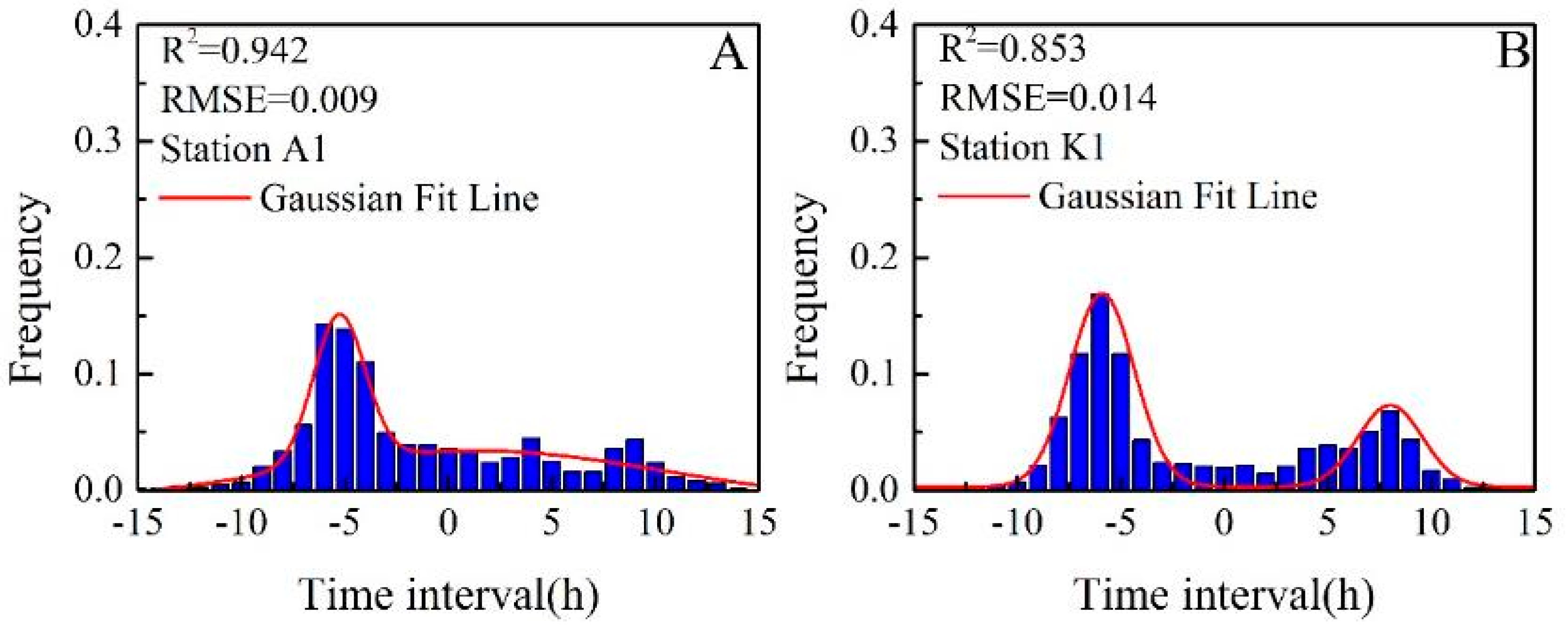
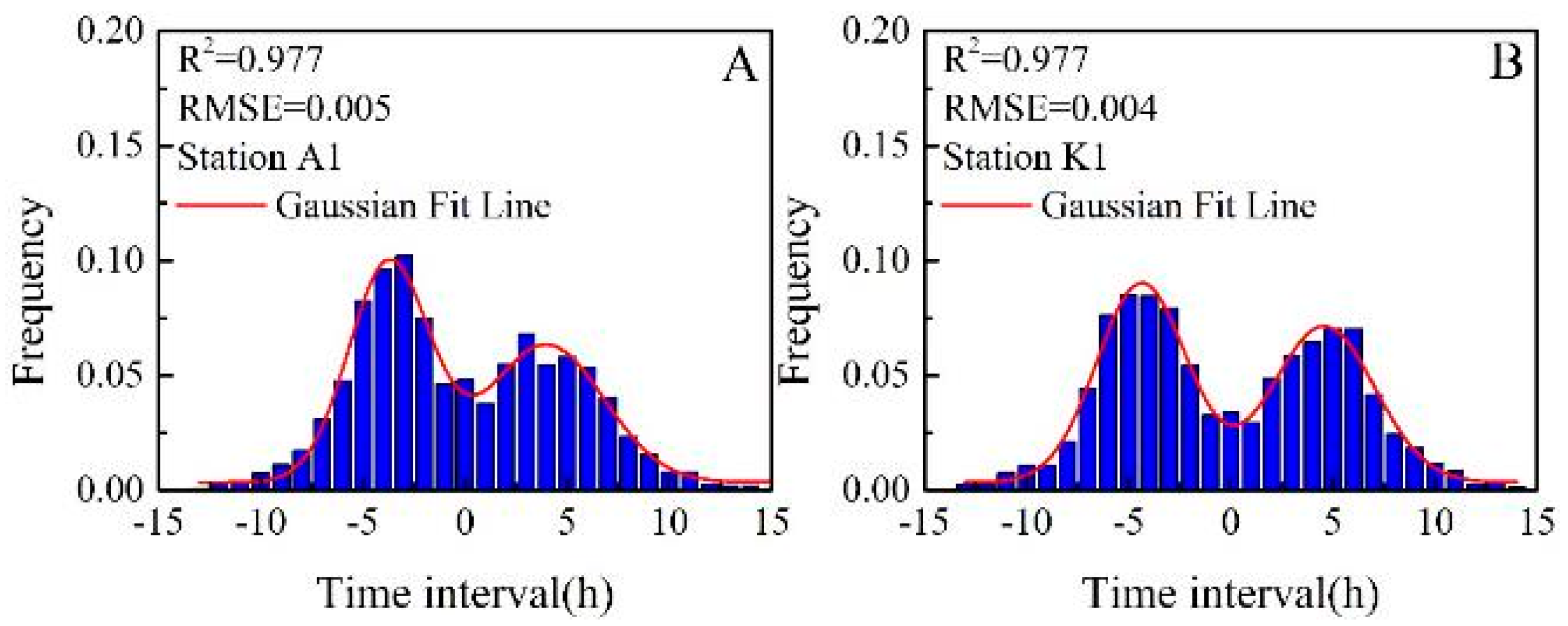
3.3.1. The Maximum SSC and the Tide

The time interval between the maximum SSC and the THW is shown in Figure 12. The histogram peaks were located at about −5 h for both A1 and K1 stations, which indicates that the maximum SSC occurs 5 h ahead of the THW. Furthermore, secondary peaks were also found at about +7 h, which were much smaller. The interval between these two peaks is about 12 h, which was mainly caused by the semidiurnal tidal cycle of Deep Bay.

Gaussian fitting was employed to quantitatively analyze the data distribution of the time interval frequency (

Table 4. Gaussian fit results of the frequency between the time of maximum SSC and THW or TLW.

Site	Parameters	Number	${\mathit{R}}^2$	Mean Values (h)	RMSE	p Value
A1	Max SSC and THW	890	0.942	−5.3	0.009	***
K1	Max SSC and THW	975	0.853	−5.9	0.014	***
A1	Min SSC and TLW	883	0.924	0.5	0.014	***
K1	Min SSC and TLW	970	0.988	0.3	0.007	***

*** means the p value < 0.01.

). The $R^2$ of the four fitted lines was generally larger than 0.85, and the P values were extremely small (marked with three asterisks), indicating that the results of the Gaussian fit are valid. The mean value of the fitted Gaussian distribution of the time interval was about −5.3 and −5.9 h between the maximum SSC and THW at stations A1 and K1, respectively. However, since there were two peaks in the Gaussian fitted lines, it was difficult to determine the maximum SSC from the time of THW.

The same approach was employed to analyze the relationship between the maximum SSC and the TLW. Figure 13 demonstrates a high consistency of the maximum SSC and the TLW. The time interval peaked around 0 h for both A1 and K1 stations. The Gaussian fit model passed the significance testing, and the fitted line was a skinny bell curve and thin tails, which represents a highly concentrated data distribution. This indicates that sampling for the maximum SSC should take place at the TLW.

Table 4 also presents the Gaussian fit results of the time interval between the minimum SSC and TLW at stations A1 and K1. The mean values of the fitted distribution were about 0.5 and 0.3 at stations A1 and K1, respectively. Compared with the results of maximum SSC and the THW, the variation of the SS at Deep Bay was strongly related to the periodic changes of the TLW. The frequency of the time interval between maximum SSC and the TLW was strongly unimodal, and mean values of both site were consistent and stable for each site. This supports the previous assessment that sampling for the maximum SSC should take place at the TLW.

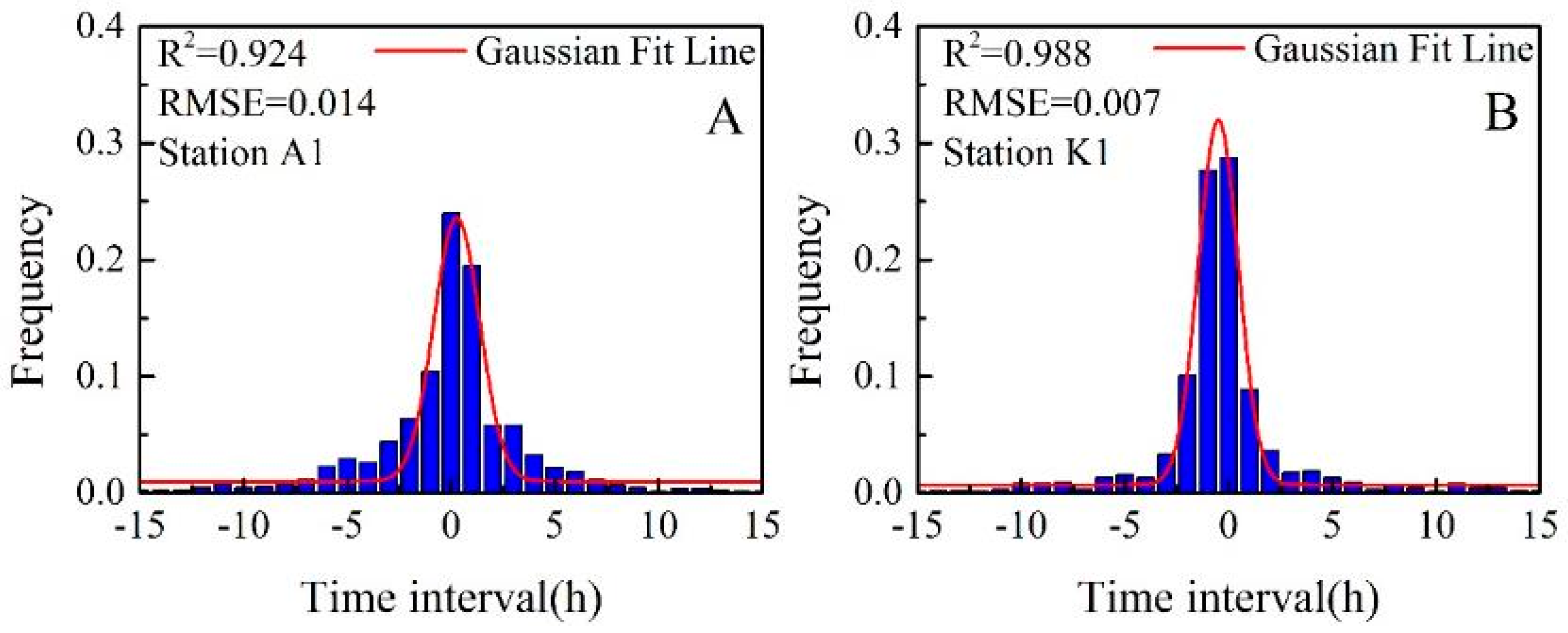
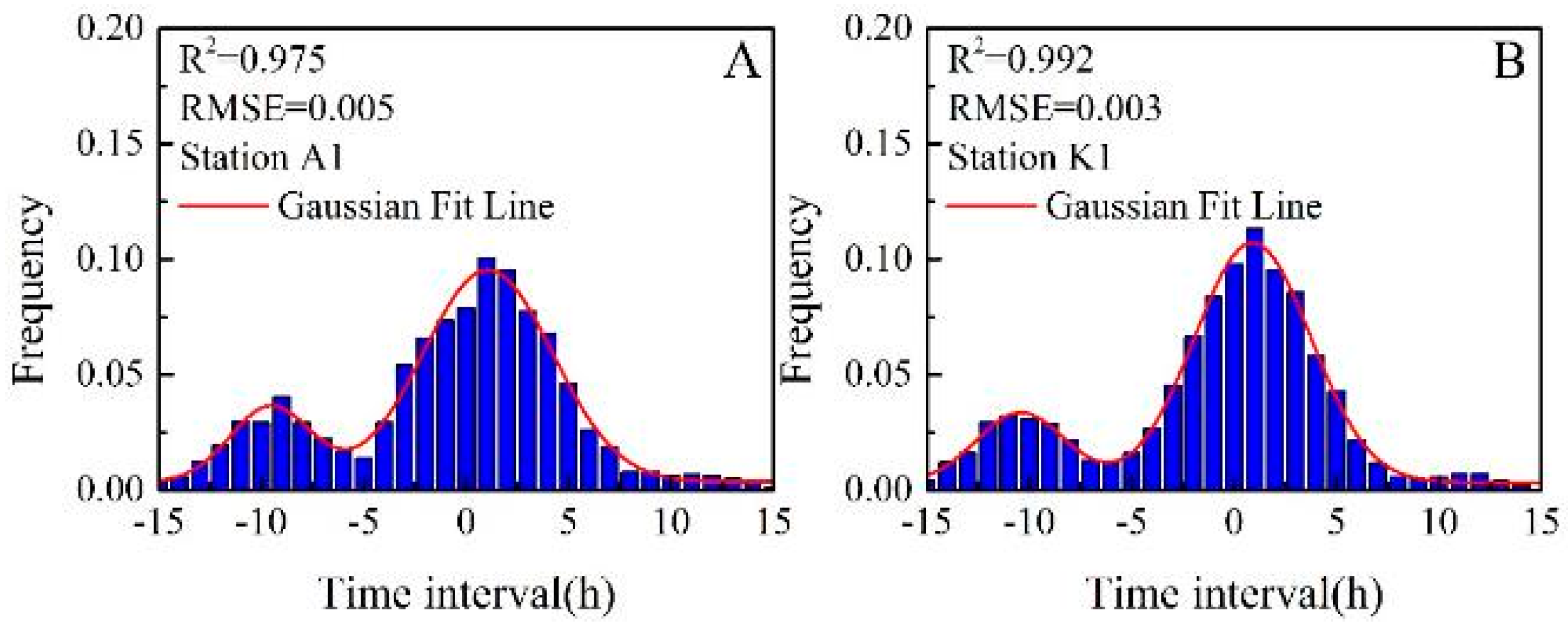
3.3.2. The Minimum SSC and the Tide

The frequency distribution of time intervals between minimum SSC and THW were more dispersed than those between maximum SSC and THW. Similarly, considering the relationship between minimum SSC and THW, there were two peaks of time interval and one was higher than the other. The histogram peaks were found at about −4.1 and 4.7 h for station A1, and −4.2 and 4.8 h for station K1 (

Table 5. Gaussian fit results of the frequency between the time of minimum SSC and THW or TLW.

Site	Parameters	Number	${\mathit{R}}^2$	Mean Values (h)	RMSE	p Value
A1	Min SSC and THW	1616	0.977	−4.9, 4.9	0.005	***
K1	Min SSC and THW	1562	0.977	−4.7, 4.8	0.004	***
A1	Min SSC and TLW	1609	0.975	−9.5, 1.1	0.005	***
K1	Min SSC and TLW	1563	0.992	−10.4, 0.9	0.003	***

*** means the p value < 0.01.

). This indicates that the minimum SSC occurs about 4 h before or 5 h after the THW. The interval between the two peaks was approximately 10 h (Figure 14). The results were also confirmed by the Gaussian fit method and passed the significance tests (Table 5).

Similar results were observed between the minimum SSC and the TLW (Figure 15). Two histogram peaks, with about 12 h interval, were found for both stations, and the time of both two peaks at the two sites were also similar (about −10 h for the first peak and 1 h for the second peak). This indicates that the minimum SSC occurs about 10 h before or 1 h after the TLW. The interval between these two peaks was about 12 h, which was mainly caused by Deep Bay’s semidiurnal tidal cycle.

Therefore, different sampling strategies should be applied when different SS indicators are required. For the monitoring of maximum SSC, the TLW should be selected as an indicator, and the optimum sampling time is recommended to coincide with the TLW. However, the influence of the tide on the minimum SSC was more complex, and multiple sampling times are recommended including about 4 h before or 5 h after the THW, or either 10 h before or 1 h after the TLW. Detailed discussion of the determination of the sampling time is provided in the following section.

4. Discussion

4.1. Resolving the Main Factors Influencing SS

Overall, sediment resuspension and transport caused by wind-driven disturbances and strong tidal currents are frequently observed in shallow water ecosystems [53,54]. The hydrodynamic and meteorological factors have been found to be the main driving forces for the SS variation at both short (minutes) and long (days) time scales [55]. The tidal current or swell would induce resuspension of SS, and thus cause an increase in SS. Similar results have been observed from high frequency observations in many shallow estuarine environments, including Deep Bay, the Lower Bay in Brazil and the Cleveland Bay in Australia and Winyah Bay estuary in USA [42,56,57,58]. In San Francisco Bay, the maximum SSC was observed just after the ebb tide, and the ebb tide caused a SS plume offshore [59], which is similar to our results. Although SS can also be affected by wind pulses, water levels, waves, salinity, and currents [60,61], previous research has demonstrated that the wind forcing alone could not account for all sediment resuspension events [42], though the SS will be increased by wind-induced waves even at a high tide. Moreover, salinity is statistically a minor factor affecting SS if the salinity is stable [62], during the monitoring time in [62], the range of salinity was between 30‰ and 32‰. Moreover, erosion will begin if the current velocity is larger than 0.4 m/s [63], which will cause substantial resuspensi.3on. However, typical tidal current velocity in Deep Bay is about 0.1 m/s in the dry season and 0.35 m/s in wet season [64]. The substantial resuspension caused by erosion can therefore be considered a minor factor of the variation of SS.

Taking advantage of the long-term, continuous, and high-frequency measurements of SS and concurrent hydrodynamic and meteorological data, including tide, wind speed and direction, and rainfall in Deep Bay, the temporal pattern and the main factors of SS variations were analyzed for the first time. Results demonstrated that more than 90% of the SS variation was determined by the tidal cycle in Deep Bay, despite some minimal effect of wind and rainfall. Moreover, the time of maximum SSC coincided with the TLW. It has been previously revealed that the SSC is stored during the flood tides and resuspended during the ebb tides [16] and in the study of Umezawa et al. [62], greater suspended particulate matter appeared at low tide in subtidal areas that face offshore without any barrier. These may explain why the maximum SSC occurred at the time of the TLW.

Although the wind speed, wind direction and rainfall had an influence on SS variation, the effects were restricted within a certain spatial and temporal range. During the period in which the variations of SS were not consistent with the movement of the tide, the wind direction showed some impact on SS variation. In particular, wind direction from the ocean to the bay had a stronger influence on SS than that from the bay to the ocean. This may be related to the fact that wave height generally increases when the current is opposite to wind direction, wave height generally increases, enlarging the shear stress on the bottom [63]. Rain storms and total precipitation may also influence the SS in the river mouth or estuary [22], but no significant relationships were found between SS and rainfall at Deep Bay.

Moreover, since some parameters affecting SS were not measured in the field experiments, further improvements are needed to obtain a deeper analysis of those factors. Besides, due to the distance (14.7 km) between tidal measurement site and the SS monitoring sites, there exist periodicity time lag between the tidal variations at SS sites and observed in the tidal site. The tidal current speed in the Deep Bay and Pearl River region reach as high as 1.2 m/s in spring tide and weaken to 0.3 m/s in neap tide [65,66], therefore, the time lag could be estimated to be approximately 3 h. Since the variations of tide is periodic, the effect caused by the distance is systematic and could be predicted using the tidal current speed. However, the results demonstrated that, in Deep Bay, SS variation was mainly determined by the tidal cycle. The results of this study should be very helpful for remote sensing methods to determine the optimal time at which to monitor SS.

4.2. Implications for Optimized SS Sampling Strategy

Although remote sensing observations are representative for the upper part of the water column, and the highest SSC occur near the bed, the variability in SS observed at the surface is likely to be present throughout the water column [59]. Thus, remote sensing could be used to monitor SS. However, both field measurements and remote sensing require an appropriate sampling time to acquire the most credible data. Since field measurements are costly, time- and labor-intensive [30], it is impractical to conduct continuous and high frequency SS measurements. Moreover, for regions with significant diurnal or semidiurnal variations such as Deep Bay, the efficiency and precision of both in situ and satellite observations for SS monitoring are determined by their sampling strategy (time and interval). In most cases only limited measurements (i.e., once a day for in situ or twice a day for remote sensing such as Terra/Aqua MODIS) are available [38,39,40].

Therefore, a better sampling strategy is required to obtain statistically significant data for SS monitoring. The SS is influenced by many factors, especially the tidal cycle (i.e., dramatic variation of SS was observed in Deep Bay) and thus the conventional measurement method with fixed sampling time would introduce high uncertainty. However, since SS in Deep Bay and other similar regions is influenced by the rhythmic and predictable tidal cycle, guidance can be provided for an optimized sampling strategy.

Under normal weather conditions (no heavy rain and wind), which account for about 80% of the observations of an entire year, the maximum SSC should be measured at the time of the TLW. Since Deep Bay has a semidiurnal tide, the tides and currents can be forecasted according to tidal theory. Several methods have been proposed and widely used to predict tide, including Fourier analysis [67] and Harmonic analyses [68] in the past, and the Chaos theory [69] and the artificial neural network method [70,71] more recently.

In harmonic analysis, the tidal level $Y\left(t\right)$ at any place can be defined in terms of a sum of harmonic analysis terms [70]:

$$Y\left(t\right)=A_0+{\displaystyle \sum }_{i=0}^N{h}_{i}cos\left({\omega }_{i}t+{\epsilon }_i\right)$$

(6)

where $A_0$ is the average tide height, $N$ is the total number of constituents and $h_i$, ${\omega }_i$, ${\epsilon }_i$ represent the amplitude, the speed, and the phase of the constituent. Since harmonic analysis involves an adequate number of constituents, Lee et al. [70] applied back-propagation neural network into tidal prediction. The normalized root mean squared error and correlation coefficient of this method is 0.1835 and 0.9309, respectively, based on only 30 days of tide data [70].

Therefore, the tidal analysis is relatively stable and accurate. It is, therefore, possible for us to forecast the tidal motion from historical tidal data measured in past years. As a result, a better sampling time for SS can be developed from the tidal prediction and the relationships between the tidal cycle and SS.

5. Summary and Conclusions

This study focused on the factors influencing SS based on a statistics and image processing perspective. With reference to two years of continuous and high frequency measurements of SS and concurrent tidal and meteorological data, we found that the tide is the dominant factor influencing the SS variation in Deep Bay. For the monitoring of maximum SSCs, the optimum sampling time corresponds with the TLW, and multiple sampling times are recommended for monitoring of minimum SSC. Although variations of SS were also affected by other factors, the recommended sampling strategy could capture the maximum and minimum SSC variations exactly more than 85% days in a year on average in Deep Bay and can be extended to other estuarine or coastal waters with similar climatological/tidal exposures.

The current sampling time of field SS measurements is often random and subjective, which would introduce considerable uncertainty and loss of comparability between different studies. This study provided a baseline of the SS variation and a direct guidance for the SS sampling time. Future research will focus on the mechanism of the tidal movements on the SS variation, and the verification of the framework in other regions. In addition, a synthetic evaluation of the existing sampling method including field measurements and widely used remote sensing approach will be conducted to assess the reliability of historical data.

References

1. Mouw, C.B.; Greb, S.; Aurin, D.; DiGiacomo, P.M.; Lee, Z.; Twardowski, M.; Binding, C.; Hu, C.; Ma, R.; Moore, T.; et al. Aquatic color radiometry remote sensing of coastal and inland waters: Challenges and recommendations for future satellite missions. Remote Sens. Environ. 2015, 160, 15–30. [Google Scholar] [CrossRef]
2. Fernandez, R.L.; Bonansea, M.; Marques, M. Monitoring turbid plume behavior from landsat imagery. Water Resour. Res. 2014, 28, 3255–3269. [Google Scholar] [CrossRef]
3. Hestir, E.L.; Brando, V.E.; Bresciani, M.; Giardino, C.; Matta, E.; Villa, P.; Dekker, A.G. Measuring freshwater aquatic ecosystems: The need for a hyperspectral global mapping satellite mission. Remote Sens. Environ. 2015, 167, 181–195. [Google Scholar] [CrossRef]
4. Dirk, A.; Antonio, M.; Bryan, F. Spatially resolving ocean color and sediment dispersion in river plumes, coastal systems, and continental shelf waters. Remote Sens. Environ. 2013, 137, 212–225. [Google Scholar]
5. Kantamaneni, K.; Du, X.; Aher, S.; Rao, M.S. Building blocks: A quantitative approach for evaluating coastal vulnerability. Water 2017, 9, 905. [Google Scholar] [CrossRef]
6. Giardino, C.; Bresciani, M.; Villa, P.; Martinelli, A. Application of remote sensing in water resource management: The case study of lake Trasimeno, Italy. Water Resour. Manag. 2010, 24, 3885–3899. [Google Scholar] [CrossRef]
7. Morel, A.; Prieur, L. Analysis of variations in ocean color. Limnol. Oceanogr. 1977, 22, 709–722. [Google Scholar] [CrossRef]
8. Zhang, L.; Wang, L.; Yin, K.; Lü, Y.; Zhang, D.; Yang, Y.; Huang, X. Pore water nutrient characteristics and the fluxes across the sediment in the pearl river estuary and adjacent waters, China. Estuar. Coast. Shelf. Sci. 2013, 133, 182–192. [Google Scholar] [CrossRef]
9. Viers, J.; Dupré, B.; Gaillardet, J. Chemical composition of suspended sediments in world rivers: New insights from a new database. Sci. Total Environ. 2009, 407, 853–868. [Google Scholar] [CrossRef] [PubMed]
10. Rochellenewall, E.J.; Chu, V.T.; Pringault, O.; Amouroux, D.; Arfi, R.; Bettarel, Y.; Bouvier, T.; Bouvier, C.; Got, P.; Nguyen, T.M. Phytoplankton distribution and productivity in a highly turbid, tropical coastal system (Bach Dang Estuary, Vietnam). Mar. Pollut. Bull. 2011, 62, 2317–2329. [Google Scholar] [CrossRef] [PubMed]
11. Mari, X.; Torréton, J.P.; Trinh, B.T.; Bouvier, T.; Chu, V.T.; Lefebvre, J.P.; Ouillon, S. Aggregation dynamics along a salinity gradient in the bach dang estuary, north vietnam. Estuar. Coast. Shelf. Sci. 2012, 96, 151–158. [Google Scholar] [CrossRef]
12. Syvitski, J.P.; Vörösmarty, C.J.; Kettner, A.J.; Green, P. Impact of humans on the flux of terrestrial sediment to the global coastal ocean. Science 2005, 308, 376–380. [Google Scholar] [CrossRef] [PubMed]
13. Shi, Z.; Chen, J.Y. Morphodynamics and sediment dynamics on intertidal mudflats in China (1961–1994). Cont. Shelf Res. 1996, 16, 1909–1926. [Google Scholar] [CrossRef]
14. Le Hir, P.; Roberts, W.; Cazaillet, O.; Christie, M.; Bassoullet, P.; Bacher, C. Characterization of intertidal flat hydrodynamics. Cont. Shelf Res. 2000, 20, 1433–1459. [Google Scholar] [CrossRef]
15. Janssen-Stelder, B. The effect of different hydrodynamic conditions on the morphodynamics of a tidal mudflat in the Dutch Wadden sea. Cont. Shelf Res. 2000, 20, 1461–1478. [Google Scholar] [CrossRef]
16. Meade, R.H.; Dunne, T.; Richey, J.E.; Santos, U.D.M.; Salati, E. Storage and remobilization of suspended sediment in the lower amazon river of brazil. Sciences 1985, 228, 488–490. [Google Scholar] [CrossRef] [PubMed]
17. Dong, L.X.; Guan, W.B.; Chen, Q.; Li, X.H.; Liu, X.H.; Zeng, X.M. Sediment transport in the Yellow Sea and East China Sea. Estuar. Coast. Shelf. Sci. 2011, 93, 248–258. [Google Scholar] [CrossRef]
18. Allison, M.A.; Ramirez, M.T.; Meselhe, E.A. Diversion of Mississippi River water downstream of New Orleans, Louisiana, USA to maximize sediment capture and ameliorate coastal land loss. Water Resour. Manag. 2014, 28, 4113–4126. [Google Scholar] [CrossRef]
19. Vinh, V.D.; Ouillon, S.; Thao, N.V.; Tien, N.N. Numerical simulations of suspended sediment dynamics due to seasonal forcing in the Mekong coastal area. Water 2016, 8, 255. [Google Scholar] [CrossRef]
20. Larcombe, P.; Ridd, P.V.; Prytz, A.; Wilson, B. Factors controlling suspended sediment on inner-shelf coral reefs, Townsville, Australia. Coral Reefs 1995, 14, 163–171. [Google Scholar] [CrossRef]
21. Zabaleta, A.; Martínez, M.; Uriarte, J.A.; Antigüedad, I. Factors controlling suspended sediment yield during runoff events in small headwater catchments of the Basque country. Catena 2007, 71, 179–190. [Google Scholar] [CrossRef]
22. Nadal-Romero, E.; Regüés, D.; Latron, J. Relationships among rainfall, runoff, and suspended sediment in a small catchment with badlands. Catena 2008, 74, 127–136. [Google Scholar] [CrossRef]
23. Walling, D.E.; Fang, D. Recent trends in the suspended sediment loads of the world’s rivers. Glob. Planet. Chang. 2003, 39, 111–126. [Google Scholar] [CrossRef]
24. Fernandez, J.M.; Meunier, J.D.; Ouillon, S.; Moreton, B.; Douillet, P.; Grauby, O. Dynamics of suspended sediments during a dry season and their consequences on metal transportation in a coral reef lagoon impacted by mining activities, New Caledonia. Water 2017, 9, 338. [Google Scholar] [CrossRef]
25. Walling, D.E. Human impact on land–ocean sediment transfer by the world’s rivers. Geomorphology 2006, 79, 192–216. [Google Scholar] [CrossRef]
26. Min, J.-E.; Choi, J.-K.; Yang, H.; Lee, S.; Ryu, J.-H. Monitoring changes in suspended sediment concentration on the southwestern coast of Korea. J. Coast. Res. 2014, 70, 133–138. [Google Scholar] [CrossRef]
27. Choi, J.-K.; Yang, H.; Han, H.-J.; Ryu, J.-H.; Park, Y.-J. Quantitative estimation of suspended sediment movements in coastal region using GOCI. J. Coast. Res. 2013, 165, 1367–1372. [Google Scholar] [CrossRef]
28. Yang, X.; Mao, Z.; Huang, H.; Zhu, Q. Using GOCI retrieval data to initialize and validate a sediment transport model for monitoring diurnal variation of SSC in Hangzhou bay, China. Water 2016, 8, 108. [Google Scholar] [CrossRef]
29. Yuan, Z.; Shao, J.; Chen, X. Spatio-temporal analysis of the suspended sediment concentration in the pearl river estuary and Shenzhen bay based on the information analysis theory. Res. Sci. 2009, 31, 1415–1421. [Google Scholar]
30. Glasgow, H.B.; Burkholder, J.A.M.; Reed, R.E.; Lewitus, A.J.; Kleinman, J.E. Real-time remote monitoring of water quality: A review of current applications, and advancements in sensor, telemetry, and computing technologies. J. Exp. Mar. Biol. Ecol. 2004, 300, 409–448. [Google Scholar] [CrossRef]
31. Zolfaghari, K.; Duguay, C. Estimation of water quality parameters in lake Erie from Meris using linear mixed effect models. Remote Sens. 2016, 8, 473. [Google Scholar] [CrossRef]
32. Joshi, I.D.; D’Sa, E.J.; Osburn, C.L.; Bianchi, T.S.; Dong, S.K.; Oviedo-Vargas, D.; Arellano, A.R.; Ward, N.D. Assessing chromophoric dissolved organic matter (CDOM) distribution, stocks, and fluxes in Apalachicola bay using combined field, viirs ocean color, and model observations. Remote Sens. Environ. 2017, 191, 359–372. [Google Scholar] [CrossRef]
33. Ritchie, J.C.; Zimba, P.V.; Everitt, J.H. Remote sensing techniques to assess water quality. Photogramm. Eng. Remote Sens. 2003, 69, 695–704. [Google Scholar] [CrossRef]
34. Wang, Y.; Xia, H.; Fu, J.; Sheng, G. Water quality change in reservoirs of Shenzhen, China: Detection using Landsat/TM data. Sci. Total Environ. 2004, 328, 195. [Google Scholar] [CrossRef] [PubMed]
35. Feng, L.; Hu, C.; Chen, X.; Cai, X.; Tian, L.; Gan, W. Assessment of inundation changes of Poyang lake using Modis observations between 2000 and 2010. Remote Sens. Environ. 2012, 121, 80–92. [Google Scholar] [CrossRef]
36. Matthews, M.W.; Bernard, S.; Robertson, L. An algorithm for detecting trophic status (Chlorophyll-A), cyanobacterial-dominance, surface scums and floating vegetation in inland and coastal waters. Remote Sens. Environ. 2012, 124, 637–652. [Google Scholar] [CrossRef]
37. Chen, J.; Quan, W.; Cui, T.; Song, Q. Estimation of total suspended matter concentration from Modis data using a neural network model in the china eastern coastal zone. Estuar. Coast. Shelf Sci. 2015, 155, 104–113. [Google Scholar] [CrossRef]
38. Choi, J.-K.; Park, Y.J.; Ahn, J.H.; Lim, H.-S.; Eom, J.; Ryu, J.-H. GOCI, the world’s first geostationary ocean color observation satellite, for the monitoring of temporal variability in coastal water turbidity. J. Geophys. Res. Oceans 2012, 117, 4–9. [Google Scholar] [CrossRef]
39. Kaufman, Y.J.; Remer, L.A.; Tanre, D.; Li, R.R.; Kleidman, R.; Mattoo, S.; Levy, R.C.; Eck, T.F.; Holben, B.N.; Ichoku, C. A critical examination of the residual cloud contamination and diurnal sampling effects on modis estimates of aerosol over ocean. IEEE Trans. Geosci. Remote Sens. 2005, 43, 2886–2897. [Google Scholar] [CrossRef]
40. Racault, M.F.; Sathyendranath, S.; Platt, T. Impact of missing data on the estimation of ecological indicators from satellite ocean-colour time-series. Remote Sens. Environ. 2014, 152, 15–28. [Google Scholar] [CrossRef]
41. Gregg, W.W.; Casey, N.W. Sampling biases in Modis and Seawifs ocean chlorophyll data. Remote Sens. Environ. 2007, 111, 25–35. [Google Scholar] [CrossRef]
42. Chen, Z.; Hu, C.; Muller-Karger, F.E.; Luther, M.E. Short-term variability of suspended sediment and phytoplankton in Tampa bay, Florida: Observations from a coastal oceanographic tower and ocean color satellites. Estuar. Coast. Shelf Sci. 2010, 89, 62–72. [Google Scholar] [CrossRef]
43. Qiu, Y.W.; Zhang, G.; Liu, G.Q.; Guo, L.L.; Li, X.D.; Wai, O. Polycyclic aromatic hydrocarbons (PAHS) in the water column and sediment core of deep bay, south China. Estuar. Coast. Shelf Sci. 2009, 83, 60–66. [Google Scholar] [CrossRef]
44. Hun, J.; Wei, L.; Qian, A. In Three-dimensional modeling of hydrodynamic and flushing in deep bay. In Proceedings of the International Conference on Estuaries & Coasts, Hangzhou, China, 9–11 November 2003; pp. 9–11. [Google Scholar]
45. Jie, X.; Yin, K.D.; Lee, J.H.W.; Liu, H.B.; Ho, A.Y.T.; Yuan, X.C.; Harrison, P.J.; Zingone, A.; Phlips, E.J.; Harrison, P.J. Long-term and seasonal changes in nutrients, phytoplankton biomass, and dissolved oxygen in deep bay, Hongkong. Estuar. Coasts 2010, 33, 399–416. [Google Scholar]
46. Xie, H.; Zhou, D.; Pang, X.; Li, Y.; Wu, X.; Qiu, N.; Li, P.; Chen, G. Cenozoic sedimentary evolution of deepwater sags in the Pearl river mouth basin, Northern South China Sea. Mar. Geophys. Res. 2013, 34, 159–173. [Google Scholar] [CrossRef]
47. Tian, L.; Wai, O.; Chen, X.; Liu, Y.; Feng, L.; Li, J.; Huang, J. Assessment of total suspended sediment distribution under varying tidal conditions in deep bay: Initial results from HJ-1A/1B satellite CCD images. Remote Sens. 2014, 6, 9911–9929. [Google Scholar] [CrossRef]
48. Zhang, W.X.; Yang, S.L. Turbidity calibration of Obs and errors analysis of suspended sediment concentration. Ocean Technol. 2008, 4, 5–8. [Google Scholar]
49. Downing, J. Twenty-five years with Obs sensors: The good, the bad, and the ugly. Cont. Shelf Res. 2006, 26, 2299–2318. [Google Scholar] [CrossRef]
50. Zhou, Q.; Tian, L.; Wai, O.; Li, J.; Sun, Z.; Li, W. Impacts of insufficient observations on the monitoring of short- and long-term suspended solids variations in highly dynamic waters, and implications for an optimal observation strategy. Remote Sens. 2018, 10, 345. [Google Scholar] [CrossRef]
51. Papoulis, A. The Fourier Integral and Its Applications; McGraw-Hill: New York, NY, USA, 1962; pp. 159–161. [Google Scholar]
52. Bracewell, R.N. The Fourier Transform and Its Applications; McGraw-Hill: New York, NY, USA, 1965; Volume 31999. [Google Scholar]
53. Alvarez, L.G.; Jones, S.E. Factors influencing suspended sediment flux in the Upper Gulf of California. Estuar. Coast. Shelf Sci. 2002, 54, 747–759. [Google Scholar] [CrossRef]
54. Douglas, R.W.; Rippey, B. The random redistribution of sediment by wind in a lake. Limnol. Oceanogr. 2000, 45, 686–694. [Google Scholar] [CrossRef]
55. Talke, S.A.; Stacey, M.T. Suspended sediment fluxes at an intertidal flat: The shifting influence of wave, wind, tidal, and freshwater forcing. Cont. Shelf Res. 2008, 28, 710–725. [Google Scholar] [CrossRef]
56. Jing, L.; Ridd, P.V. Wave-current bottom shear stresses and sediment resuspension in Cleveland bay, Australia. Coast. Eng. 1996, 29, 169–186. [Google Scholar] [CrossRef]
57. Cloern, J.E. Phytoplankton bloom dynamics in coastal ecosystems: A review with some general lessons from sustained investigation of San Francisco bay, California. Rev. Geophys. 1996, 34, 186–202. [Google Scholar] [CrossRef]
58. Patchineelam, S.M.; Kjerfve, B. Suspended sediment variability on seasonal and tidal time scales in the Winyah bay estuary, South Carolina, USA. Estuar. Coast. Shelf Sci. 2004, 59, 307–318. [Google Scholar] [CrossRef]
59. Ruhl, C.A.; Schoellhamer, D.H.; Stumpf, R.P.; Lindsay, C.L. Combined use of remote sensing and continuous monitoring to analyse the variability of suspended-sediment concentrations in San Francisco bay, California. Estuar. Coast. Shelf Sci. 2001, 53, 801–812. [Google Scholar] [CrossRef]
60. Schoellhamer, D.H. Sediment resuspension mechanisms in old Tampa bay, Florida. Estuar. Coast. Shelf Sci. 1995, 40, 603–620. [Google Scholar] [CrossRef]
61. Lawrence, D.; Dagg, M.J.; Liu, H.B.; Cummings, S.R.; Ortner, P.B.; Kelble, C. Wind events and benthic-pelagic coupling in a shallow Subtropical bay in Florida. Mar. Ecol. Prog. Ser. 2004, 266, 1–13. [Google Scholar] [CrossRef]
62. Umezawa, Y.; Komatsu, T.; Yamamuro, M.; Koike, I. Physical and topographic factors affecting suspended particulate matter composition in a shallow tropical estuary. Mar. Environ. Res. 2009, 68, 59–70. [Google Scholar] [CrossRef] [PubMed]
63. Wolanski, E.; Spagnol, S. Dynamics of the turbidity maximum in king sound, tropical western Australia. Estuar. Coast. Shelf Sci. 2003, 56, 877–890. [Google Scholar] [CrossRef]
64. Mao, Q.; Shi, P.; Yin, K.; Gan, J.; Qi, Y. Tides and tidal currents in the pearl river estuary. Cont. Shelf Res. 2004, 24, 1797–1808. [Google Scholar] [CrossRef]
65. Wong, L.; Chen, J.; Xue, H.; Dong, L.; Su, J.; Heinke, G. A model study of the circulation in the pearl river estuary (PRE) and its adjacent coastal waters: 1. Simulations and comparison with observations. J. Geophys. Res. Oceans 2003, 108, 3165. [Google Scholar] [CrossRef]
66. Pan, J.; Gu, Y.; Wang, D. Observations and numerical modeling of the pearl river plume in summer season. J. Geophys. Res. Oceans 2014, 119, 2480–2500. [Google Scholar] [CrossRef]
67. Cartwright, D.; Catton, D. On the fourier analysis of tidal observations. Int. hydrogr. Rev. 1963, 40, 113–125. [Google Scholar]
68. Van Ette, A.; Schoemaker, H. Harmonic Analysis of Tides: Essential Feature and Disturbing Influences; Deltares (WL): Delft, The Netherlands, 1966. [Google Scholar]
69. Sannasiraj, S.A.; Zhang, H.; Babovic, V.; Chan, E.S. Enhancing tidal prediction accuracy in a deterministic model using chaos theory. Adv. Water Resour. 2004, 27, 761–772. [Google Scholar] [CrossRef]
70. Lee, T.L. Back-propagation neural network for long-term tidal predictions. Ocean Eng. 2004, 31, 225–238. [Google Scholar] [CrossRef]
71. Chang, H.K.; Lin, L.C. Multi-point tidal prediction using artificial neural network with tide-generating forces. Coast. Eng. 2006, 53, 857–864. [Google Scholar] [CrossRef]
Figure 1. Location of Deep Bay, China, and in situ sites (A1 and K1, red stars), the tidal measuring station at Tsim Bei Tsui (yellow circle) and meteorological measuring station at Lau Fau Shan (blue triangle). The image is from Landsat/TM observation on 2 November 2009 (RGB = band 5, band 4, band 3).
Water 10 00323 g001
Figure 2. OBS calibration using the in situ mass obtained in water samples.
Water 10 00323 g002
Figure 3. Half-hourly time series of SS (mg/L) at stations A1 and K1 (A) with concurrent time series of tide height (m) at Tsim Bei Tsui (B), wind speed (m/s) and wind direction ( ° ) at Lau Fau Shan (C), and rainfall (mm) at Lau Fau Shan (D). The time shown here is local time (Beijing Time), starting from midnight on 1 January 2007 and ending on midnight on 1 December 2008.
Water 10 00323 g003
Figure 4. The long term and high frequency tide heights in 2007 and 2008 (A) and the tide heights throughout January 2008 (B) at Tsim Bei Tsui in Deep Bay.
Water 10 00323 g004
Figure 5. Monthly mean rainfall and its standard deviation (STD) at Lau Fau Shan meteorological station in 2007 and 2008.
Water 10 00323 g005
Figure 6. Monthly mean wind speed and its STD at Lau Fau Shan meteorological station in 2007 and 2008.
Water 10 00323 g006
Figure 7. Monthly mean suspended sediment (SS) concentrations (points) and their standard deviations (bars) in 2007 and 2008 at stations A1 and K1 (A) and daily mean SS concentrations (points) and their standard deviations (bars) in February 2007 at station A1 (B) and in October 2007 at station K1 (C).
Water 10 00323 g007
Figure 8. Raster image of suspended sediment (SS) at stations A1 (A) and K1 (C) and tide (B) in 2007 and 2008. The row of each part represents the 24 h in a day and the column of each image covers the 731 days of two years of measurements. The color denotes the normalized value and black sections represent missing data. Data in red frames show measurements of SS at each station that have a highly similar temporal pattern to the tides.
Water 10 00323 g008
Figure 9. Raster image of suspended sediment (SS) at station A1 (A) and K1 (C) and wind speed (B) in 2007 and 2008. The color denotes the normalized values and black sections represent missing data. Red frames in the SS image indicate variations with regular patterns. Wind speed with black frames indicates high wind speed data, which corresponded to SS data with both a regular and irregular temporal pattern.
Water 10 00323 g009
Figure 10. The wind direction and wind speed at June 2007 (A), July 2008 (B), March 2007 (C) and November 2008 (D) at Lau Fau Shan meteorological station.
Water 10 00323 g010
Figure 11. Raster image of suspended sediment (SS) at station A1 (A) and K1 (C) and rainfall (B) in 2007 and 2008. The color denotes the normalized values and black sections represent missing data. Red frames in rainfall image indicate the rainy season.
Water 10 00323 g011
Figure 12. Histogram of the time interval between the maximum SSC and the THW at stations A1 (A) and K1 (B). Thick red lines show the Gaussian fit.
Water 10 00323 g012
Figure 13. Time interval between the maximum SSC and the TLW at Station A1 (A) and K1 (B).
Water 10 00323 g013
Figure 14. Time interval between the minimum SSC and the THW at stations A1 (A) and K1 (B) in 2007 and 2008.
Water 10 00323 g014
Figure 15. The time interval between the minimum SSC and the TLW at stations A1 (A) and K1 (B) in 2007 and 2008.
Water 10 00323 g015