Identification of Hydrological Drought in Eastern China Using a Time-Dependent Drought Index


1
State Key Laboratory of Water Resources and Hydropower Engineering Science, Wuhan University, Wuhan 430072, China
2
Key Laboratory of Water Cycle and Related Land Surface Processes, Institute of Geographic Sciences and Natural Resources Research, Chinese Academy of Sciences, Beijing 100101, China
3
Ministry of Education Key Laboratory for Earth System Modeling, Department of Earth System Science, Tsinghua University, Beijing 100084, China
*
Authors to whom correspondence should be addressed.
Water 2018, 10(3), 315; https://doi.org/10.3390/w10030315
Submission received: 31 January 2018
/
Revised: 12 March 2018
/
Accepted: 12 March 2018
/
Published: 13 March 2018
(This article belongs to the Special Issue Data-Driven Methods for Agricultural Water Management)
Abstract
:Long records (1960–2013) of monthly streamflow observations from 8 hydrological stations in the East Asian monsoon region are modeled using a nonstationarity framework by means of the Generalized Additive Models in Location, Scale and Shape (GAMLSS). Modeling analyses are used to characterize nonstationarity of monthly streamflow series in different geographic regions and to select optimal distribution among five two-parameter distributions (Gamma, Lognormal, Gumbel, Weibull and Logistic). Based on the optimal nonstationarity distribution, a time-dependent Standardized Streamflow Index (denoted SSIvar) that takes account of the possible nonstationarity in streamflow series is constructed and then employed to identify drought characteristics at different time scales (at a 3-month scale and a 12-month scale) in the eight selected catchments during 1960–2013 for comparison. Results of GAMLSS models indicate that they are able to represent the magnitude and spread in the monthly streamflow series with distribution parameters that are a linear function of time. For 8 hydrological stations in different geographic regions, a noticeable difference is observed between the historical drought assessment of Standardized Streamflow Index (SSI) and SSIvar, indicating that the nonstationarity could not be ignored in the hydrological drought analyses, especially for stations with change point and significant change trends. The constructed SSIvar is, to some extent, found to be more reliable and suitable for regional drought monitoring than traditional SSI in a changing environment, thereby providing a feasible alternative for drought forecasting and water resource management at different time scales.
1. Introduction
Drought is an insidious natural hazard that has damaging and costly impacts on agriculture, water resources, ecology, and society [1,2]. Due to global climate change and rapid socio-economic development, drought disasters have occurred more frequently and extensively in recent decades [3]. Drought is commonly defined as below-normal water availability [4] and can be subdivided into different types of drought related to the variables of the hydrological cycle, precipitation (meteorological drought), soil moisture (agricultural drought), and streamflow (hydrological drought) [5].
Hydrological drought is defined as a significant shortage of availability of water in all its forms appearing in the land phase of the hydrological cycle (e.g., streamflow, groundwater level and lake level) [6]. It is traditionally detected using field observations of streamflow, surface water and groundwater levels, thereby providing direct evidence of any below-normal water availability [6,7]. Below-normal water availability in rivers, lakes and reservoirs can cause water scarcity in combination with water demand, threating water supply and associated food production [8]. Thus, it is important to identify hydrological drought characteristics and assess the effects of hydrological drought quantitatively. The Standardized Streamflow Index (SSI), proposed by Shukla and Wood [9], has been used as a useful index for characterizing hydrological drought. It is constructed using streamflow data based on the concept of the standardized precipitation index (SPI). Similar to SPI, with the advantages of computational simplicity, the SSI is capable of characterizing hydrological drought condition at different time scales [3,10], and it enables the severity of hydrological drought in different locations to be compared independently of the local characteristics [11]. In addition, the SSI is sensitive to the factors and assumptions that govern probabilistic hydrology, since it is a probability-based drought index [6].
Generally, statistical inferences and statistical analyses for hydrologic time series have relied heavily on the assumption of stationarity in hydrology [12,13]. Under the stationarity assumption, hydrological series keep their distributional properties invariant with time, implying lack of trends and shift [14]. However, the stationarity assumption has been widely questioned and should no longer serve as a central, default assumption, as a result of global climatic change and man-induced disturbance [15,16,17]. In recent years, hydrological nonstationarity has drawn considerable attention [14,18]. Coulibaly and Baldwin [18] developed an optimal dynamic recurrent neural networks method to directly forecast hydrological series under nonstationarity conditions, and they found that neural networks are good alternatives for modeling the complex dynamics of the hydrological system. Villarini et al. [14] modeled a long record of seasonal rainfall and temperature in a nonstationarity framework to characterize non-stationarities in hydro-climatic variables.
In the traditional calculation of SSI values, the streamflow sample series are firstly fitted to a suitable stationary probability distribution on the basis of stationarity assumption [11]. This means that historical features of streamflow series can be used to derive SSI values in the future. However, changing environments (e.g., climate change and human activities) might alter the statistical characteristics of hydroclimate time series [19], resulting in so-called nonstationarity. With respect to streamflow, there have been numerous studies on individual impacts of climate change (mainly changes in precipitation and temperature) and human activity (mainly water construction and building of dams) on it [20], implying clear violations of the stationarity assumption. Ignoring the nonstationarity would therefore most likely diminish the availability and validity of traditional SSI in hydrological drought analysis and could lead to the underestimation or overestimation of the drought severity [21]. Thus, it is essential to incorporate the nonstationarity of streamflow sample series in constructing an appropriate variant SSI (SSIvar) under nonstationarity conditions, thereby providing significant information for evaluation and mitigation of risk of hydrological drought hazards and management of water resources. From this point of view, although some researchers have attempted to consider nonstationarity in developing drought index for drought monitoring, most research has only focused on mean time variance of precipitation time series for meteorological drought (e.g., [22,23]). However, to date, relatively few studies have addressed the stationarity or nonstationarity of streamflow series for hydrological drought using a nonstationarity framework in different geographic regions considering both trends and change points in the parameters. This constituted the major motivation of this study.
Several methods have been proposed to model nonstationarity time series in the previous literature (e.g., [24,25]), each having their own strengths and weakness. The Generalized Additive Models for Location, Scale and Shape (GAMLSS), proposed by Rigby and Stasinopoulos [26], has recently gained popularity in modeling nonstationarity time series in hydrology [27]. This model provides a high degree of flexibility in addressing nonstationarity probabilistic modeling. In GAMLSS, the assumption that the variable of interest follows a distribution from the exponential family is relaxed, allowing the use of more general distributions, such as highly skewed or kurtotic distributions, which may be more appropriate for modeling the record of interest. This makes it an appealing framework for nonstationarity modeling of hydrometeorological variables to improve the existing drought index.
In this study, the GAMLSS was used to model streamflow with nonstationarity distribution to construct a variant SSI index (SSIvar) in eight catchments in the eastern region of China. The main objectives of this study are: (1) to analyze whether streamflow series are stationary in the eastern region of China, and (2) to construct an appropriate variant SSI that accounts for the changes in the parameters of the selected distribution under nonstationarity conditions. The results of this study could provide important information for the management of water resources and evaluation of hydrological drought hazards under a changing environment.
2. Methodology
2.1. Traditional Standardized Streamflow Index (SSI)
The Standardized Streamflow Index (SSI) was used as the useful counterpart for depicting hydrological aspects of drought. This index has the same theoretical background, transforming monthly streamflow into z-scores. The procedure of traditional SSI calculation is statistically similar to the well-known Standardized Precipitation Index (SPI).
The long-term streamflow series were first fitted to the lognormal distribution (Table 1), as suggested by Nalbantis and Tsakiris [6]. Once the distribution is determined, the SSI (in z-scores) can easily be calculated by following the classical approximation of Abramowitz and Stegun [28]. For example
where is the cumulative distribution function. The constants are C0 = 2.515517, C1 = 0.802853, C2 = 0.010328, d1 = 1.432788, d2 = 0.189269, d3 = 0.001308.
2.2. Change Point and Trend Analysis
2.2.1. Change Point Analysis
As a nonparametric statistical test that allows detection of changes in the mean when the change point time is unknown, the Pettitt test [29] has been suggested by Villarini et al. [12] for analyzing the change point in this study. Mathematically, when a sequence of random variables is divided into two segments represented by and , if each segment has a common distribution function, then the change point is identified at m. The Pettitt test uses a version of the Mann-Whitney statistic (). The breakpoint is defined to be where reaches its maximum value:
The significance level associated with is calculated as
This test is valid for continuous variables, and its null hypothesis is the absence of a change point. If p < 0.05, a significant change point exists.
2.2.2. Temporal Trend Analysis
The Mann-Kendall (M-K) statistical test [30,31] is commonly used for general use in temporal trend analysis due to its robustness for non-normally distributed and censored data, which are frequently encountered in hydro-climatic time series [32]. However, the presence of serial correlation can complicate the identification of trends, in that a positive serial correlation can increase the expected number of false positive outcomes for the Mann-Kendall test. Any serial correlation should be removed before conducting the M-K trend test. Following Zhang et al. [33], the significant trend for the streamflow records was identified using the following steps: (1) compute the lag1 serial correlation coefficient (); (2) if , the M-K test was applied to the streamflow series directly; otherwise (3) the M-K test was applied to the preprocessed time series (). The 95% confidence level was used to evaluate the significance of trends.
2.3. GAMLSS Model
The Generalized Additive Models for Location, Scale and Shape (GAMLSS), proposed by Rigby and Stasinopoulos [26], have been used in our study to model the streamflow series with nonstationarity probability distribution. The GAMLSS assume a parametric distribution for the response variable (streamflow in our study) and model the parameters of the distribution as linear and/or nonlinear, parametric and/or additive nonparametric functions of explanatory variables [12].
A brief description of the GAMLSS model is provided below, with more detailed information available from Rigby and Stasinopoulos [26] and Stasinopoulos and Rigby [34]. In a GAMLSS model, it is assumed that there are independent random variables , for i = 1, …, n, which are fitted to a distribution function of conditional on , a vector of p distribution parameters accounting for location, scale, and shape. Generally, p is less than or equal to four, since one, two, three and four parameter distribution families could provide enough flexibility for most applications in hydrology [35]. The GAMLSS allow for a general distribution function, including highly skewed and/or kurtotic continuous or discrete distributions. The distribution parameters are related to the design matrix of explanatory variables by monotonic link function , for . Similar to Villarini et al. [12], five commonly used two-parameter distributions, i.e., Gamma distribution (GA), Lognormal distribution (LOGNO), Gumbel distribution (GU), Weibull distribution (WEI) and Logistic distribution (LO), were used in this study to model the streamflow series (Table 2). In this study, taking the time as the explanatory variables, the linear functions relating t and parameters (for mean ) and (for variance ) were constructed in the form of:
where and denote the vectors of coefficients of the linear function respectively, and the and is the corresponding constant term.
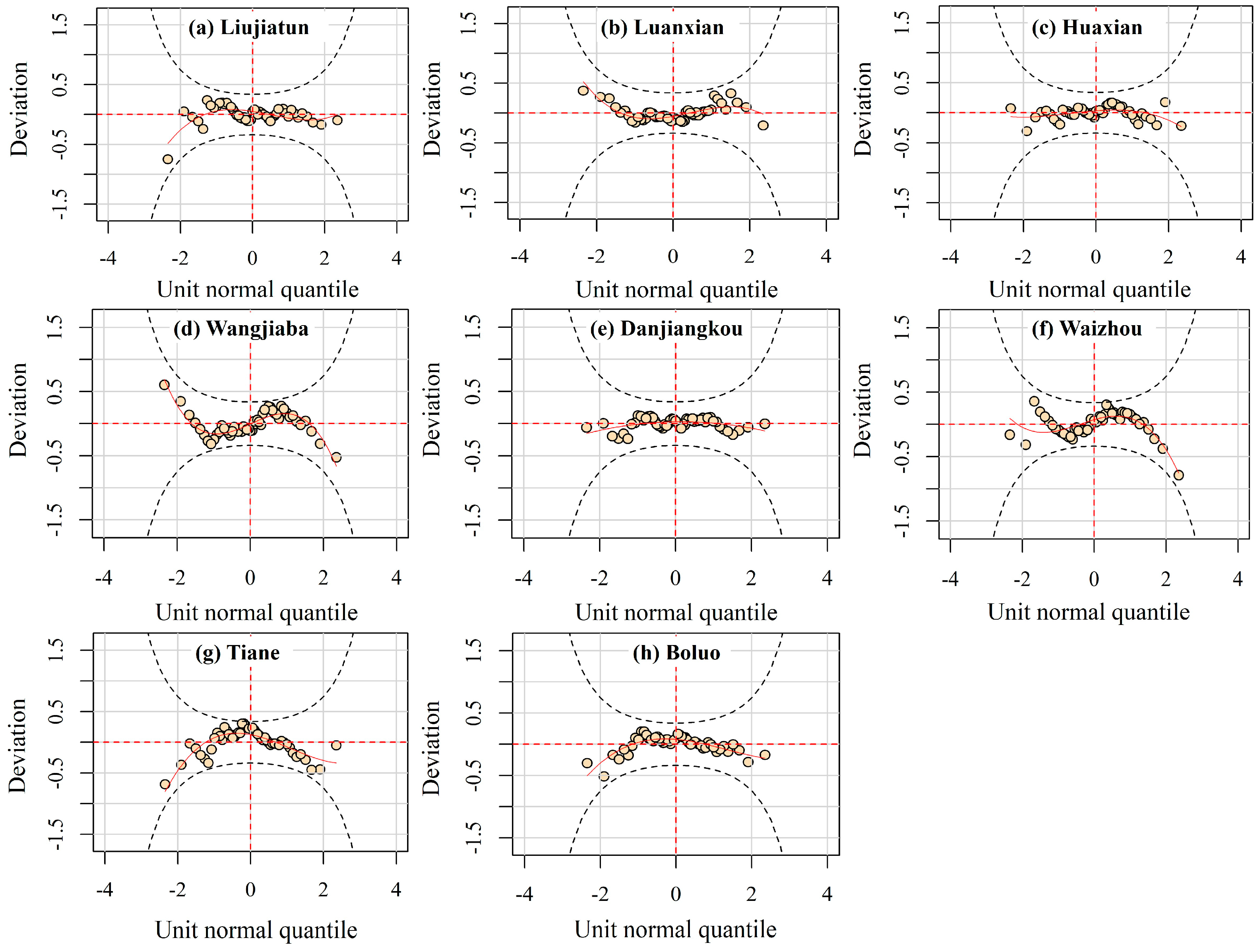
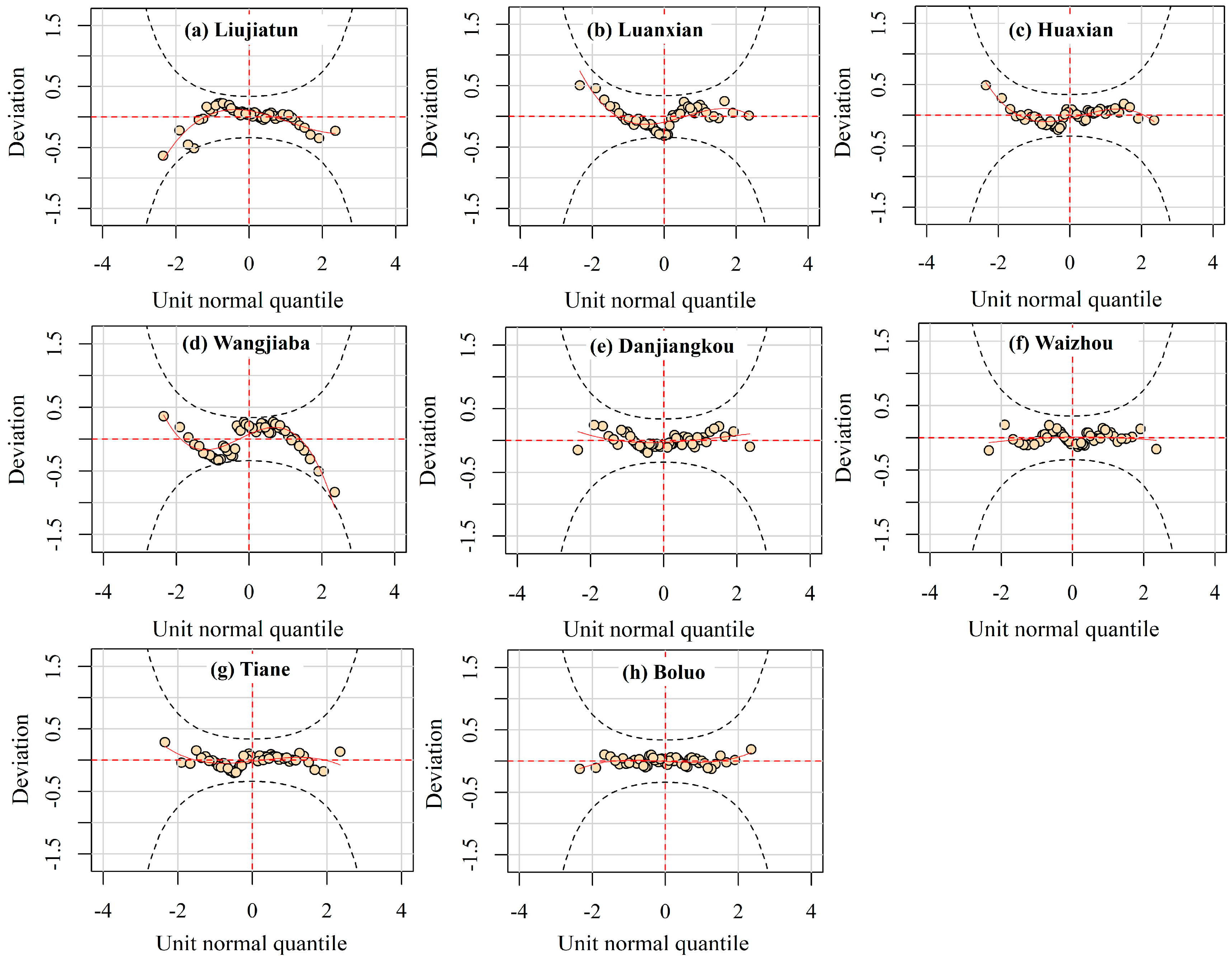
The Akaike Information Criterion (AIC) [36] was used to select the optimal nonstationarity model with the highest goodness-of-fit, and the model with the minimum AIC value was selected. Additionally, to further assess the performance of the selected optimal model, the residuals of each model was checked by the statistics of the Filliben correlation coefficient (denoted by ) [37], together with the worm plot [38] as a visual inspection of diagnostic plots of the residuals. AIC and are calculated as
where ML is the maximum likelihood function of models and k is the number of independently adjusted parameters within the model; are the ordered residuals; n is the length of the observation period and are the standard normal order statistic medians.
Then, based on the GAMLSS, nonstationarity models with different probability distributions, trends in the parameters and the changes point in the time series of streamflow were compared to select an optimal model to construct a newly Standardized Streamflow Index (SSI) for drought monitoring and quantification. Analysis and calculations related to the GAMLSS model in this study were performed with R-based GAMLSS package [34].
2.4. Construction of the Time-Dependent Standardized Streamflow Index (SSIvar)
In our study, to construct a time-dependent Standardized Streamflow Index (SSIvar), the different nonstationarity probability distributions with their parameters changing over time were compared by using GAMLSS, as described in Section 2.3. Considering the long-term trends and abrupt changes can reveal the presence of the nonstationarity in streamflow series. The change points and trends were also included in the analysis by GAMLSS and AIC scores were used to select the optimal models for the Standardized Streamflow Index. Here, synthetic experiments were designed to construct the time-dependent SSI (SSIvar) drought index. Firstly, to select the optimal model for the hydrological stations with no change point, four different models have been analyzed that: (1) stationary model; (2) nonstationarity model in parameter for mean; (3) nonstationarity model in parameter for variance; (4) nonstationarity model in mean and variance. Likewise, for the streamflow series with change points, the study period could be divided into two periods by the change point and four different models are discussed: (1) stationary model; (2) change point only exists in mean; (3) change point only exists in variance; (4) change point exists in both mean and variance.
The constructed SSIvar is calculated in the following steps: (1) calculate the monthly average streamflow () for a given k-month scale (3-month scale and 12-month scale in this study) with respect to time t; (2) within the GAMLSS framework, the nonstationarity model is developed by fitting the streamflow series () to a nonstationarity optimal distribution which is selected by minimizing AIC, then obtaining the corresponding cumulative probability . The parameters of the distribution is described as a linear function of time; (4) the cumulative probability is converted to a standard normal deviate (with zero mean and unit variance), which also using the approximate conversion provided by Abramowitz and Stegun [28]. This standard normal value is the SSIvar index.
Positive values of the SSIvar imply wet conditions, while negative values indicate dry conditions. Since the SSIvar are developed based on the concept of SSI, the classifications listed in Table 2 can be also used for the SSIvar as well. Compared with the traditional SSI, the proposed SSIvar recognize the nonstationarity in the streamflow series and thus it has the ability to capture and model the nonstationarity to provide more reasonable and satisfactory for drought monitoring and drought analysis.
3. Study Area and Dataset
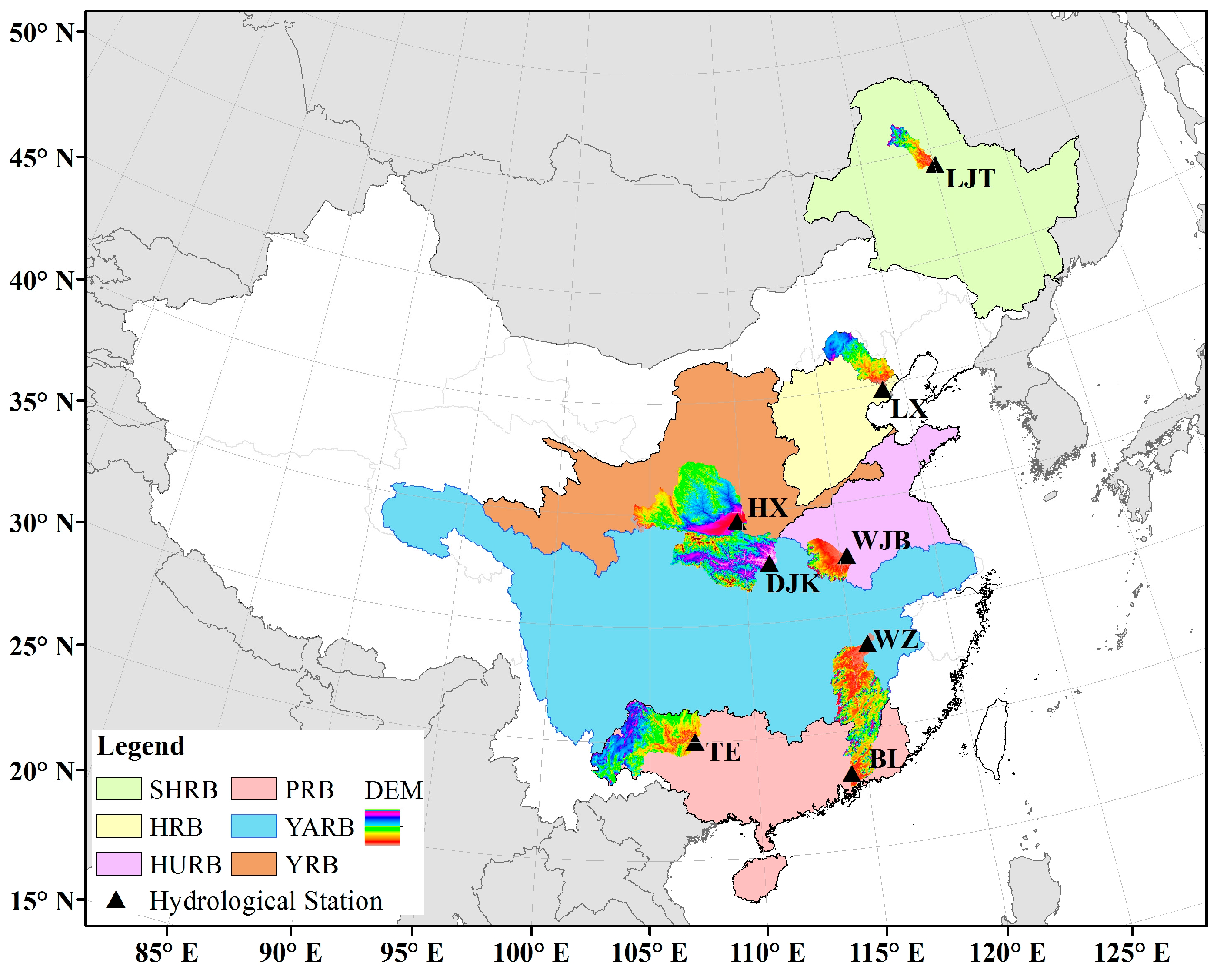
The eastern region of China (the area to the east of 100° E), which is affected by the East Asian monsoon, is usually referred to as the East Asian monsoon (EAM) region. Rainfall mainly occurs in the summer season (June, July and August) in the EAM region. The EAM region is a critically important zone in China, having the densest population and exhibiting the fastest economic development in recent decades. In our study, we selected eight different catchments in the EAM region of China as the case study areas (Figure 1), including Songhua River Basin (SHRB), Hai River Basin (HRB), Yellow River Basin (YRB), Huai River Basin (HURB), Yangtze River Basin (YARB), Pearl River Basin (PRB).
Monthly streamflow records from 1960 to 2013, from eight hydrological stations in different catchments, were analyzed. The data were provided by the Hydrology Bureau of the corresponding River Conservancy Commission. Locations of these stations are shown in Figure 1. Information on the data, such as the length of streamflow series and the drainage areas of hydrological stations, is given in Table 3.
4. Results and Discussion
4.1. Change Point Analysis
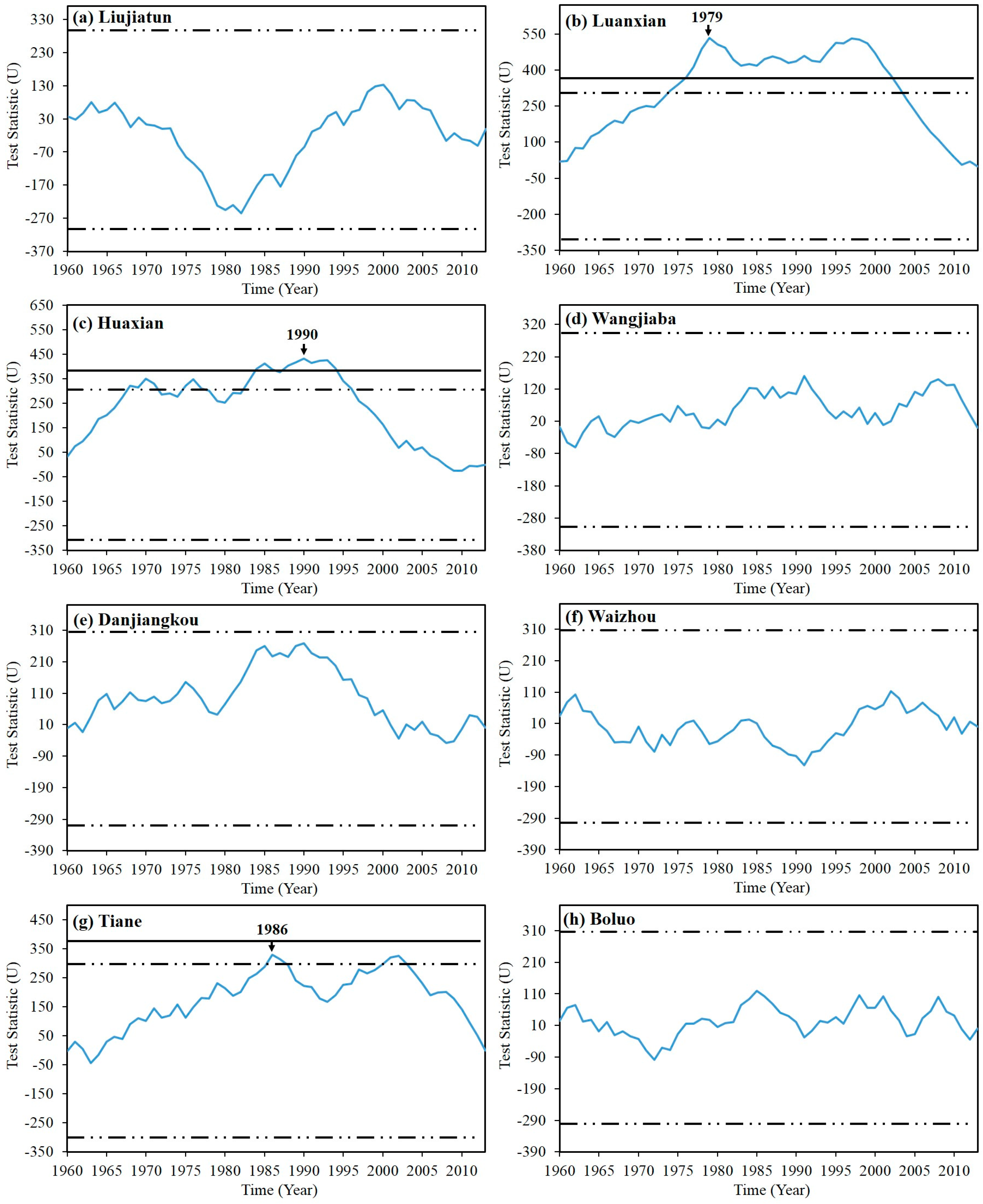
Pettitt’s test was used to detect change points in annual streamflow for the eight selected hydrological stations. The results showed that the annual streamflow in three stations (Luanxian, Huaxian and Tiane) have change points with a significance level of 5% (Figure 2), while the remaining five stations showed no significant change points. The change points for Luanxian, Huaxian and Tiane occurred in 1979, 1990 and 1986, respectively (Figure 2).
4.2. Trend Analysis
Autocorrelation analysis was done first to detect the significant serial effects before trend detection. Apart from Waizhou (lag1 = −0.073) and Boluo (lag1 = −0.066), the lag1 serial correlation coefficient for the other six stations were all beyond the threshold value (0.1) (Table 4), indicating significant effects on trend analysis. The significant autocorrelations in the six stations were removed before the M-K trend test. The results estimated by M-K test are exhibited in Table 4. Among the eight stations, two stations showed an increasing trend and the other six stations demonstrated a decreasing trend. The annual streamflow series at three stations (Luanxian, Huaxian and Tiane) showed significantly decreasing trends. As for the other five stations, though the M-K trends were insignificant, they also showed slight decreasing or increasing trends.
4.3. Modeling with GAMLSS
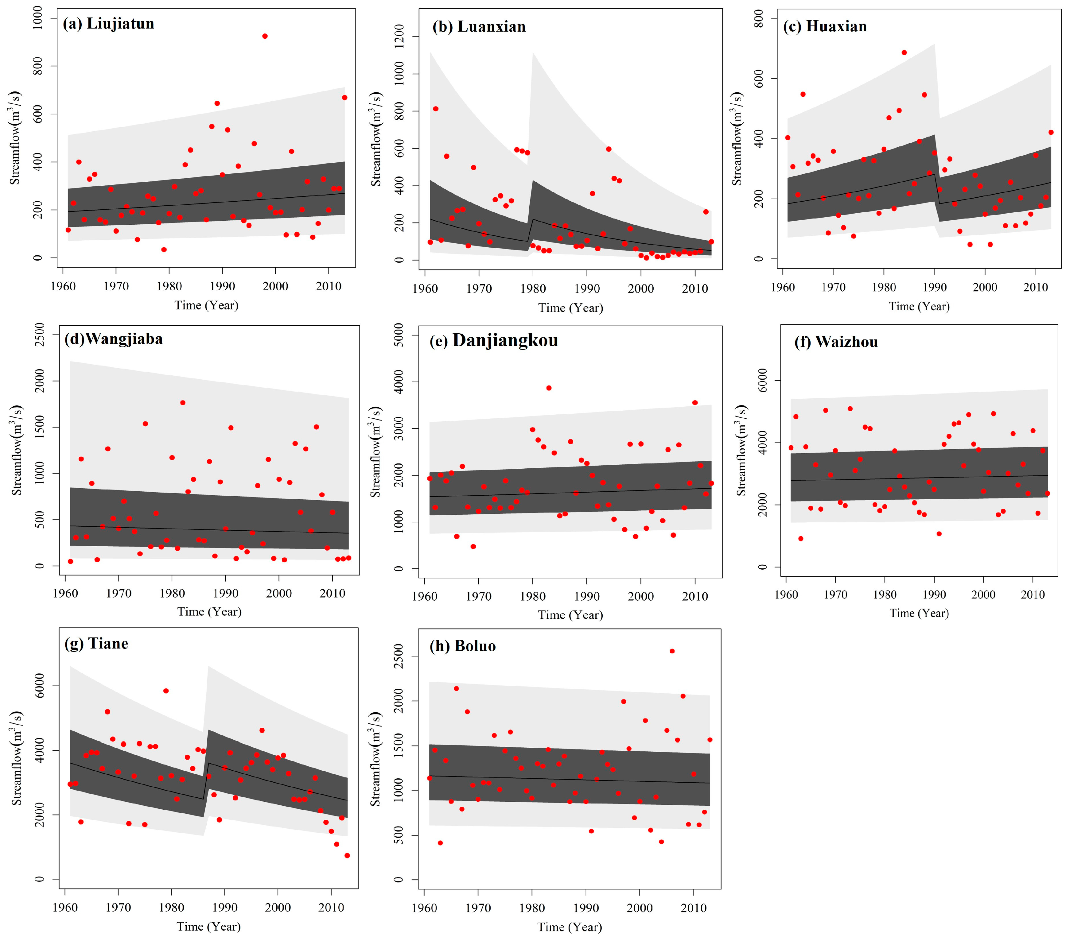
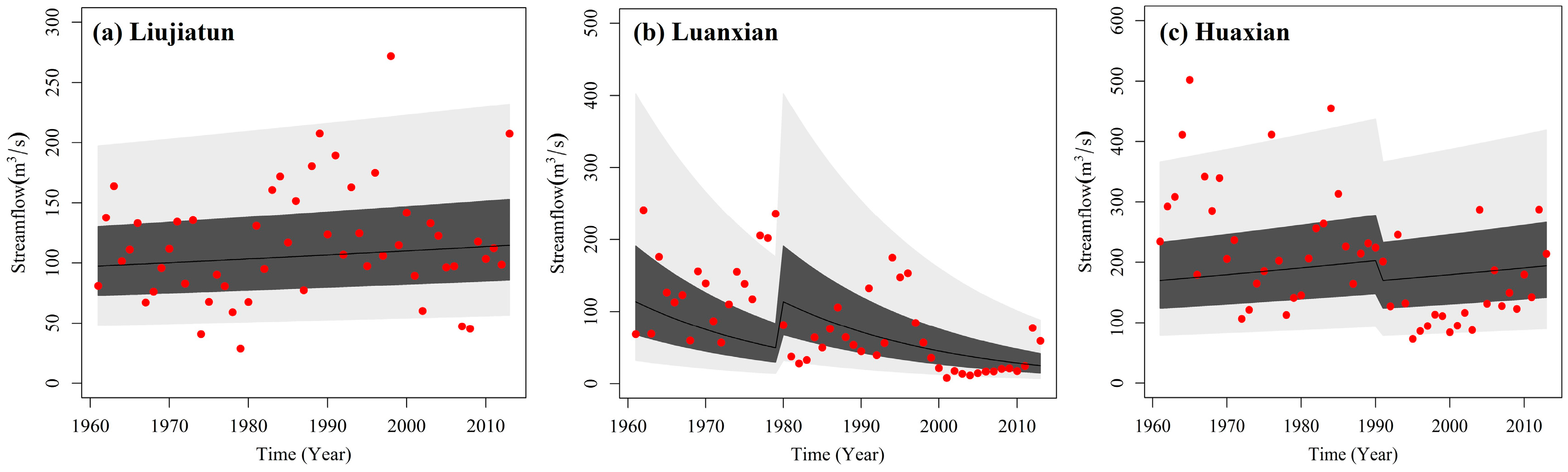
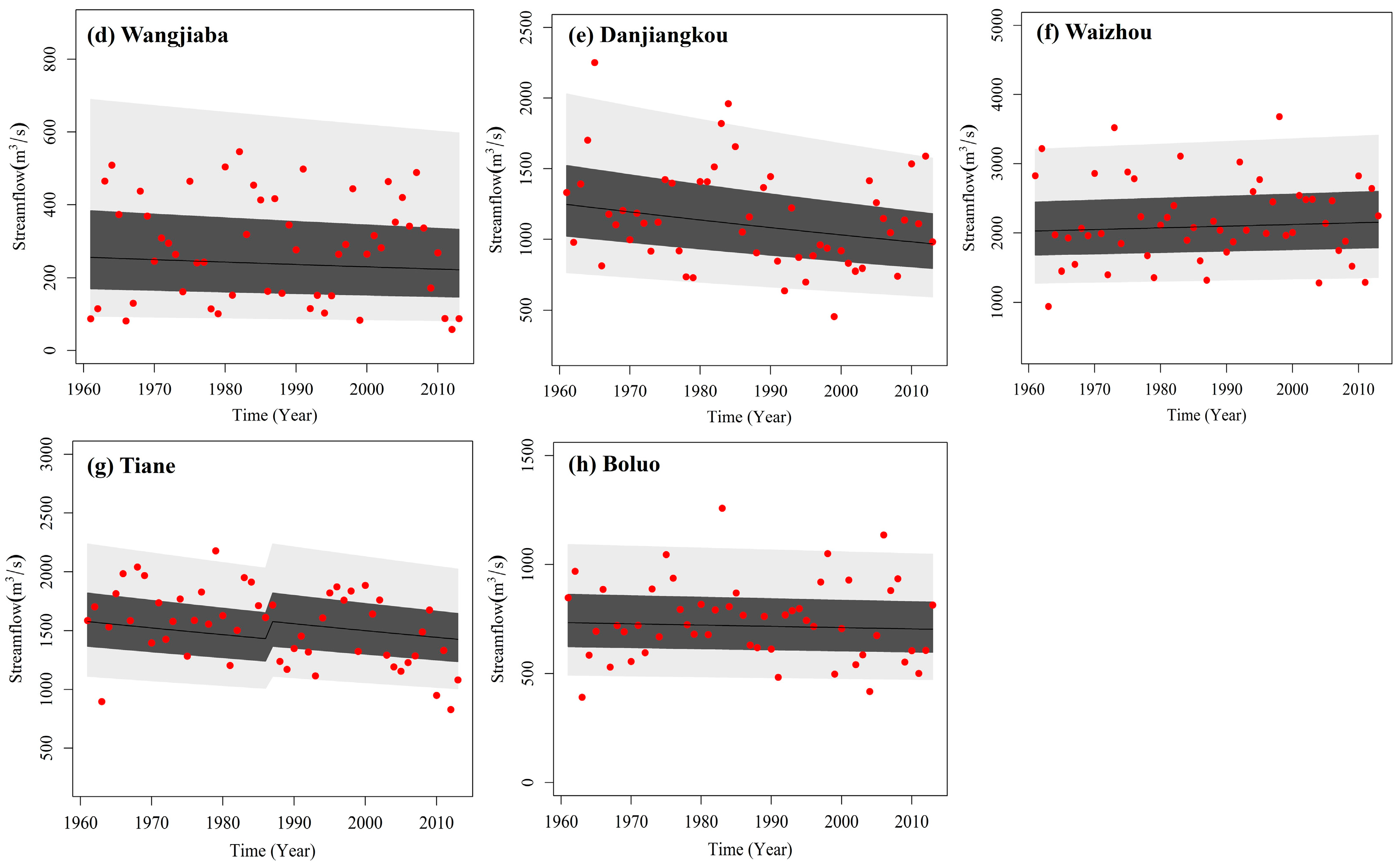
It can be seen from Table 5 that the nonstationarity models performed best for fitting the streamflow series at different time scales for the eight hydrological stations. At both 3-month and 12-month time scales, the gamma distribution was the optimal distribution for half of the selected stations (4 stations), followed by the lognormal and Weibull distribution. With respect to testing the stationarity, no models were found to be stationary with time-independent parameters (Table 5). Among the 16 selected models at different time scales, 12 models exhibited nonstationarity in (for mean), and 4 models exhibited nonstationarity in (for variance). No models of nonstationarity in mean and variance were selected. The statistic of (Table 5) also indicated that the selected nonstationarity model was an adequate fit for the streamflow series at different time scales at the respective stations. The averaged streamflow series in August was taken as an example to show the fitting of the GAMLSS model. Fitting of averaged streamflow series in August at different time scales for the eight stations using GAMLSS is shown in Figure 3 (3-month scale) and Figure 4 (12-month scale). The vast majority of the points were within the 0.05 and 0.95 quantiles (Figure 3 and Figure 4), indicating that the selected models were able to capture the variability of the data at both 3-month scale and 12-month scale. The centile curves of the GAMLSS modeling in eight stations exhibited temporal trend, showing that the fitted models captured non-linear behaviors associated with the streamflow series. For the three stations (Luanxian, Huaxian and Tiane) with change points, the 5% and 95% percentile curves were significantly impacted by the abrupt changes. Visual inspections of worm plots were also conducted to check the residuals. All the worm points were within the 95% confidence intervals (Figure 5 and Figure 6), indicating consistency between the selected nonstationarity model and the observed data at different time scales. Thus, the results indicated the GAMLSS-based modeling was able to capture the temporal variability of the streamflow series.
4.4. Construction of the SSIvar
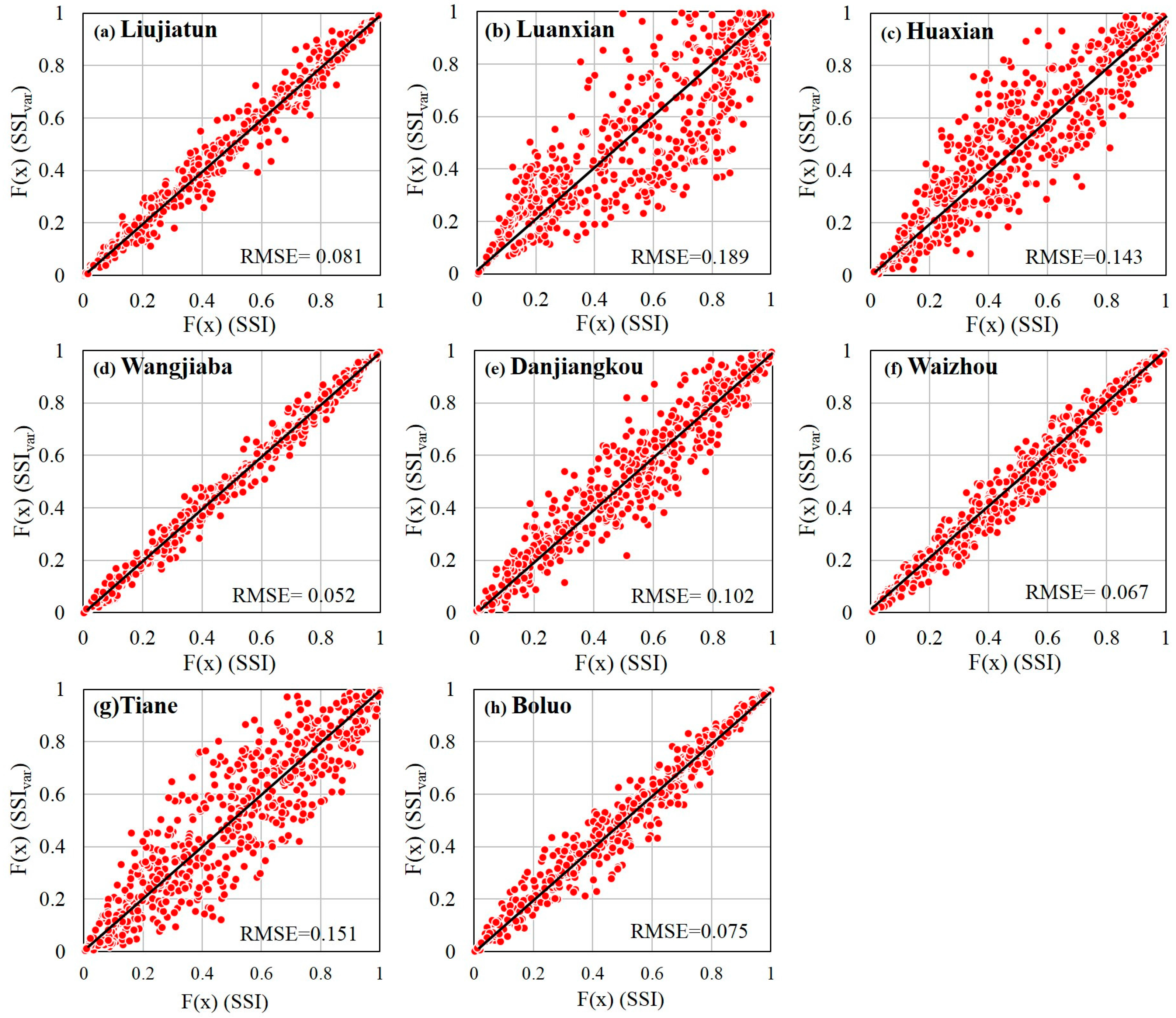
Based on the GAMLSS model, both the time-dependent SSI (SSIvar) and traditional SSI were employed to identify drought characteristics in the selected eight basins during 1961–2013. It can be seen from Figure 7 that noticeable differences existed in the values of cumulative probability F(x) for calculating SSI and SSIvar. The deviations of F(x) for SSI and SSIvar for different hydrological stations were varying in degree (Figure 7). Taking Luanxian and Wangjiaba stations as examples, the matching points were distributed around 1:1 line in Wangjiaba while the points were deviated from 1:1 line in Luanxian. The root mean square error (RMSE) of Luanxian (0.189) was larger than that in Wangjiaba (0.052). This may be because the streamflow series in Luanxian has change point and significant variation trend. During the procedure of SSI calculation, the cumulative probability F(x) was transformed to a standard normal deviation with a zero mean and unit variance, which is the value of SSI. Thus, the deviations of F(x) for calculating SSI and SSIvar could result in the differences between SSI and SSIvar.
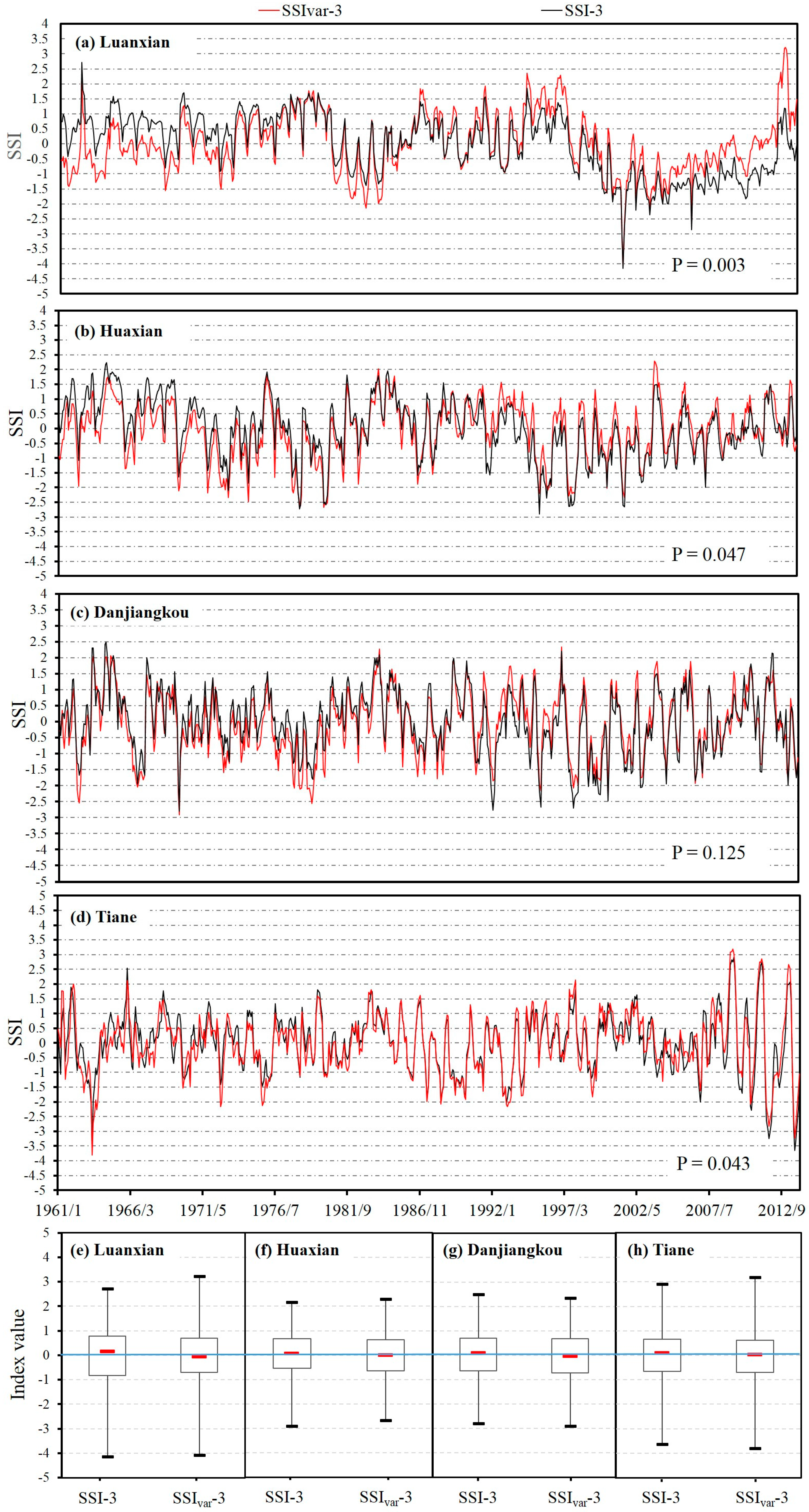
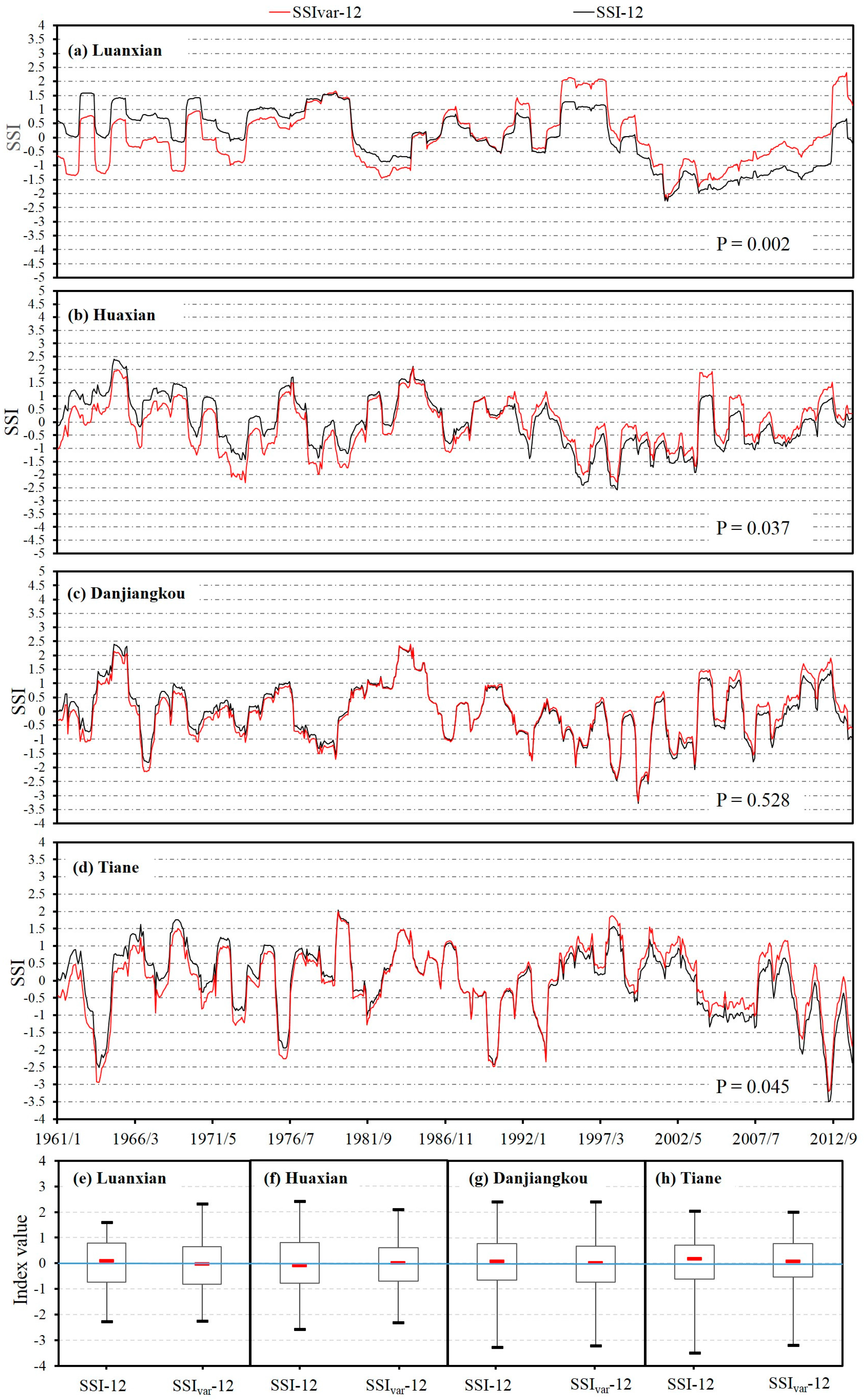
Taking Luanxian, Huaxian, Danjiangkou and Tiane as examples, to show the influence of change of parameter clearly, the SSIvar and traditional SSI during 1960–2013 in four basins are shown in Figure 8 (3-month scale) and Figure 9 (12-month scale). From Figure 8 and Figure 9, it can be seen that similar differences between SSI and SSIvar were observed in four basins at different time scales. For the selected basins, the drought severity shown by SSIvar was first more severe than traditional SSI, and then it was subsequently milder than traditional SSI. The stations with change points and significant trend changes (i.e., Luanxian, Huanxian and Tiane) have larger deviations between SSI and SSIvar than the other stations. For instance, for the basin above Luanxian station at 3-month scale (Figure 8a), obviously lower values were detected by SSIvar during 1961–1968 compared to traditional SSI, while notably higher values were found for SSIvar during 1992–2013. For the basin above Huaxian station at 12-month scale (Figure 9b), we can also observe that the values of SSI were higher than SSIvar during 1961–1990 (e.g., moderate drought was detected by SSIvar-12 in May 1972 (−1.43), while slight drought was characterized by SSI-12 (−0.76)), while being lower than SSIvar during 1991–2013. As the SSI is a standardized variate, the average values of the SSI and the standardized deviation must equal 0 and 1, respectively. Meanwhile, the two-sample Kolmogorov-Smirnov (KS) test [39] was used to test whether two indexes cons from same distribution. The KS test statistically showed that SSI and SSIvar are statistically different in Luanxian, Huaxian and Tiane stations at 95% confidence level (p < 0.05) (Figure 8 and Figure 9). It is worth noting that the boxplots of two SSI series show that the symmetry of the SSIvar is superior to that of the SSI at different time scales (Figure 8 and Figure 9), and it is closer to the standard normal distribution (zero mean and unit variance). Thus, compared to the traditional SSI, the SSIvar is capable of modeling the nonstationarity of streamflow series and is more appropriate for hydrological drought assessment within a changing environment.
5. Conclusions
In this study, streamflow series at eight different stations in the EAM region of China were modeled with nonstationarity distributions using GAMLSS. Based on the constructed nonstationarity distributions, the SSIvar was developed and used to estimate regional drought characteristics in the selected basin. The main conclusions can be summarized as follows:
- (1)
- Generalized Additive Models in Location, Scale and Shape (GAMLSS) provide a flexible and useful framework for modeling distributions of streamflow series considering both trend and change point. In particular, they provide the capability for modeling the non-stationarities in streamflow records.
- (2)
- Based on the selected optimal distribution, the developed SSIvar is capable of taking the nonstationarity of streamflow series into account; thus, it is likely to be more reliable and suitable than the traditional SSI for drought assessment in a changing environment. The differences between the SSIvar and SSI indicate that the presence of nonstationarity should be considered in regional drought assessment. The SSIvar is proven to be a feasible alternative for drought forecast and water resource management under changing environment.
Acknowledgments
This study was supported by the National Key R&D Program of China (2017YFA0603702) and the National Natural Science Foundation of China (41701023 and 41571028). We are very grateful to the editor and three anonymous reviewers for their valuable comments and constructive suggestions that helped us to greatly improve the manuscript.
Author Contributions
The research presented here was carried out in collaboration between all authors. Lei Zou processed the data and carried out the statistical analysis of results; Jun Xia, Like Ning, Dunxian She and Chesheng Zhan provided many significant suggestions on the methodology and structure of the manuscript.
Conflicts of Interest
The authors declare no conflict of interest.
References
- Wilhite, D.A. Drought: A Global Assessment; Routledge: New York, NY, USA, 2000. [Google Scholar]
- Mishra, A.K.; Singh, V.P. A review of drought concepts. J. Hydrol. 2010, 391, 202–216. [Google Scholar] [CrossRef]
- Wen, L.; Rogers, K.; Ling, J.; Saintilan, N. The impacts of river regulation and water diversion on the hydrological drought characteristics in the lower murrumbidgee river, Australia. J. Hydrol. 2011, 405, 382–391. [Google Scholar] [CrossRef]
- Wilhite, D.A.; Glantz, M.H. Understanding: The Drought Phenomenon: The Role of Definitions. Water Int. 1985, 10, 111–120. [Google Scholar] [CrossRef]
- Van Loon, A.F.; Laaha, G. Hydrological drought severity explained by climate and catchment characteristics. J. Hydrol. 2015, 526, 3–14. [Google Scholar] [CrossRef]
- Nalbantis, I.; Tsakiris, G. Assessment of hydrological drought revisited. Water Resour. Manag. 2009, 23, 881–897. [Google Scholar] [CrossRef]
- Zhu, Y.; Wang, W.; Singh, V.P.; Liu, Y. Combined use of meteorological drought indices at multi-time scales for improving hydrological drought detection. Sci. Total Environ. 2016, 571, 1058–1068. [Google Scholar] [CrossRef] [PubMed]
- Doell, P.; Fiedler, K.; Zhang, J. Global-scale analysis of river flow alterations due to water withdrawals and reservoirs. Hydrol. Earth Syst. Sci. 2009, 13, 2413–2432. [Google Scholar] [CrossRef]
- Shukla, S.; Wood, A.W. Use of a standardized runoff index for characterizing hydrologic drought. Geophys. Res. Lett. 2008, 35. [Google Scholar] [CrossRef]
- McKee, T.B.; Doesken, N.J.; Kleist, J. The relationship of drought frequency and duration to time scales. In Proceedings of the 8th Conference on Applied Climatology, Anaheim, CA, USA, 17–22 January; 1993; pp. 179–184. [Google Scholar]
- Vicente-Serrano, S.M.; Lopez-Moreno, J.I.; Begueria, S.; Lorenzo-Lacruz, J.; Azorin-Molina, C.; Moran-Tejeda, E. Accurate computation of a streamflow drought index. J. Hydrol. Eng. 2012, 17, 318–332. [Google Scholar] [CrossRef]
- Villarini, G.; Serinaldi, F.; Smith, J.A.; Krajewski, W.F. On the stationarity of annual flood peaks in the continental united states during the 20th century. Water Resour. Res. 2009, 45. [Google Scholar] [CrossRef]
- Zhang, Q.; Gu, X.H.; Singh, V.P.; Xiao, M.Z.; Xu, C.Y. Stationarity of annual flood peaks during 1951–2010 in the pearl river basin, China. J. Hydrol. 2014, 519, 3263–3274. [Google Scholar] [CrossRef]
- Villarini, G.; James, A.S.; Napolitano, F. Nonstationarity modeling of a long record of rainfall and temperature over Rome. Adv. Water Resour. 2010, 33, 1256–1267. [Google Scholar] [CrossRef]
- Vicente-Serrano, S.M.; Lopez-Moreno, J.I. Nonstationarity influence of the North Atlantic Oscillation on European precipitation. J. Geophys. Res.-Atmos. 2008, 113. [Google Scholar] [CrossRef]
- Milly, P.C.D.; Betancourt, J.; Falkenmark, M.; Hirsch, R.M.; Kundzewicz, Z.W.; Lettenmaier, D.P.; Stouffer, R.J. Climate change—Stationarity is dead: Whither water management? Science 2008, 319, 573–574. [Google Scholar] [CrossRef] [PubMed]
- Chang, N.-B.; Vasquez, M.V.; Chen, C.-F.; Imen, S.; Mullon, L. Global nonlinear and nonstationarity climate change effects on regional precipitation and forest phenology in Panama, Central America. Hydrol. Processes 2015, 29, 339–355. [Google Scholar] [CrossRef]
- Coulibaly, P.; Baldwin, C.K. Nonstationarity hydrological time series forecasting using nonlinear dynamic methods. J. Hydrol. 2005, 307, 164–174. [Google Scholar] [CrossRef]
- Verdon, D.C.; Wyatt, A.M.; Kiem, A.S.; Franks, S.W. Multidecadal variability of rainfall and streamflow: Eastern Australia. Water Resour. Res. 2004, 40. [Google Scholar] [CrossRef]
- Xu, X.; Yang, D.; Yang, H.; Lei, H. Attribution analysis based on the budyko hypothesis for detecting the dominant cause of runoff decline in Haihe basin. J. Hydrol. 2014, 510, 530–540. [Google Scholar] [CrossRef]
- Ishak, E.H.; Rahman, A.; Westra, S.; Sharma, A.; Kuczera, G. Evaluating the nonstationarity of Australian annual maximum flood. J. Hydrol. 2013, 494, 134–145. [Google Scholar] [CrossRef]
- Russo, S.; Dosio, A.; Sterl, A.; Barbosa, P.; Vogt, J. Projection of occurrence of extreme dry-wet years and seasons in Europe with stationary and nonstationarity standardized precipitation indices. J. Geophys. Res. Atmos. 2013, 118, 7628–7639. [Google Scholar] [CrossRef]
- Wang, Y.; Li, J.; Feng, P.; Hu, R. A time-dependent drought index for nonstationarity precipitation series. Water Resour. Manag. 2015, 29, 5631–5647. [Google Scholar] [CrossRef]
- El Adlouni, S.; Ouarda, T.B.M.J.; Zhang, X.; Roy, R.; Bobee, B. Generalized maximum likelihood estimators for the nonstationarity generalized extreme value model. Water Resour. Res. 2007, 43. [Google Scholar] [CrossRef]
- Underwood, F.M. Describing long-term trends in precipitation using generalized additive models. J. Hydrol. 2009, 364, 285–297. [Google Scholar] [CrossRef]
- Rigby, R.A.; Stasinopoulos, D.M. Generalized additive models for location, scale and shape. J. R. Stat. Soc. Ser. C 2005, 54, 507–544. [Google Scholar] [CrossRef]
- Slater, L.J.; Villarini, G. Evaluating the drivers of seasonal streamflow in the US Midwest. Water 2017, 9, 695. [Google Scholar] [CrossRef]
- Abramowitz, M.; Stegun, I.A. Handbook of Mathematical Functions; Dover: New York, NY, USA, 1965. [Google Scholar]
- Pettitt, A.N. A Non-Parametric Approach to the Change-Point Problem. J. R. Stat. Soc. 1979, 28, 126–135. [Google Scholar] [CrossRef]
- Mann, H.B. Nonparametric tests against trend. Econometrica 1945, 13, 245–259. [Google Scholar] [CrossRef]
- Kendall, M.G. Rank Correlation Methods; Griffin: London, UK, 1975. [Google Scholar]
- Alan, D.Z.; Justin, S.; Edwin, P.M.; Bart, N.; Eric, F.W.; Dennis, P.L. Detection of intensification in global- and continental-scale hydrological cycles: Temporal scale of evaluation. J. Clim. 2003, 16, 535–547. [Google Scholar]
- Zhang, X.B.; Harvey, K.D.; Hogg, W.D.; Yuzyk, T.R. Trends in Canadian streamflow. Water Resour. Res. 2001, 37, 987–998. [Google Scholar] [CrossRef]
- Stasinopoulos, D.M.; Rigby, R.A. Generalized additive models for location scale and shape (GAMLSS) in R. J. Stat. Softw. 2007, 23. [Google Scholar] [CrossRef]
- Lopez, J.; Frances, F. Nonstationarity flood frequency analysis in continental Spanish rivers, using climate and reservoir indices as external covariates. Hydrol. Earth Syst. Sci. 2013, 17, 3189–3203. [Google Scholar] [CrossRef]
- Akaike, H. A new look at the statistical model identification. IEEE Trans. Automat. Control 1974, 19, 716–723. [Google Scholar] [CrossRef]
- Filliben, J.J. The probability plot correlation coefficient test for normality. Technometrics 1975, 17, 111–117. [Google Scholar] [CrossRef]
- Buuren, S.V.; Fredriks, M. Worm plot: A simple diagnostic device for modelling growth reference curves. Stat. Med. 2001, 20, 1259–1277. [Google Scholar] [CrossRef] [PubMed]
- Press, W.H.; Teukolsky, S.A.; Vetterling, W.T.; Flannery, B.P. Numerical Recipes in C: The Art of Scientific Computing, 2nd ed.; Cambridge University Press: Cambridge, UK, 1992. [Google Scholar]
Figure 1.
The study area in EAM region.

Figure 2.
Pettitt’s test for detecting a change in the mean of annual streamflow. Horizontal lines represent the significance (solid line represent 1% and dotted line represent 5%).
Figure 2.
Pettitt’s test for detecting a change in the mean of annual streamflow. Horizontal lines represent the significance (solid line represent 1% and dotted line represent 5%).

Figure 3.
Centile curve plots for assessing the performance of the optimal nonstationarity model using time as covariate at 3-month scale. The red points are the observed streamflow at 3-month scale in August. The black line is the 50% centile curve, the dark grey region is the area between the 25% and 75% centile curves, and the light grey region is the area between the 5% and 95% centile curves.

Figure 4.
Centile curve plots for assessing the performance of the optimal nonstationarity model using time as covariate at 12-month scale. The red points are the observed streamflow at a 12-month scale in August. The black line is the 50% centile curve, the dark grey region is the area between the 25% and 75% centile curves, and the light grey region is the area between the 5% and 95% centile curves.


Figure 5.
Worm plots for the residuals from the GAMLSS models for streamflow series as illustrated in Figure 3. For a good fit, the data points should be aligned, preferably along the red solid line, but within the 95% confidence intervals indicated by the two grey dashed line.
Figure 5.
Worm plots for the residuals from the GAMLSS models for streamflow series as illustrated in Figure 3. For a good fit, the data points should be aligned, preferably along the red solid line, but within the 95% confidence intervals indicated by the two grey dashed line.

Figure 6.
Worm plots for the residuals from the GAMLSS models for streamflow series as illustrated in Figure 4. For a good fit, the data points should be aligned, preferably along the red solid line, but within the 95% confidence intervals indicated by the two grey dashed line.
Figure 6.
Worm plots for the residuals from the GAMLSS models for streamflow series as illustrated in Figure 4. For a good fit, the data points should be aligned, preferably along the red solid line, but within the 95% confidence intervals indicated by the two grey dashed line.

Figure 7.
Comparison of the cumulative probability F(x) between SSI and time-dependent SSI (SSIvar) for eight hydrological stations during 1961–2013.
Figure 7.
Comparison of the cumulative probability F(x) between SSI and time-dependent SSI (SSIvar) for eight hydrological stations during 1961–2013.

Figure 8.
Comparison between SSI-3 and SSIvar-3 for selected hydrological stations during 1961–2013: (a) Luanxian; (b) Huaxian; (c) Danjiangkou; (d) Tiane. The P represents the p-value of the KS test.
Figure 8.
Comparison between SSI-3 and SSIvar-3 for selected hydrological stations during 1961–2013: (a) Luanxian; (b) Huaxian; (c) Danjiangkou; (d) Tiane. The P represents the p-value of the KS test.

Figure 9.
Comparison between SSI-12 and SSIvar-12 for selected hydrological stations during 1961–2013: (a) Luanxian; (b) Huaxian; (c) Danjiangkou; (d) Tiane. The p represents the p-value of the KS test.
Figure 9.
Comparison between SSI-12 and SSIvar-12 for selected hydrological stations during 1961–2013: (a) Luanxian; (b) Huaxian; (c) Danjiangkou; (d) Tiane. The p represents the p-value of the KS test.


Table 1.
Drought classifications based on the traditional SSI.
| State | Categories | SSI Values |
|---|---|---|
| D0 | Extreme Drought | (−∞, −2) |
| D1 | Severe Drought | [−2, −1.5) |
| D2 | Moderate Drought | [−1.5, −1] |
| D3 | Slight Drought | [−1, 0) |
| D4 | Normal | [0, +∞) |
Table 2.
Summary of the distributions used to model the streamflow series at different time scales in our study.
Table 2.
Summary of the distributions used to model the streamflow series at different time scales in our study.
| Distribution | Probability Density Function | Distribution Moments | Link Functions |
|---|---|---|---|
| Gamma | |||
| Lognormal | |||
| Gumbel | |||
| Weibull | |||
| Logistic |
Table 3.
Information on the hydrological stations considered in this study.
| River Basin | Station | Drainage Area (km2) | Longitude | Latitude | Climatic Zone | Mean (m3/s) |
|---|---|---|---|---|---|---|
| SHRB | Liujiatun (LJT) | 19,665 | 125.08 | 49.25 | Humid and semi-humid | 115.09 |
| HRB | Luanxian (LX) | 44,100 | 118.75 | 39.73 | Semi-arid and semi-humid | 83.73 |
| YRB | Huaxian (HX) | 106,498 | 109.76 | 34.58 | Arid and semi-arid | 204.90 |
| HURB | Wangjiaba (WJB) | 30,630 | 115.60 | 32.43 | Humid and semi-humid | 282.62 |
| YARB | Danjiangkou (DJK) | 159,000 | 111.51 | 32.58 | Humid | 1141.64 |
| Waizhou (WZ) | 80,948 | 115.84 | 28.63 | Humid | 2164.33 | |
| PRB | Tiane (TE) | 105,535 | 107.16 | 24.99 | Humid | 1528.32 |
| Boluo (BL) | 25,325 | 114.30 | 23.17 | Humid | 737.71 |
Table 4.
Results of analysis of trends in streamflow series for the eight hydrological stations at an annual scale.
Table 4.
Results of analysis of trends in streamflow series for the eight hydrological stations at an annual scale.
| Stations | MK | |
|---|---|---|
| Liujiatun (LJT) | 0.198 | 0.142 |
| Luanxian (LX) | 0.475 | −2.352 |
| Huaxian (HX) | 0.397 | −1.992 |
| Wangjiaba (WJB) | −0.137 | −0.691 |
| Danjiangkou (DJK) | 0.272 | −1.155 |
| Waizhou (WZ) | −0.073 | 0.093 |
| Tiane (TE) | 0.202 | −2.553 |
| Boluo (BL) | 0.066 | −0.351 |
Note: MK denotes Mann-Kendall trend. The bold values denote significant trends at 95% confidence level.
Table 5.
Summary of results for the GAMLSS models of eight hydrological stations in EAM region (the critical values of the Filliben correlation coefficient is and the bigger than , indicating that the nonstationarity model passes the goodness-of-fit test).
Table 5.
Summary of results for the GAMLSS models of eight hydrological stations in EAM region (the critical values of the Filliben correlation coefficient is and the bigger than , indicating that the nonstationarity model passes the goodness-of-fit test).
| Stations | Optimal CDF | Stationary | Nonstationarity in (Mean) | Nonstationarity in (Variance) | Nonstationarity in both and |
|---|---|---|---|---|---|
| Monthly averaged AIC values and for stationary and optimal nonstationarity models (3-month scale) AIC/ | |||||
| Liujiatun (LJT) | LOGNO | 506.34/0.988 | 503.17/0.991 (Y) | — | — |
| Luanxian (LX) | WEI | 530.36/0.981 | 509.67/0.986 (Y) | — | — |
| Huaxian (HX) | GA | 636.00/0.985 | 627.37/0.989 (Y) | — | — |
| Wangjiaba (WJB) | GA | 676.77/0.980 | 675.63/0.981 (Y) | — | — |
| Danjiangkou (DJK) | GA | 783.77/0.992 | 780.92/0.994 (Y) | — | — |
| Waizhou (WZ) | LOGNO | 853.29/0.982 | 849.13/0.983 (Y) | — | — |
| Tiane (TE) | GA | 796.66/0.983 | 787.23/0.985 (Y) | — | — |
| Boluo (BL) | LOGNO | 727.17/0.991 | — | 725.74/0.992 (Y) | — |
| Monthly averaged AIC values for stationary and optimal nonstationarity models (12-month scale) AIC/ | |||||
| Liujiatun (LJT) | GA | 558.34/0.992 | 553.36/0.993 (Y) | — | — |
| Luanxian (LX) | GA | 573.77/0.983 | 553.55/0.983 (Y) | — | — |
| Huaxian (HX) | LOGNO | 632.70/0.982 | 622.24/0.983 (Y) | — | — |
| Wangjiaba (WJB) | WEI | 683.71/0.975 | — | 680.13/0.979 (Y) | — |
| Danjiangkou (DJK) | LOGNO | 781.23/0.989 | 778.44/0.991 (Y) | — | — |
| Waizhou (WZ) | GA | 828.92/0.991 | — | 825.65/0.993 (Y) | — |
| Tiane (TE) | WEI | 770.24/0.985 | 763.67/0.988 (Y) | — | — |
| Boluo (BL) | GA | 707.72/0.987 | — | 702.34/0.991 (Y) | — |
© 2018 by the authors. Licensee MDPI, Basel, Switzerland. This article is an open access article distributed under the terms and conditions of the Creative Commons Attribution (CC BY) license (http://creativecommons.org/licenses/by/4.0/).
Share and Cite
MDPI and ACS Style
Zou, L.; Xia, J.; Ning, L.; She, D.; Zhan, C. Identification of Hydrological Drought in Eastern China Using a Time-Dependent Drought Index. Water 2018, 10, 315. https://doi.org/10.3390/w10030315
AMA Style
Zou L, Xia J, Ning L, She D, Zhan C. Identification of Hydrological Drought in Eastern China Using a Time-Dependent Drought Index. Water. 2018; 10(3):315. https://doi.org/10.3390/w10030315
Chicago/Turabian StyleZou, Lei, Jun Xia, Like Ning, Dunxian She, and Chesheng Zhan. 2018. "Identification of Hydrological Drought in Eastern China Using a Time-Dependent Drought Index" Water 10, no. 3: 315. https://doi.org/10.3390/w10030315
Note that from the first issue of 2016, this journal uses article numbers instead of page numbers. See further details here.