Using Sap Flow Data to Parameterize the Feddes Water Stress Model for Norway Spruce


1
Department of Geography, University of Bonn, Meckenheimer Allee 166, 53115 Bonn, Germany
2
Agrosphere Institute (IBG-3), Forschungszentrum Jülich, Wilhelm-Johnen-Straße, 52428 Jülich, Germany
3
Dendro-Labor Windeck, Tree-Ring-Analyses, 51570 Windeck, Germany
*
Author to whom correspondence should be addressed.
Water 2018, 10(3), 279; https://doi.org/10.3390/w10030279
Submission received: 8 December 2017
/
Revised: 20 February 2018
/
Accepted: 5 March 2018
/
Published: 7 March 2018
(This article belongs to the Special Issue Soil-Plant-Water Relationships )
Abstract
:Tree water use is a key variable in forest eco-hydrological studies and is often monitored by sap flow measurements. Upscaling these point measurements to the stand or catchment level, however, is still challenging. Due to the spatio-temporal heterogeneity of stand structure and soil water supply, extensive measuring campaigns are needed to determine stand water use from sap flow measurements alone. Therefore, many researchers apply water balance models to estimate stand transpiration. To account for the effects of limited soil water supply on stand transpiration, models commonly refer to plant water stress functions, which have rarely been parameterized for forest trees. The aim of this study was to parameterize the Feddes water stress model for Norway spruce (Picea abies [L.] Karst.). After successful calibration and validation of the soil hydrological model HYDRUS-1D, we combined root-zone water potential simulations with a new plant water stress factor derived from sap flow measurements at two plots of contrasting soil moisture regimes. By calibrating HYDRUS-1D against our sap flow data, we determined the critical limits of soil water supply. Drought stress reduced the transpiration activity of mature Norway spruce at root-zone pressure heads <−4100 cm, while aeration stress was not observed. Using the recalibrated Feddes parameters in HYDRUS-1D also improved our water balance simulations. We conclude that the consideration of sap flow information in soil hydrological modeling is a promising way towards more realistic water balance simulations in forest ecosystems.
1. Introduction
Tree water use is a key variable in forest eco-hydrological studies and closely linked to meteorological conditions and soil water availability [1,2,3,4]. To monitor the water use of individual trees, a number of methods are available [5,6]. Sap flow measurements are most popular, not only because they are cost-efficient and easy to apply. They also yield reasonable information on temporal transpiration patterns and deliver valuable insights into plant-physiological responses to varying hydro-climatic conditions (e.g., soil moisture limitations). Respectively, [7] identified sap flow as a “key trait in the understanding of plant hydraulic functioning”.
However, to make stem-based sap flow measurements valuable for watershed and land use managers, they need to be scaled to a ground area basis [2]. Common scalars in this regard are sapwood area, basal area, diameter or circumference at breast height and leaf area [2,8,9]. However, the scaling of sap flow measurements from the tree to the forest stand includes many uncertainties. To begin with, different measuring approaches yield differing estimates of sap flow rates per tree [9,10,11,12]. This is partly related to uncertainties in signal transformation [13,14,15], but also to radial and circumferential variations in sap flow density, which complicates the scaling from the point measurement to water use by tree [16,17,18,19,20,21]. Furthermore, sap flow activity and trans-sectional sapwood distribution vary with tree age, tree dimensions, social position of the tree and also with soil water supply [4,22,23,24,25]. Thus, extensive measurement campaigns are needed to get a solid estimate of stand water use from sap flow measurements alone.
Alternatively, water balance models can be used to estimate stand transpiration. Such models basically calculate transpiration as a function of atmospheric boundary conditions (potential evapotranspiration), soil water supply and vegetation characteristics from which leaf area index (LAI) and stomatal conductance are the most important [2,26]. Under non-limiting conditions, transpiration generally follows the dynamic of atmospheric demand. However, the response of plants to variabilities in soil water supply is highly species specific. To account for these species-specific feedbacks in the soil-vegetation-atmosphere system, water balance models commonly include plant water stress functions (e.g., [27,28]), where critical limits of soil water supply can be adapted according to the vegetation characteristics. For many agricultural crops, such thresholds have already been defined and included into models that help to optimize irrigation scheduling and crop yields [3]. However, little is known about the species-specific water-stress-response of forest trees. Since forests play an important role in regional and trans-regional water cycles, there is evidence that an improved knowledge of tree species specific water stress thresholds would greatly enhance the simulations of water fluxes from the forest stand to the watershed and landscape scale [2,9,29,30,31].
The aim of this study was: (1) to parameterize the Feddes water stress model for Norway spruce, which is a wide-spread and economically important species in Europe; (2) to investigate if the species-specific calibration of the Feddes parameters can improve water balance simulations in the soil hydrological model HYDRUS-1D [32]. In a first step, we used HYDRUS-1D to estimate the root zone water potential for two research plots with contrasting soil water regimes. We derived the Feddes parameters for Norway spruce from correlations of the simulated water potentials and a new sap flow-based plant water stress factor.
2. Materials and Methods
2.1. Study Area
The study was conducted in the 27 ha Wüstebach experimental test site [33], which is located in the Rur River catchment close to the German-Belgian border (Figure 1). The test site belongs to the TERENO Eifel/Lower Rhine Valley Observatory [34,35]. Altitudes range from 595 m a.s.l. in the north to 628 m a.s.l. in the south. While hillslopes are dominated by shallow Cambisols and Planosols, Gleysols and Histosols have developed in the groundwater-influenced riparian zone along the Wüstebach stream. The soils mainly show a silty clay loam texture with a medium to high coarse material fraction and a litter layer on top [36]. The soils in the valley bottom have slightly higher bulk densities and lower (macro-) porosities and skeleton contents than those on the hillslopes [36,37,38]. The climate is characterized by an annual mean temperature of 7 °C [39] and a mean annual precipitation of 1220 mm [33]. The annual potential evapotranspiration of the years 2010–2013 was 630 mm [40]. The catchment is forested with Norway spruce that were planted in the late 1940s [41]. The trees have now reached a height of about 28 m and the tree density is about 320 trees ha−1.
2.2. Data and Experimental Design
We used sap flow data from two research plots (Figure 1) from which one (Riparian) is located in the wetter valley bottom (~600 m a.s.l.), while the other is situated on the drier hillslope (Slope see Figure 1) at ~610 m a.s.l. With a gradient of 2°, the Riparian plot is slightly inclined towards N, while the Slope plot shows a gradient of 8° in NNW direction. Prevailing soil types are Gleysol (Riparian) and Cambisol/Planosol (Slope).
At each plot, sap flow of four trees was monitored over 2 years (2009–2010) using improved Granier-type sap flow sensors (SF-L 20/33, Ecomatik, Dachau, Germany). The classic Granier system consists of two sensor probes inserted radially into the sapwood, one above the other. The upper probe is equipped with a heating element and a thermocouple, thus recording the heat dissipation due to sap flow. The lower probe measures the ambient reference temperature of the wood. Our improved sensor version includes another pair of thermocouples that is placed horizontally to the upper heated probe to account for natural inner-wood temperature variations. The mean of the inner-wood temperature variations recorded by these additional reference probes is subtracted from the values recorded by the classic Granier system before applying the Granier formula, where sap flux density is derived from the temperature gradient between the heated and the lower reference probe using the empirical equation [42,43]:
in which SFD is the sap flux density (g·m−2·s−1), ∆T is the actual temperature gradient between the two probes and ∆Tmax the maximum temperature gradient measured between the probes in a given time period. Following [15], who found a daily ∆Tmax determination suitable for the study area, we determined ∆Tmax on the basis of a 24 h moving window (12 h before and 12 h after the actual point of measurement). This dynamic ∆Tmax determination procedure appeared the best opportunity to handle potential drifts in ∆Tmax.
The sap flow sensors were installed in the outermost 3.3 cm of the sapwood on the north side of the sample trees at ~1.5 m above ground. To ensure that the sensor probes were completely surrounded by sapwood (i.e., no heartwood), we determined each tree’s sapwood depth by drill hole analyses before installing the sap flow sensors. We insulated our probes with reflective polystyrene and plastic boxes. The temperature gradients measured and recorded at a datalogger (type CR1000, Campbell Scientific Ltd., Logan, UT, USA) in 30-min time steps.
Data gaps were filled using a simple three step procedure: (1) linear regression among all sap flow series within one plot; (2) choice of the data series with the highest coefficient of determination (R²) with the data series to be gap-filled; (3) interpolation of missing values from the respective regression line. Mean daily sap flow density was calculated from the gap-filled hourly data
Soil moisture was monitored by the wireless sensor network SoilNet, which provides catchment-wide information on soil water dynamics in 5, 20 and 50 cm depths at 150 measuring locations (see Figure 1). The installed measuring devices are the capacitance soil water content sensors ECH2O EC-5 and ECH2O 5TE (Decagon Devices, Pullman, WA, USA) [44]. Sensor calibration was performed according to [37]. For this study, we used the mean daily soil moisture at 20 and 50 cm depth of two SoilNet stations located close to our sap flow plots (Figure 1). Although there are other SoilNet stations closer to the Slope plot than the chosen station SN 28, we used this station, because it is located at the same elevation as the sap flow plot. The SoilNet data from 5 cm depth was not considered in this study, because the respective sensors were located in the litter layer and not in the mineral soil we focus on (Figure 2).
Grass reference evapotranspiration ET0 was calculated using the FAO-Penman-Monteith method [45] following [40], who first calculated hourly ET0 values and then aggregated these to daily sums. The required input data were obtained from the TERENO weather station Schöneseiffen (3.4 km east of the Wüstebach site). For gap-filling, linear regression predictors from the same variables of the TERENO station Selhausen (40 km north) were used. To calculate potential evapotranspiration for specific crops (not grass), ET0 is usually multiplied with the crop coefficient Kc. However, according to [45] a Kc value of 1 can be used for coniferous forests. Therefore, we assume ET0 to represent potential forest transpiration in this study. Daily precipitation was obtained from the Kalterherberg weather station of the German Meteorological Service (DWD), which is located 9.6 km east from of the test site and representative for our study site [46]. The precipitation data were corrected for systematic measurement errors according to [47].
The mean leaf area index was determined by averaging respective measurements (SunScan SS1, Delta-T Devices Ltd., Cambridge, UK) at 60 selected SoilNet locations within the Wüstebach site.
2.3. Estimating Root-Zone Water Potential
The water potential of the root-zone is a measure for the energy needed to extract water from the soil [48]. Therefore, we consider the root-zone water potential to be a solid measure to characterize the water availability for plants. However, since water potential is not measured at the SoilNet stations, we used the 1-D Richards equation as implemented in the HYDRUS-1D software [32] to inversely determine water potential dynamics from the soil water content (SWC) observations. This is a common approach in soil hydrology, which also allows for the integration of the point scale SWC measurements into vertical soil moisture profiles. In HYDRUS-1D the soil hydraulic properties are parameterized with the Mualem-van Genuchten model [49]:
where
where h is the pressure head (cm), θr is the residual water content (cm³ cm−3), θs the saturated water content (cm³ cm−3), α and n are empirical parameters, from which α is related to the air-entry pressure value and n is related to the pore size distribution, m is the retention curve shape parameter, which is dependent on n, Ks is the saturated hydraulic conductivity (cm h−1), and Se is the relative soil saturation.
Both research plots were modelled separately and in daily time steps. As top boundary conditions, we used the corrected precipitation data and the gap-filled potential evapotranspiration data (see above). The latter was divided into potential evaporation (E0) and potential transpiration (T0) on the basis of the leaf area index (LAI) [45]. In this study, mean LAI on site was 4.8 (with a standard deviation of 0.7) and assumed to be constant in time. Therefore, the differentiation between E0 and T0 was of minor importance. However, applying our approach to deciduous trees with seasonal LAI dynamics would require the consideration of the T0 limitation by LAI. For the hillslope plot (Slope) we set the lower boundary condition to free drainage, following [50], who found this option to provide the best HYDRUS-1D simulation results for the Wüstebach catchment.
To account for the groundwater fluctuations in the riparian zone, the lower boundary condition for the wetter plot (Riparian) was set to deep drainage [51]. For the deep drainage option, the discharge rate at the bottom of the soil profile is defined as a function of the position of the groundwater table and the empirical parameters Aqh and Bqh [52]:
in which q(h) (cm day−1) is the discharge rate, h (cm) is the pressure head at the bottom of the soil profile, Aqh (cm day−1) and Bqh (cm−1) are empirical parameters and GWLref (cm) is the reference groundwater depth. We manually optimized Aqh and Bqh with regard to the best fit (root-mean-square error) between measured and simulated soil moisture dynamics.
Depending on the local site conditions [36,38] we discretized the HYDRUS-1D soil profiles into two (Riparian) and three (Slope) materials (one/two soil horizons plus an organic litter layer on top) (Figure 2). The hydraulic properties of the litter layer were parameterized according to [53]. For the other soil materials, we inversely estimated the Mualem-van-Genuchten parameters from our measured SWC in 20 and 50 cm depth. We therefore used the inverse solution option as implemented in HYDRUS-1D, where the objective function Φ is minimized applying the Levenberg-Marquardt nonlinear least-squares fitting approach (for detailed information on the optimization procedure, see [32]).
Root water uptake in HYDRUS-1D depends on the root distribution over the soil depth and on soil water availability [32]. For our Norway spruce plots, we assumed a rooting depth of 45 cm, which is in line with [54,55]. The root zone was assumed to start below the litter layer, which had a thickness of 6 (Slope) and 9 cm (Riparian), respectively (Figure 2). The root density in spruce forests is typically highest in the upper soil layers [56,57,58]. Therefore, we assumed the potential root water uptake factor to be 1 in the uppermost 15 cm of the mineral soil (one third of the root zone). For the deeper layers, we implemented a linear decrease of the potential root water uptake factor from 1 in 15 cm depth to 0 in 45 cm depth.
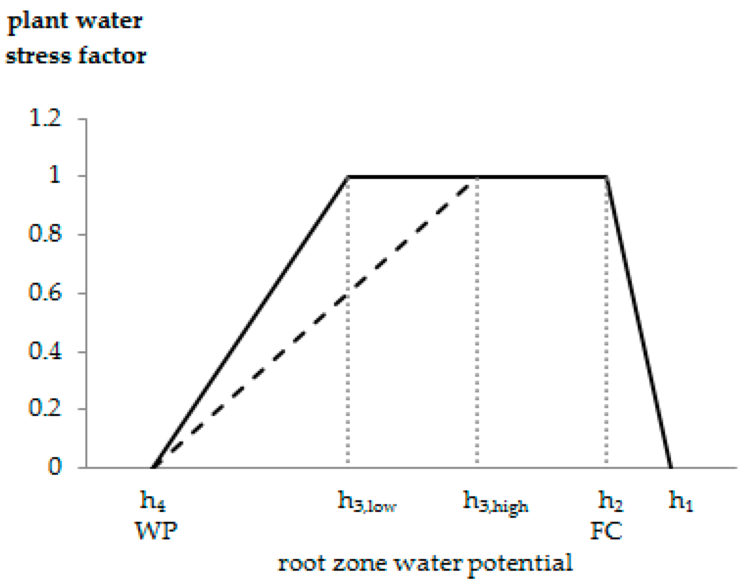
To account for reduced water uptake rates in case of water stress (aeration stress and drought stress), we used the Feddes plant water stress function [28] as implemented in HYDRUS-1D. In the Feddes function, a dimensionless water stress factor represents the water stress level of the plant as a function of the root zone water potential (Figure 3). This water stress factor corresponds to the ratio of actual (Tact) and potential (maximum possible) transpiration (T0) and thus ranges from 0 (maximum stress/no root water uptake) to 1 (no stress/optimum root water uptake). Optimum root water uptake (T0 = Tact) is given between h2 (field capacity FC) and h3 (onset of drought stress). The decreasing plant water stress between h2 and h1 considers that plants typically experience increasing aeration stress towards saturated conditions; h4 corresponds to the permanent wilting point (WP), h1 to the point of maximum aeration stress (anoxic conditions).
Presuming that h3 decreases with decreasing T0, HYDRUS-1D allows for making h3 a function of T0. The range of T0, within which h3 becomes a function of T0 may be defined by the user, but is usually 1–5 mm day−1 (default values). The h3 value for T0 < 1 mm day−1 is called h3,low, that for T0 > 5 mm day−1 h3,high. If T0 is between 1 and 5 mm day−1 and the soil dries out to less than h3,high, the critical root-zone water potential, at which potential root water uptake is reduced to the actual root water uptake, is linearly related to T0 [32].
As start values for the model inversion, we used the Feddes parameters (in cm pressure head) as proposed by [59] for a 90-years-old spruce site in the Czech Republic, where h1 = h2 = 0 cm, h3,high = −600 cm, h3,low = −1200 cm, and h4 = −15,000 cm. Later, we manually optimized the Feddes parameters on the basis of our sap flow data (see below).
2.4. Model Validation
We validated our model setup on the basis of the soil moisture measurements in 20 and 50 cm depth using a split-sample approach. To consider the observed drop in soil moisture between the years 2010 and 2011 in the optimization procedure, we chose the years 2009–2011 as the calibration period. For validation, we used another three year period (2012–2014). The goodness-of-fit between observed and simulated data was assessed on the basis of the root mean squared error (RMSE). Our sap flow data was restricted to the years 2009 and 2010 and was therefore not considered for model validation.
2.5. Parameterizing the Feddes Model Using Sap Flow Data
In the classical Feddes approach, plant water stress is derived from the ratio of Tact and T0 (see above). The assumption is that this ratio is mainly dependent on soil water supply. However, [60] showed that Norway spruce reacts to high midday vapor pressure deficits (VPD) by closing stomata. Thus, the trees physiologically reduce their own transpiration activity on many days of the growing season. In order not to mix-up this atmospheric stress reaction with actual soil water stress, we applied a new approach to calculate plant water stress from our sap flow data. This approach was based on the assumption that the micro-climate is identical at both plots; thus, in case of atmospheric stress, all trees (Riparian and Slope plot) show the same physiological reaction.
For each tree we determined the 6 highest SFD values per day. We averaged these maxima by day and plot and normalized the resulting data series (SFDn,rip for Riparian and SFDn,sl for Slope).
For the Riparian plot, we assumed optimum soil water supply, because due to the constant influence of groundwater the soil at this plot showed relatively high soil water contents throughout the study period and critical levels of soil water supply as reported from other studies [23,24,31,61,62] were never reached. We calculated a drought stress factor SFDdrought (1: optimum water supply; 0: maximum water stress) for the Slope plot by dividing SFDn,sl by SFDn,rip. To ensure that potential aeration stress at the Riparian plot would not affect our drought stress function, we only used data of dry days (3rd day without precipitation). We plotted SFDdrought against the simulated Slope water potential and analyzed the correlation between SFDdrought and root zone h for different levels of soil water shortage. The data which showed the highest significant correlation (R² and Student’s t-test) between SFDdrought and root zone h was used to determine the drought-stress trendline. The intersection of this trendline with the x-axis corresponds to the simulated Slope root zone water potential at maximum drought stress (SFDdrought = 0) and was therefore interpreted as the permanent wilting point h4.
During model calibration we found that the parameter h3,high was independent from mean daily sap flow dynamics and hence could not be optimized using sap flow measurements. However, it is well-known that at high levels of atmospheric demand, the transpiration rate of spruce forests decreases with increasing vapor pressure deficit [23]. This was also confirmed by our own sap flow measurements (data not shown). While coupled soil–plant–atmosphere continuum models are able to account for atmospheric stress, this process is not implemented in HYDRUS-1D. Nevertheless, since the Feddes approach is differentiated into h3,high and h3,low, atmospheric stress can be considered by adapting the T0 range at which h3 is a function of T0. The study of [60] suggests that spruce trees reduce transpiration when midday vapor pressure deficit exceeds 1250 Pa independent of soil wetness. Accordingly, we analyzed days with maximum VPD of approx. 1250 Pa and found that a T0 value of 2.7 mm day−1 can be used as lower boundary for the h3-dependent T0 range. Furthermore, we used T0 at the day of maximum observed daily SFD (4.8 mm day−1) as the upper boundary for the h3-dependent T0 range.
To detect potential aeration stress at the Riparian plot, we selected days, for which no drought stress was observed on the Slope plot. For these days, SFDn,sl was used as a reference for optimum water supply. We calculated an aeration stress factor SFDaeration (1: optimum water supply; 0: maximum water stress) by dividing SFDn,rip by SFDn,sl. To determine the Feddes parameters h1 and h2, we plotted SFDaeration against the simulated Riparian root-zone water potential and analyzed the observed data trend as described for SFDdrought.
2.6. Relative Extractable Soil Water (REW)
It is well known that absolute soil water contents do not fully reflect the actual soil water status [29,63]. Therefore, many researchers refer to the relative extractable soil water (REW) as a measure of soil water status (e.g., [4,23,63,64,65,66]). To compare our Feddes parameters with critical REW values from the literature, we calculated the mean root-zone water contents corresponding to the reported critical REW according to the relations described by [64,66]:
in which θ is the actual water content, θFC is the water content at field capacity, and θPWP is the water content at permanent wilting point. To be consistent with the literature [64,66], we chose θ at −300 cm pressure head (−0.03 MPa) for θFC and θ at −16,300 cm pressure head (−1.6 MPa) for θPWP.
2.7. Uncertainty Assessment
To assess the uncertainty of the simulated root zone water potential related to the assumed rooting depth and the shape of the potential root water uptake function, we performed a sensitivity analysis.
First, we ran the model for each plot assuming constant rooting depth (45 cm), but differing root distributions (factor 1 in the uppermost 15/30/45 cm of the mineral soil and linear decrease from 1 to 0 towards the bottom of the root zone). Then, we varied the rooting depth (30/40/50/60 cm) and simulated the respective root zone water potentials assuming a root distribution factor of 1 for the uppermost 15 cm of the mineral soil linearly decreasing from 1 to 0 between 15 cm depth and the final rooting depth.
Test statistics (Mann-Whitney U-test) on the similarity of the simulated root zone water potentials were conducted on the log scale.
To evaluate the small-scale variability of soil water supply around the sap flow stations and to ensure that the selected SoilNet measuring locations are representative for our sap flow plots, we simulated the root zone water potentials of 4 (Riparian) and 7 (Slope) surrounding SoilNet locations (Figure 1). These simulations were again performed on the basis of calibrated and validated Mualem-van Genuchten parameters.
From the average root zone water potentials of the surrounding SoilNet locations, we determined the Feddes parameters as described before and compared the results with the water stress thresholds as resulting from the initial research setup.
3. Results
3.1. Sap Flow Data
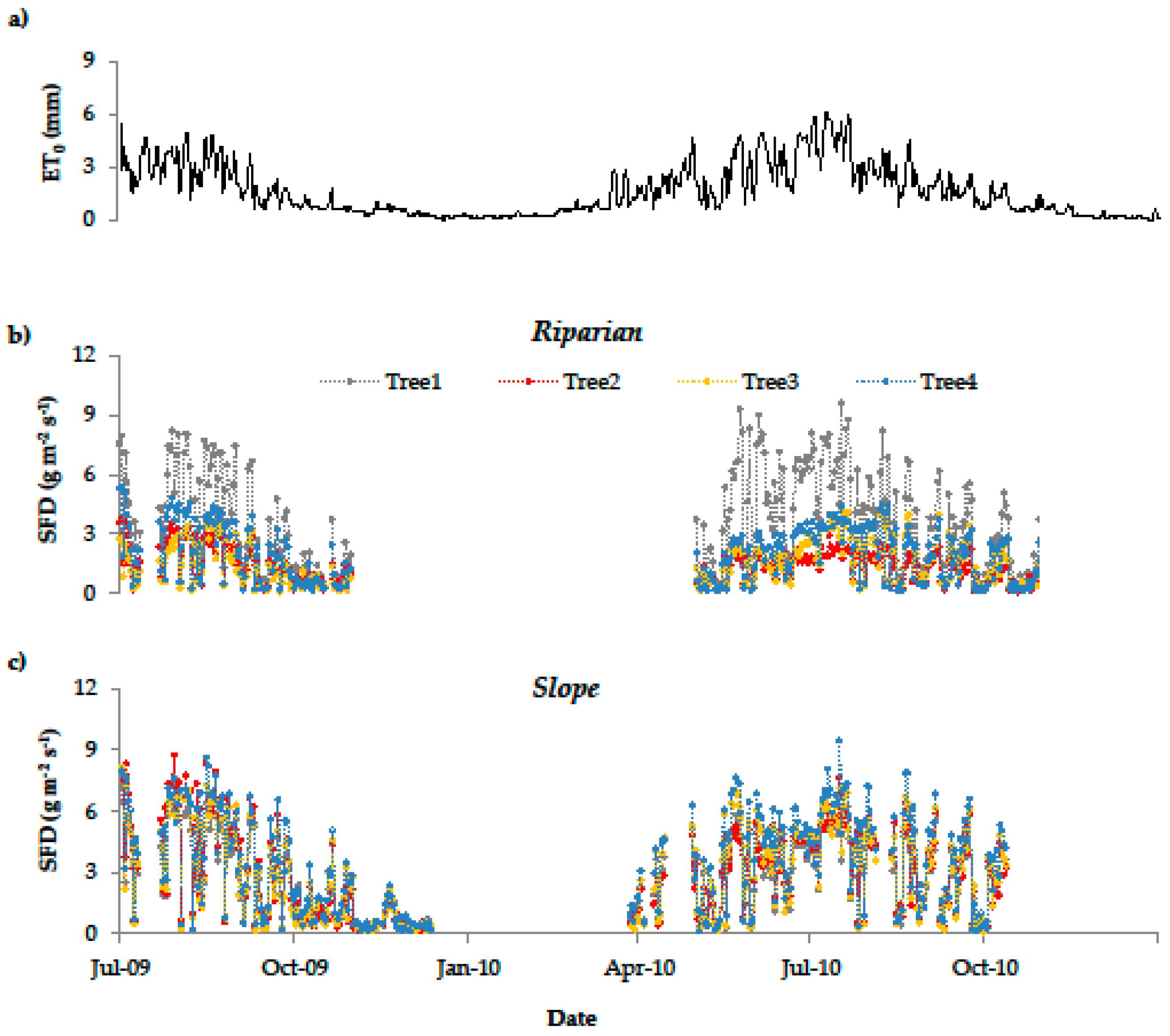
The observed SFD dynamic of both research plots corresponds well to the dynamic of the calculated ET0 (Figure 4). R² between mean daily SFD and ET0 was 0.78 for the Slope plot and 0.84 for Riparian plot. The differing absolute SFD among trees and plots result from variations in tree diameter and crown size (Table 1), which can be explained by small-scale variations in planting density and uneven forest thinning. This becomes particularly apparent for tree 1 of the Riparian plot (Figure 4b).
At the Riparian plot, we observed some data inconsistencies in the winter that were probably caused by frost events and rodent activity. Therefore, the sap flow sensors were checked and readjusted at the beginning of the following vegetation period (May 2010). Since we did not use the noisy data until sensor readjustment, the winter gap at the Riparian plot is slightly longer than at the Slope plot (Figure 4).
3.2. Simulated Soil Water Dynamics
The Mualem-van Genuchten parameters as resulting from the parameter estimation by HYDRUS-1D show lower residual, but higher saturated water contents for the Riparian plot than for the Slope plot. At the Slope plot, α and Ks decrease with depth (Table 2).
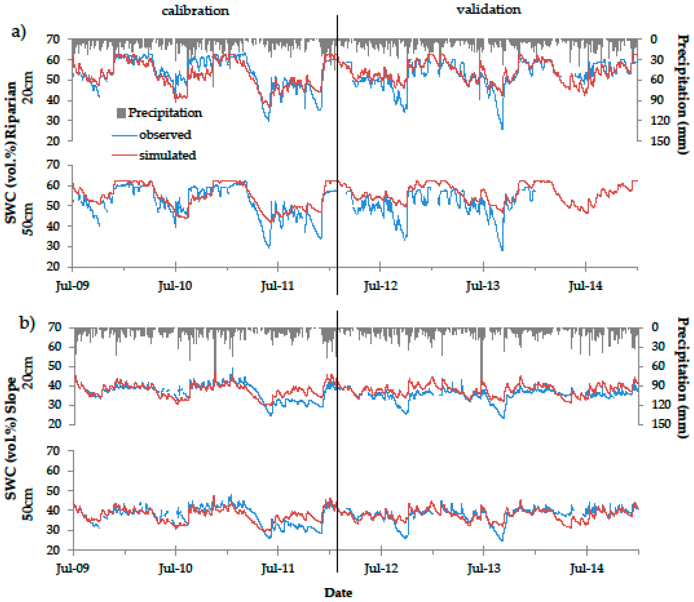
After inverse modelling, and manual calibration of Aqh and Bqh for the deep drainage option (−0.85 and −0.012, respectively), the root mean squared errors (RMSE) between observed and simulated data (Figure 5) were 3.6 vol % (Slope), and 4.6 vol % (Riparian). In the validation period, the RMSE of the Riparian plot slightly increased (5.3 vol %), while that of the Slope remained the same. The manual calibration of the Feddes parameters slightly improved the RMSE at the hillslope plot (3.4 vol % for both calibration and validation period), but had no effect on the RMSE of the Riparian plot simulations.
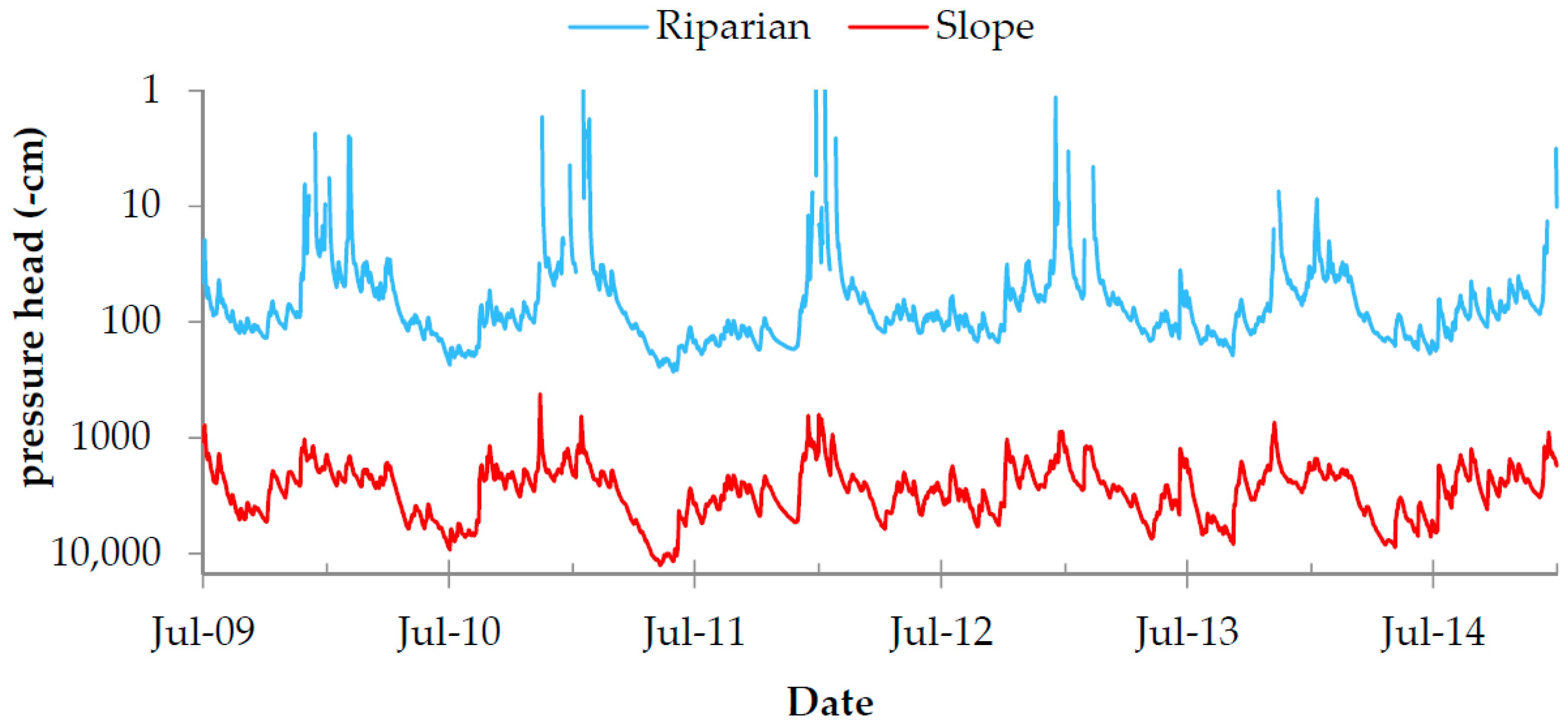
As expected, SWC in the groundwater-influenced plot (Riparian) were generally higher than those on the hillslope. The simulated mean annual SWC was 54% for the Riparian plot and 36% for the Slope). The simulated root zone water potentials (Figure 6) highlight the contrasting soil moisture regimes of the two research plots. The mean simulated annual root zone pressure heads were −88 cm (Riparian) and −3400 cm (Slope). All simulated daily root-zone h values ranged from +27 cm (fully saturated soil column; Riparian) to −12,577 cm (very dry conditions near wilting point; Slope).
3.3. Feddes Parameters for Norway Spruce (h1, h2, h3,low, h4)
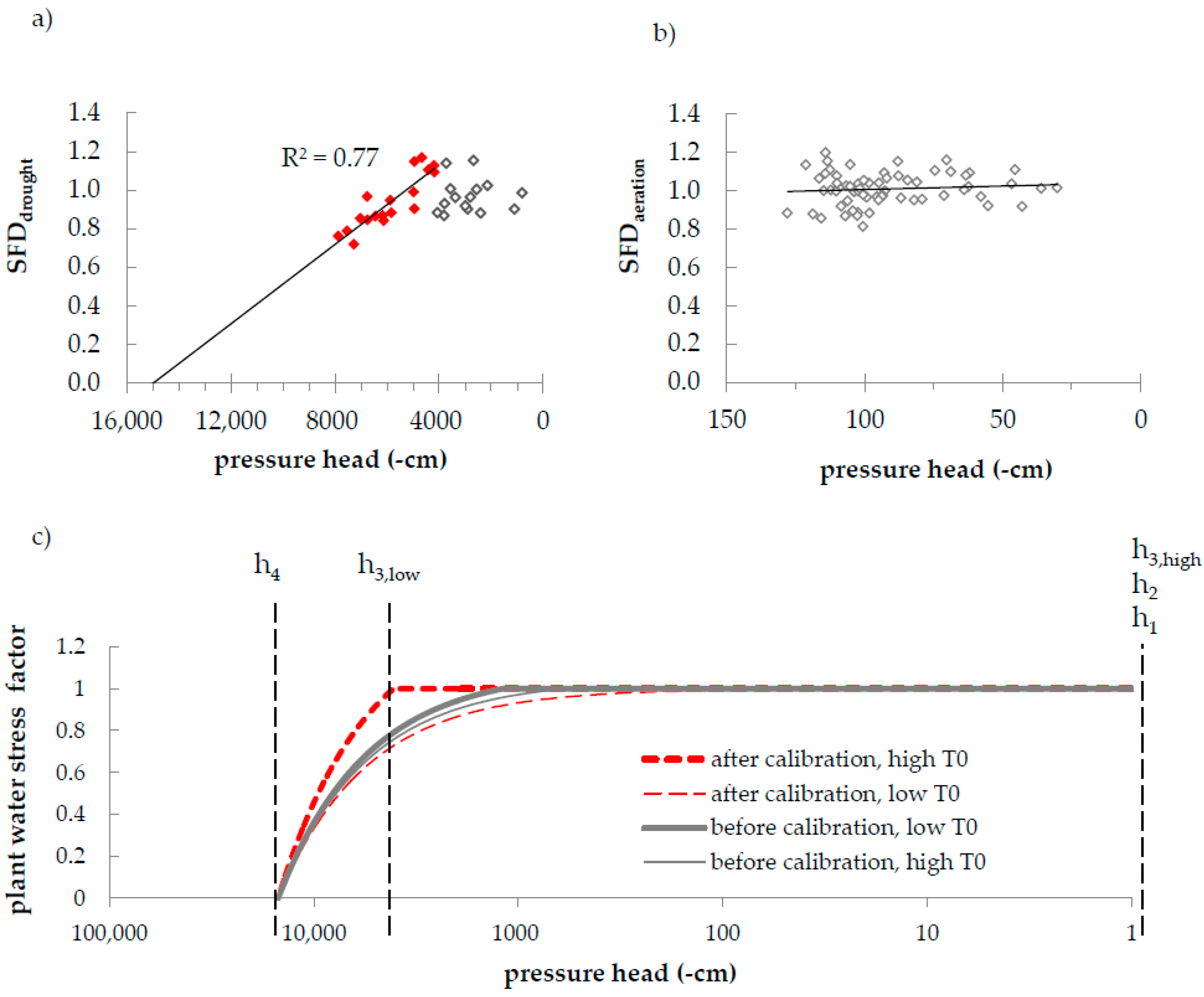
For the Slope plot, we found the measured water stress to be dependent on the simulated root-zone water potential (Figure 7a). The strongest significant correlation between SFDdrought and simulated root-zone h was observed below −4100 cm (R² = 0.77, p < 0.001). Thus, we set h3,low = −4100 cm. Extrapolating the trend-line between SFDdrought and simulated root-zone h towards the x-axis, where SFDdrought = 0 (maximum water stress), resulted in an h4 value of −15,000 cm which is often used as—a very general—permanent wilting point [68]. Our data did not indicate the occurrence of aeration stress at our research site (Figure 7b). Parameters h1 and h2 were therefore set to 0. The Feddes water stress function as resulting from our parameterization shows a higher drought resistance of Norway spruce than previously assumed (Figure 7c).
3.4. Simulated Water Balance before and after Calibration
The mean annual simulated water balance of the two research plots indicates generally higher transpiration at the Riparian plot compared to the Slope plot (Table 3). While the water balance of the Riparian plot was not affected by the calibration of the Feddes parameters, the calibration raised ETact by 10% for the Slope plot. At the same time, drainage decreased by 5%. For all simulation runs, we achieved a very good fit between mean daily sap flow and simulated actual transpiration (R² = 0.82 at Slope and 0.84 at Riparian plot). At the Slope plot, the correlation between sap flow data and simulated actual transpiration was slightly improved by the calibration of the Feddes parameters (R² = 0.83). For the Riparian plot, R² was not affected from the calibration.
3.5. Sensitivity of Feddes Parameters to Root Zone Variation and SoilNet Measuring Location
Variations of the potential root water uptake factor’s depth distribution did not lead to significant variations of the simulated root zone h (Mann-Whitney U-test). The same applies for variation of the rooting depths.
The difference between the mean soil water supply of the surrounding SoilNet measuring locations and that of the stations we selected for our study (SN17 and SN28; cf. Figure 1) was statistically significant (p < 0.001). However, the absolute difference among the simulated SoilNet locations was small and the contrasting soil moisture regimes between the two plots are still clearly visible (Figure 8). Respectively, the resulting Feddes parameters were only slightly affected by the selection of the SoilNet measuring location. Parameter h3,low as determined from the mean root zone water potentials of the surrounding SoilNet locations was −3800 cm, which is 300 cm below the h3,low value we determined from SN28. h4 decreased from −15,000 cm (SN28) to −13,600 cm pressure head (mean of the surrounding SoilNet stations), while h2 was not affected from the choice of the SoilNet measuring location. This indicates that soil type and elevation were reasonable criteria for the choice of our measuring locations.
4. Discussion
4.1. Soil Moisture Simulations
The water balance simulation captured the prevailing soil moisture dynamics reasonably well. Considering the measurement uncertainty of the installed SWC sensors (4–5 vol %; [37]) the RMSE of 3.4 to 5.3 vol % appear very low and are within the range of other HYDRUS-1D studies on the Wüstebach test site [50,53]. The varying soil hydraulic properties among plots and layers (Table 2) fit well to the observations of [36,38]. The low Ks value in the riparian zone is plausible, because the soils in the valley bottom have a higher bulk density and a lower macro-porosity than the soils on the hillslopes [37,38].
The simulated mean annual root-zone water potentials (Figure 6) highlight the contrasting soil moisture regimes of our research plots (wet and dry). These characteristics become even more pronounced when referring only to the vegetation periods (May-September), where mean root-zone pressure heads are −124 (Riparian) and −4308 cm (Slope). Covering particularly the stages of critical soil water supply (undersupply/oversupply) our data seems very suitable for investigating the on-set of drought and aeration stress in plants.
4.2. Water Stress Response of Norway Spruce
There is evidence that the shallow rooting Norway spruce is more vulnerable to drought than other species with a deeper rooting system [4,23,69]. Also, [4,25] found the sap flow activity of Norway spruce to decouple from climate variables with increasing soil water shortage. However, critical levels of soil water supply that induce a decline in sap flow rates and transpiration considerably vary among studies.
While [4] observed gradually decreasing sap flow rates with increasing soil water shortage for REW < 0.4 (which corresponds to a pressure head of −3240 cm at our Slope plot), [23] found Norway spruce to be more drought resistant. Depending on the soil depth considered, they report mean critical REW values of between 0.21 (0–20 cm) and 0.24 (0–50 cm). However, the observed critical REW level strongly varied among trees (REW: 0.18–0.37), which [23] attribute to the heterogeneous soil conditions on site. This is in line with [4], who found the stress response of Norway spruce to become increasingly variable between individuals with continuing drought stress. Comparing the water stress response of Norway spruce among more than 60 pure and mixed stands, [24] report difficulties in determining a consistent critical level of REW. For most of the plots, drought limitation of sap flow began around a REW of 0.3. However, the data scatter around this critical limit was large and a clear decrease in transpiration for all stands except peat stands was only observed for REW below 0.25.
In simulation studies, a REW level of 0.3–0.4 is commonly used to indicate the on-set of drought stress in Norway spruce [31,61,62]. However, this critical REW range is widely accepted for many species (not only for spruce) and our data show that REW does not represent the actual energy state of the soil. For example, at the Slope plot a REW value of 0.3 corresponds to a root-zone pressure head of −4680 cm, which is in the same range (pF 3.7) as the critical h value of −4100 cm (pF 3.6) we observed in our study (Figure 7a). However, a REW threshold of 0.3 at the Riparian corresponds to a root-zone pressure head of −2140 cm suggesting that drought stress would occur much easier at this site (i.e., at lower soil matric potentials). On the other hand, a critical root-zone water potential of −4100 cm pressure head would here correspond to a REW of 0.17.
One could argue that the poor fit between our critical h and the critical reported REW values for the Riparian plot is of minor importance, because critical water contents are never reached [24,70]. Moreover, the concept of REW seems to apply fairly well to the conditions at the Slope plot and to other soils in central European high and low mountain ranges [4,31,61,62]. However, Norway spruce is also widely distributed in boreal forest landscapes, where typical critical REW values seem to be lower than 0.3 [23,24] and soils are often peaty [71], hence showing similar characteristics (low residual water content, high saturated water content; [72,73,74]) as our plot in the riparian zone. Our data indicates that for such soils the concept of REW is likely to fail. This emphasizes the value of soil water potential in comparison to other measures of soil water supply, because, respective water stress thresholds can be applied to any type of soil as long as soil water retention and plant characteristics are known.
However, while critical soil water potentials have been determined for many agricultural crops, little effort has been put into the quantification of Feddes parameters for forest trees. To our knowledge, the concept of transpiration limiting soil water potentials has hardly been applied in spruce site simulation studies. In the few studies we found, the drought stress threshold was generally assumed to be less negative than the value we determined from our sap flow data (h3,low = −4100 cm).
Huang et al. [75] set h3 to the root-zone h at a SWC of 27.5% of the SWC at field capacity. This corresponds to the mean critical SWC they reviewed from different studies on drought-stress in evergreen tree species. Applied to our data and considering field capacity to be represented by SWC at −300 cm pressure head (see above), this threshold corresponds to a pressure head of −3890 cm at the Riparian plot, but to h < −10 million cm at the Slope site, which is far below the common used value for the permanent wilting point. Dependent on the soil type, Rosenqvist et al. [76] assumed the onset of drought stress for Norway spruce at water potentials of −500 (coarse sandy soils) to −1000 cm pressure head (clayey soils). However, these texture dependent water stress thresholds contradict the idea that the soil water potential is already a function of SWC and soil properties. From a plant physiological perspective, species-specific water stress thresholds should be used instead. Vogel et al. [59] set their drought stress thresholds to −1200 (h3,low) and −600 cm pressure head (h3,high). These parameters were derived from other hydrological studies that were conducted on similar soils, but had no plant physiological basis. Nevertheless, applying the parameter set of [59] to our simulations, we achieved a very good fit between measured and simulated SWC (RMSE < 5.3 vol %). Also, mean daily sap flow and simulated actual transpiration showed high correlations (R² > 0.82). However, although the adaptation of the Feddes function had little impact on the general dynamic of the simulated fluxes, the adjustment of h3, low significantly changed transpiration (p < 0.001) and drainage fluxes (p < 0.01) at the Slope plot (two-sided Mann-Whitney U-test; Table 3) and made it more realistic: Based on eddy-covariance measurements, [40] found the annual ETact in the Wüstebach catchment to cover approximately 90% of ET0. In our Slope plot simulations this ratio was 80% for the uncalibrated Feddes model, but 87% for the calibrated simulation run in the samestudy period (2010–2013). The runoff ratio (runoff/precipitation) observed by [40] was 56%, while that in our simulations ranged between 62% (Slope plot after calibration of the Feddes model) and 65% (Slope plot before calibration of the Feddes model). This result confirms: (1) the finding of [77] that a good fit between simulated and measured SWC does not necessarily imply that the simulated water fluxes are correct; and (2) the assumption of [78] that sap flow measurements can help improving root water uptake simulations.
It has to be noted that the impacts of the Feddes model on simulated water fluxes depend on local site conditions. The well-watered Riparian plot was not affected by the calibration, because critical pressure heads were never reached. Drought stress simply did not occur and although there is evidence on the vulnerability of Norway spruce to waterlogging [4,79], our data did not indicate arising aeration stress in the riparian zone (Figure 7b). One reason could be that spruce indeed only suffers from aeration stress at fully saturated soils (h1 = h2 = 0), which does not apply to the vegetation periods in this study (Figure 5). Another possible explanation is that the transpiration limiting effects of aeration stress occur on longer time-scales than the daily scale we were operating at.
Our data show that soil water supply strongly influences the transpiration of Norway spruce. Due to the observed drought stress on the hillslope (Figure 7a), the simulated actual transpiration at the Slope plot was 13% lower than that of the riparian zone (Table 3). This result highlights the importance of considering soil moisture patterns in the modeling of transpiration fluxes from the forest plot to the catchment scale.
5. Conclusions
In this study, we confirm the potential of sap flow measurements for the determination of water stress in forest trees. By combining soil hydrological simulations with a water stress factor derived from sap flow data, we were able to parameterize the Feddes water stress function for Norway spruce and improve our water balance simulations on site. Our results show that small-scale variations in soil water supply significantly influence the water balance of spruce sites. Considering soil moisture patterns in the model setup can thus improve the simulation of transpiration fluxes on the catchment scale.
Although additional sap flow stations and a bigger sample size per plot would have provided a more detailed view on the conditions on site, the sampling concept (wet plot against dry plot) delivered valuable insights into the water stress response of Norway spruce. The advantage of our sampling approach is that an upscaling of sap flow density to the tree and plot scale is unnecessary. Hence, uncertainties related to the upscaling procedure (cf. e.g., [7,66,67,68,69,70]) can be avoided. However, to transfer our finding to other sites and settings, more research on species-specific feedbacks in the soil-vegetation-atmosphere system is needed. There is still a lack of studies determining the critical limits of soil water supply for trees. Since forests play a vital role in regional and trans-regional water cycles and, against the background of climate change, the assessment of respective fluxes becomes increasingly important, future research should focus on: (1) more species-specific investigations on the water stress response of trees; and (2) an improved assessment of small-scale variabilities in soil water supply. With our sampling strategy, we present a simple and cost-efficient approach to achieve these goals, even with a limited number of sample trees.
Acknowledgments
The authors thank the DWD (Deutscher Wetterdienst, German Meteorological Service) and TERENO (Terrestrial Environmental Observatories, funded by the Helmholtz-Gemeinschaft) for providing soil and weather data for this study; we thank DFG (Deutsche Forschungsgemeinschaft) for financial support of sub-project C1 of the Transregional Collaborative Research Center 32 “Patterns in Soil-Vegetation-Atmosphere Systems” and for covering the costs to publish in this journal. Many thanks to Alexander Graf and Inge Wiekenkamp for computing grass reference evapotranspiration and thanks to Michael Röös and Hans-Joachim Spors (Eifel National Park) for their cooperation and the necessary research permits.
Author Contributions
All authors conceived and designed the experiments; Inken Rabbel performed the experiments, analyzed the data and wrote the paper.
Conflicts of Interest
The authors declare no conflict of interest.
References
- Boyer, J.S. Water Transport. Annu. Rev. Plant Physiol. 1985, 36, 473–516. [Google Scholar] [CrossRef]
- Asbjornsen, H.; Goldsmith, G.R.; Alvarado-Barrientos, M.S.; Rebel, K.; Van Osch, F.P.; Rietkerk, M.; Chen, J.; Gotsch, S.; Tobón, C.; Geissert, D.R.; et al. Ecohydrological advances and applications in plant-water relations research: A review. J. Plant Ecol. 2011, 4, 3–22. [Google Scholar] [CrossRef]
- Blum, A. Plant Breeding for Water Limited Environments; Springer: New York, NY, USA, 2011. [Google Scholar]
- Gartner, K.; Nadezhdina, N.; Englisch, M.; Čermak, J.; Leitgeb, E. Sap flow of birch and Norway spruce during the European heat and drought in summer 2003. For. Ecol. Manag. 2009, 258, 590–599. [Google Scholar] [CrossRef]
- Kool, D.; Agam, N.; Lazarovitch, N.; Heitman, J.L.; Sauer, T.J.; Ben-Gal, A. A review of approaches for evapotranspiration partitioning. Agric. For. Meteorol. 2014, 184, 56–70. [Google Scholar] [CrossRef]
- Wullschleger, S.D.; Meinzer, F.C.; Vertessy, R.A. A review of whole-plant water use studies in trees. Tree Physiol. 1998, 18, 499–512. [Google Scholar] [CrossRef] [PubMed]
- Steppe, K.; Vandegehuchte, M.W.; Tognetti, R.; Mencuccini, M. Sap flow as a key trait in the understanding of plant hydraulic functioning. Tree Physiol. 2015, 35, 341–345. [Google Scholar] [CrossRef] [PubMed]
- Köstner, B.; Granier, A.; Cermák, J. Sapflow measurements in forest stands: Methods and uncertainties. Ann. For. Sci. 1998, 55, 13–27. [Google Scholar] [CrossRef]
- Čermák, J.; Kučera, J.; Nadezhdina, N. Sap flow measurements with some thermodynamic methods, flow integration within trees and scaling up from sample trees to entire forest stands. Trees 2004, 18, 529–546. [Google Scholar] [CrossRef]
- Steppe, K.; De Pauw, D.J.W.; Doody, T.M.; Teskey, R.O. A comparison of sap flux density using thermal dissipation, heat pulse velocity and heat field deformation methods. Agric. For. Meteorol. 2010, 150, 1046–1056. [Google Scholar] [CrossRef]
- Renninger, H.J.; Schäfer, K.V.R. Comparison of tissue heat balance- and thermal dissipation-derived sap flow measurements in ring-porous oaks and a pine. Front. Plant Sci. 2012, 3, 103. [Google Scholar] [CrossRef] [PubMed]
- Lundblad, M.; Lagergen, F.; Lindroth, A. Evaluation of heat balance and heat dissipation methods for sapflow measurements in pine and spruce. Ann. For. Sci. 2001, 58, 625–638. [Google Scholar] [CrossRef]
- Bush, S.E.; Hultine, K.R.; Sperry, J.S.; Ehleringer, J.R. Calibration of thermal dissipation sap flow probes for ring- and diffuse-porous trees. Tree Physiol. 2010, 30, 1545–1554. [Google Scholar] [CrossRef] [PubMed]
- Sun, H.; Aubrey, D.P.; Teskey, R.O. A simple calibration improved the accuracy of the thermal dissipation technique for sap flow measurements in juvenile trees of six species. Trees 2012, 26, 631–640. [Google Scholar] [CrossRef]
- Rabbel, I.; Diekkrüger, B.; Voigt, H.; Neuwirth, B. Comparing ∆Tmax determination approaches for Granier-based sapflow estimations. Sensors 2016, 16, 2042. [Google Scholar] [CrossRef] [PubMed]
- Nadezhdina, N.; Cermák, J.; Ceulemans, R. Radial patterns of sap flow in woody stems of dominant and understory species: Scaling errors associated with positioning of sensors. Tree Physiol. 2002, 22, 907–918. [Google Scholar] [CrossRef] [PubMed]
- Ford, C.R.; McGuire, M.A.; Mitchell, R.J.; Teskey, R.O. Assessing variation in the radial profile of sap flux density in Pinus species and its effect on daily water use. Tree Physiol. 2004, 24, 241–249. [Google Scholar] [CrossRef] [PubMed]
- Gebauer, T.; Horna, V.; Leuschner, C. Variability in radial sap flux density patterns and sapwood area among seven co-occurring temperate broad-leaved tree species. Tree Physiol. 2008, 28, 1821–1830. [Google Scholar] [CrossRef] [PubMed]
- Phillips, N.; Oren, R.; Zimmermann, R. Radial patterns of xylem sap flow in non-, diffuse- and ring-porous tree species. Plant Cell Environ. 1996, 19, 983–990. [Google Scholar] [CrossRef]
- Fiora, A.; Cescatti, A. Diurnal and seasonal variability in radial distribution of sap flux density: Implications for estimating stand transpiration. Tree Physiol. 2006, 26, 1217–1225. [Google Scholar] [CrossRef] [PubMed]
- Cermak, J.; Kucera, J.; Bauerle, W.L.; Phillips, N.; Hinckley, T.M. Tree water storage and its diurnal dynamics related to sap flow and changes in stem volume in old-growth Douglas-fir trees. Tree Physiol. 2007, 27, 181–198. [Google Scholar] [CrossRef] [PubMed]
- Köstner, B.; Falge, E.; Tenhunen, J.D. Age-related effects on leaf area/sapwood area relationships, canopy transpiration and carbon gain of Norway spruce stands (Picea abies) in the Fichtelgebirge, Germany. Tree Physiol. 2002, 22, 567–574. [Google Scholar] [CrossRef] [PubMed]
- Lagergren, F.; Lindroth, A. Transpiration response to soil moisture in pine and spruce trees in Sweden. Agric. For. Meteorol. 2002, 112, 67–85. [Google Scholar] [CrossRef]
- Lundblad, M.; Lindroth, A. Stand transpiration and sapflow density in relation to weather, soil moisture and stand characteristics. Basic Appl. Ecol. 2002, 3, 229–243. [Google Scholar] [CrossRef]
- Střelcová, K.; Kurjak, D.; Leštianska, A.; Kovalčíková, D.; Ditmarová, Ľ.; Škvarenina, J.; Ahmed, Y.A.R. Differences in transpiration of Norway spruce drought stressed trees and trees well supplied with water. Biologia 2013, 68, 1118–1122. [Google Scholar] [CrossRef]
- Arora, V. Modeling vegetation as a dynamic component in soil-vegetation-atmosphere transfer schemes and hydrological models. Rev. Geophys. 2002, 40. [Google Scholar] [CrossRef]
- Van Genuchten, M.T. A Numerical Model for Water and Solute Movement in and below the Root Zone; Research Report No 121; U.S. Salinity Laboratory, USDA, ARS: Riverside, CA, USA, 1987.
- Feddes, R.A.; Kowalik, P.J.; Zaradny, H. Simulation of Field Water Use and Crop Yield; Centre for Agricultural Publishing and Documentaion: Wageningen, The Netherlands, 1978. [Google Scholar]
- Jones, H.G. Monitoring plant and soil water status: Established and novel methods revisited and their relevance to studies of drought tolerance. J. Exp. Bot. 2007, 58, 119–130. [Google Scholar] [CrossRef] [PubMed]
- Verstraeten, W.W.; Veroustraete, F.; Feyen, J. Assessment of Evapotranspiration and Soil Moisture Content Across Different Scales of Observation. Sensors 2008, 8, 70–117. [Google Scholar] [CrossRef] [PubMed]
- Schwärzel, K.; Feger, K.-H.; Häntzschel, J.; Menzer, A.; Spank, U.; Clausnitzer, F.; Köstner, B.; Bernhofer, C. A novel approach in model-based mapping of soil water conditions at forest sites. For. Ecol. Manag. 2009, 258, 2163–2174. [Google Scholar] [CrossRef]
- Šimůnek, J.; Šejna, A.M.; Saito, H.; Sakai, M.; Van Genuchten, M.T. The HYDRUS-1D Software Package for Simulating the Movement of Water, Heat, and Multiple Solutes in Variably Saturated Media; Version 4.17; HYDRUS Software Series 3; Department of Environmental Sciences, University of California Riverside: Riverside, CA, USA, 2013; p. 343. [Google Scholar]
- Bogena, H.R.; Bol, R.; Borchard, N.; Brüggemann, N.; Diekkrüger, B.; Drüe, C.; Groh, J.; Gottselig, N.; Huisman, J.A.; Lücke, A.; et al. A terrestrial observatory approach to the integrated investigation of the effects of deforestation on water, energy, and matter fluxes. Sci. China Earth Sci. 2014, 57, 61–75. [Google Scholar] [CrossRef]
- Zacharias, S.; Bogena, H.; Samaniego, L.; Mauder, M.; Fuß, R.; Pütz, T.; Frenzel, M.; Schwank, M.; Baessler, C.; Butterbach-Bahl, K.; et al. A network of terrestrial environmental observatories in Germany. Vadose Zone J. 2011, 10, 955–973. [Google Scholar] [CrossRef]
- Bogena, H.; Borg, E.; Brauer, A.; Dietrich, P.; Hajnsek, I.; Heinrich, I.; Kiese, R.; Kunkel, R.; Kunstmann, H.; Merz, B.; et al. TERENO: German network of terrestrial environmental observatories. J. Large-Scale Res. Facil. 2016, 52, 1–8. [Google Scholar] [CrossRef]
- Gottselig, N.; Wiekenkamp, I.; Weihermüller, L.; Brüggemann, N.; Berns, A.E.; Bogena, H.R.; Borchard, N.; Klumpp, E.; Lücke, A.; Missong, A.; et al. A three-dimensional view on soil biogeochemistry: A dataset for a forested headwater catchment. J. Environ. Qual. 2017, 46, 210–218. [Google Scholar] [CrossRef] [PubMed]
- Rosenbaum, U.; Bogena, H.R.; Herbst, M.; Huisman, J.A.; Peterson, T.J.; Weuthen, A.; Western, A.W.; Vereecken, H. Seasonal and event dynamics of spatial soil moisture patterns at the small catchment scale. Water Resour. Res. 2012, 48. [Google Scholar] [CrossRef]
- Wiekenkamp, I.; Huisman, J.A.; Bogena, H.R.; Lin, H.S.; Vereecken, H. Spatial and temporal occurrence of preferential flow in a forested headwater catchment. J. Hydrol. 2016, 534, 139–149. [Google Scholar] [CrossRef]
- Sciuto, G.; Diekkrüger, B. Influence of soil heterogeneity and spatial discretization on catchment water balance modeling. Vadose Zone J. 2010, 9, 955–969. [Google Scholar] [CrossRef]
- Graf, A.; Bogena, H.R.; Drüe, C.; Hardelauf, H.; Pütz, T.; Heinemann, G.; Vereecken, H. Spatiotemporal relations between water budget components and soil water content in a forested tributary catchment. Water Resour. Res. 2014, 50, 4840–4847. [Google Scholar] [CrossRef]
- Etmann, M. Dendrologische Aufnahmen im Wassereinzugsgebiet Oberer Wüstebach Anhand Verschiedener Mess- und Schätzverfahren. Diploma Thesis, Westfälische Wilhelms-Universität Münster, Münster, Germany, 2009. [Google Scholar]
- Granier, A. Une nouvelle méthode pour la mesure du flux de séve brute dans le tronc des arbres. Ann. Sci. For. 1985, 42, 193–200. [Google Scholar] [CrossRef]
- Granier, A. Evaluation of transpiration in a Douglas-fir stand by means of sap flow measurements. Tree Physiol. 1987, 3, 309–320. [Google Scholar] [CrossRef] [PubMed]
- Bogena, H.R.; Herbst, M.; Huisman, J.A.; Rosenbaum, U.; Weuthen, A.; Vereecken, H. Potential of wireless sensor networks for measuring soil water content variability. Vadose Zone J. 2010, 9, 1002–1013. [Google Scholar] [CrossRef]
- Allen, R.G.; Pereira, L.S.; Raes, D.; Smith, M. Crop Evapotranspiration: Guidelines for Computing Crop Water Requirements; FAO Irrigation and Drainage Paper 56; FAO: Rome, Italy, 1998. [Google Scholar]
- Cornelissen, T.; Diekkrueger, B.; Bogena, H.R. Significance of scale and lower boundary condition in the 3D simulation of hydrological processes and soil moisture variability in a forested headwater catchment. J. Hydrol. 2014, 516, 140–153. [Google Scholar] [CrossRef]
- Richter, D. Ergebnisse Methodischer Untersuchungen zur Korrektur des Systematischen Meßfehlers des Hellmann Niederschlagsmessers; Berichte des Deutschen Wetterdienstes: Offenbach, Germany, 1995. [Google Scholar]
- Jones, H.G. Physiological aspects of the control of water status in horticultural crops. HortScience 1990, 25, 19–26. [Google Scholar]
- Van Genuchten, M.T. A closed-form equation for predicting the hydraulic conductivity of unsaturated soils. Soil Sci. Soc. Am. J. 1980, 44, 892–898. [Google Scholar] [CrossRef]
- Fang, Z.; Bogena, H.; Kollet, S.; Koch, J.; Vereecken, H. Spatio-temporal validation of long-term 3D hydrological simulations of a forested catchment using empirical orthogonal functions and wavelet coherence analysis. J. Hydrol. 2015, 529, 1754–1767. [Google Scholar] [CrossRef]
- Leterme, B.; Mallants, D.; Jacques, D. Sensitivity of groundwater recharge using climatic analogues and HYDRUS-1D. Hydrol. Earth Syst. Sci. 2012, 16, 2485–2497. [Google Scholar] [CrossRef] [Green Version]
- Hopmans, J.W.; Stricker, J.N.M. Stochastic analysis of soil water regime in a watershed. J. Hydrol. 1989, 105, 57–84. [Google Scholar] [CrossRef]
- Bogena, H.R.; Huisman, J.A.; Baatz, R.; Hendricks Franssen, H.J.; Vereecken, H. Accuracy of the cosmic-ray soil water content probe in humid forest ecosystems: The worst case scenario. Water Resour. Res. 2013, 49, 5778–5791. [Google Scholar] [CrossRef]
- Ammer, C.; Wagner, S. An approach for modelling the mean fine-root biomass of Norway spruce stands. Trees 2005, 19, 145–153. [Google Scholar] [CrossRef]
- Clausnitzer, F.; Köstner, B.; Schwärzel, K.; Bernhofer, C. Relationships between canopy transpiration, atmospheric conditions and soil water availability—Analyses of long-term sap-flow measurements in an old Norway spruce forest at the Ore Mountains/Germany. Agric. For. Meteorol. 2011, 151, 1023–1034. [Google Scholar] [CrossRef]
- Helmisaari, H.-S.S.; Derome, J.; Nöjd, P.; Kukkola, M.; Nojd, P.; Kukkola, M. Fine root biomass in relation to site and stand characteristics in Norway spruce and Scots pine stands. Tree Physiol. 2007, 27, 1493–1504. [Google Scholar] [CrossRef] [PubMed]
- Puhe, J. Growth and development of the root system of Norway spruce (Picea abies) in forest stands: A review. For. Ecol. Manag. 2003, 175, 253–273. [Google Scholar] [CrossRef]
- Schmid, I. The influence of soil type and interspecific competition on the fine root system of Norway spruce and European beech. Basic Appl. Ecol. 2002, 3, 339–346. [Google Scholar] [CrossRef]
- Vogel, T.; Dohnal, M.; Dusek, J.; Votrubova, J.; Tesar, M. Macroscopic modeling of plant water uptake in a forest stand involving root-mediated soil water redistribution. Vadose Zone J. 2013, 12. [Google Scholar] [CrossRef]
- Zweifel, R.; Böhm, J.P.; Häsler, R. Midday stomatal closure in Norway spruce—Reactions in the upper and lower crown. Tree Physiol. 2002, 22, 1125–1136. [Google Scholar] [CrossRef] [PubMed]
- Granier, A.; Bréda, N.; Biron, P.; Villette, S. A lumped water balance model to evaluate duration and intesity of drought constraints in forest stands. Ecol. Model. 1999, 116, 269–283. [Google Scholar] [CrossRef]
- Granier, A.; Loustau, D.; Breda, N. A generic model of forest canopy conductance dependent on climate, soil water availability and leaf area index. Ann. For. Sci. 2000, 57, 755–765. [Google Scholar] [CrossRef]
- Sadras, V.O.; Milroy, S.P. Soil-water treshold for the responses of leaf expansion and gas exchange: A review. Field Crop Res. 1996, 47, 253–266. [Google Scholar] [CrossRef]
- Hentschel, R.; Hommel, R.; Poschenrieder, W.; Grote, R.; Holst, J.; Biernath, C.; Gessler, A.; Priesack, E. Stomatal conductance and intrinsic water use efficiency in the drought year 2003—A case study of a well-established forest stand of European beech. Trees 2016, 30, 153–174. [Google Scholar] [CrossRef]
- Gebauer, T.; Horna, V.; Leuschner, C. Canopy transpiration of pure and mixed forest stands with variable abundance of European beech. J. Hydrol. 2012, 442–443, 2–14. [Google Scholar] [CrossRef]
- Granier, A.; Reichstein, M.; Breda, N.; Janssens, I.A.; Falge, E.; Ciais, P.; Grünwald, T.; Aubinet, M.; Berbigier, P.; Bernhofer, C.; et al. Evidence for soil water control on carbon and water dynamics in European forests during the extremely dry year: 2003. Agric. For. Meteorol. 2007, 143, 123–145. [Google Scholar] [CrossRef]
- Widlowski, J.-L.; Verstraete, M.; Pinty, B.; Gobron, N. Allometric Relationships of Selected European Tree Species; European Commission: Ispra, VA, Italy, 2003.
- Kirkham, M.B. Field capacity, wilting point, available water, and the nonlimiting water range. Princ. Soil Plant Water Relat. 2014, 153–170. [Google Scholar] [CrossRef]
- Cienciala, E.; Lindroth, A.; Cermák, J.; Hällgren, J.-E.; Kucera, J. The effects of water availability on transpiration, water potential and growth of Picea abies during a growing season. J. Hydrol. 1994, 155, 57–71. [Google Scholar] [CrossRef]
- Calder, I.R. Water use by forests, limits and controls. Tree Physiol. 1998, 18, 625–631. [Google Scholar] [CrossRef] [PubMed]
- Bonan, G.B.; Shugart, H.H. Environmental factors and ecological processes in boreal forests. Annu. Rev. Ecol. Syst. 1989, 20, 1–28. [Google Scholar] [CrossRef]
- Rezanezhad, F.; Price, J.S.; Quinton, W.L.; Lennartz, B.; Milojevic, T.; Van Cappellen, P. Structure of peat soils and implications for water storage, flow and solute transport: A review update for geochemists. Chem. Geol. 2016, 429, 75–84. [Google Scholar] [CrossRef]
- Weber, T.K.D.; Iden, S.C.; Durner, W. A pore-size classification for peat bogs derived from unsaturated hydraulic properties. Hydrol. Earth Syst. Sci. 2017, 21, 6185–6200. [Google Scholar] [CrossRef]
- Schwärzel, K.; Šimůnek, J.; Van Genuchten, M.T.; Wessolek, G. Measurement and modeling of soil-water dynamics and evapotranspiration of drained peatland soils. J. Plant Nutr. Soil Sci. 2006, 169, 762–774. [Google Scholar] [CrossRef]
- Huang, M.; Lee Barbour, S.; Elshorbagy, A.; Zettl, J.; Cheng Si, B. Water availability and forest growth in coarse-textured soils. Can. J. Soil Sci. 2011, 91, 199–210. [Google Scholar] [CrossRef]
- Rosenqvist, L.; Hansen, K.; Vesterdal, L.; van der Salm, C. Water balance in afforestation chronosequences of common oak and Norway spruce on former arable land in Denmark and southern Sweden. Agric. For. Meteorol. 2010, 150, 196–207. [Google Scholar] [CrossRef]
- Diekkrüger, B.; Söndgerath, D.; Kersebaum, K.C.; McVoy, C.W. Validity of agroecosystem models a comparison of results of different models applied to the same data set. Ecol. Model. 1995, 81, 3–29. [Google Scholar] [CrossRef]
- Vereecken, H.; Huisman, J.A.; Bogena, H.; Vanderborght, J.; Vrugt, J.A.; Hopmans, J.W. On the value of soil moisture measurements in vadose zone hydrology: A review. Water Resour. Res. 2010, 46, 1–21. [Google Scholar] [CrossRef]
- Tjoelker, M.G.; Boratyński, A.; Bugala, W. Biology and Ecology of Norway Spruce; Springer: Dordrecht, The Netherlands, 2007. [Google Scholar]
Figure 1.
Overview of the Wüstebach test site and its location in Germany. The research plots (Riparian, Slope) cover differing soil types and topographic situations, which results in contrasting soil moisture regimes (wet and dry). The grey dots indicate the SoilNet sensor network of which two stations have been selected for this study (yellow dots). Black dots show the SoilNet stations we selected to analyze soil moisture variability around the sap flow stations. The difference between the displayed contour lines is 2.5 m.

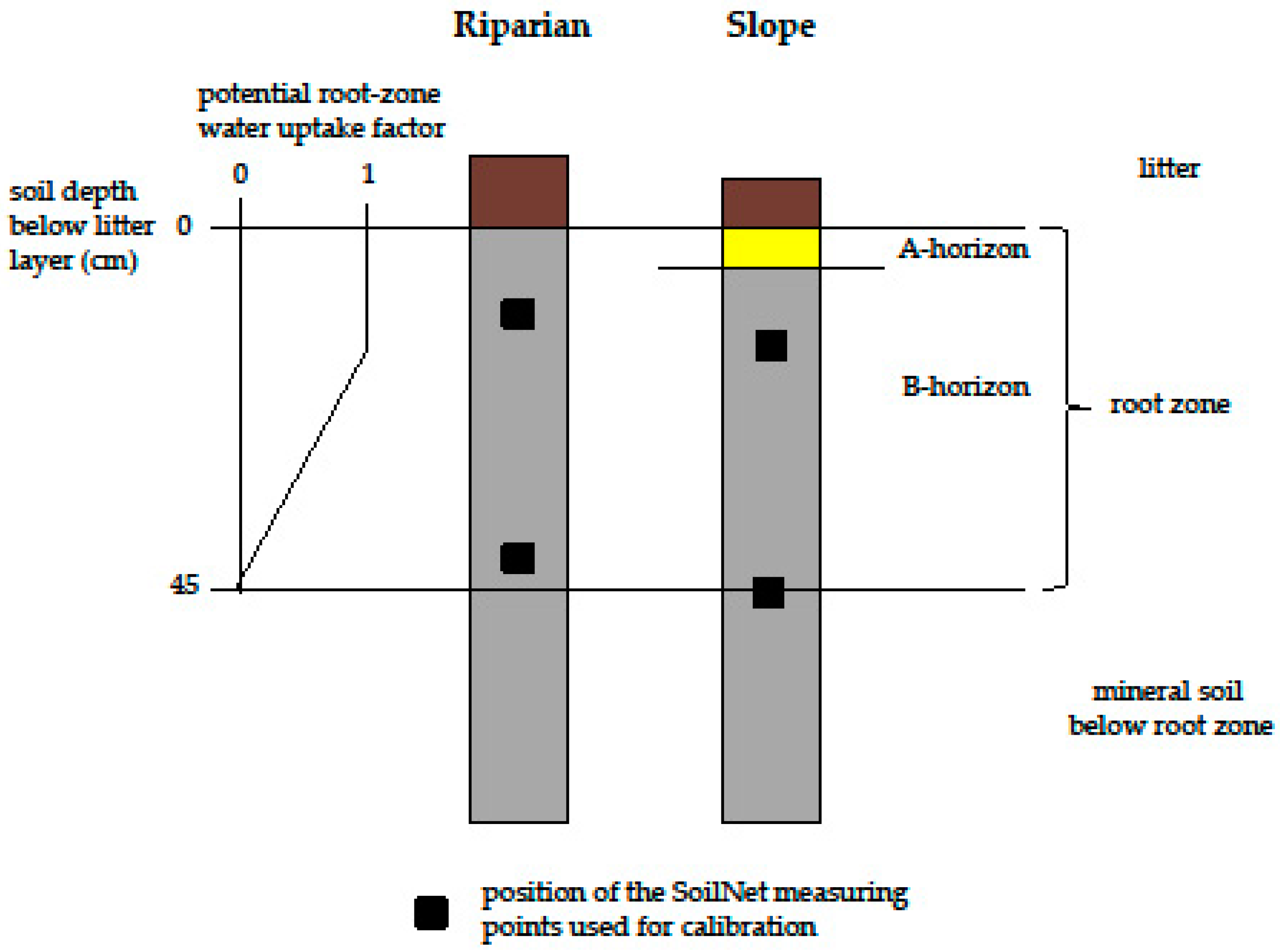
Figure 2.
Upper part of the soil columns of the research plots as discretized in HYDRUS-1D and position of the SoilNet sensors (black dots) in 20 and 50 cm depth below soil surface. The A horizon at the Riparian plot was very thin and therefore neglected in the parameterization.
Figure 2.
Upper part of the soil columns of the research plots as discretized in HYDRUS-1D and position of the SoilNet sensors (black dots) in 20 and 50 cm depth below soil surface. The A horizon at the Riparian plot was very thin and therefore neglected in the parameterization.

Figure 3.
Feddes plant water stress function modified after [28]. Root water uptake commences with the onset of desaturation at h1 (anoxic moisture conditions), optimum root water uptake is given between h2 (field capacity, FC) and h3 (onset of drought-stress), where indiceshigh and low refer to the magnitude of potential transpiration rates. From optimum root water uptake towards h4 (permanent wilting point, WP) the plants experience increasing drought stress.

Figure 4.
Daily potential evapotranspiration (a) and mean daily sap flow density (SFD) by tree and plot ((b) Riparian; (c) Slope).
Figure 4.
Daily potential evapotranspiration (a) and mean daily sap flow density (SFD) by tree and plot ((b) Riparian; (c) Slope).

Figure 5.
Observed (blue) and simulated (red) soil water content (SWC) in 20 and 50 cm depth of the Riparian (a) and Slope (b) plots. Black vertical lines indicate the border between calibration and validation periods.
Figure 5.
Observed (blue) and simulated (red) soil water content (SWC) in 20 and 50 cm depth of the Riparian (a) and Slope (b) plots. Black vertical lines indicate the border between calibration and validation periods.

Figure 6.
Simulated root zone water potential by plot. Note that the pressure head (-cm) is plotted on the log-scale (single positive values cannot be shown).
Figure 6.
Simulated root zone water potential by plot. Note that the pressure head (-cm) is plotted on the log-scale (single positive values cannot be shown).

Figure 7.
(a) Plant water stress as indicated by sap flow data at the Slope plot; red dots were used for the extrapolation of the drought-stress trend-line (black line); (b) Plant water stress as indicated by sap flow data at the Riparian plot (no water stress observed); (c) Calibrated water stress function (red lines) in comparison to the Feddes function used before calibration (grey lines) (cf. [20]). Note that the x-axis in figure (c) is displayed on the log-scale.

Figure 8.
Range (grey) and means (red) of simulated root zone water potentials of the SoilNet stations in the surrounding of our sap flow plots (cf. Figure 1). Simulated root zone water potentials of SN17 (Riparian) and SN28 (Slope) are shown in black. Note that the pressure head (-cm) is plotted on the log-scale (single positive values cannot be shown).


Table 1.
Variation of diameter at breast height (DBH), sap wood depth (SWD), projected crown area (CA) and mean daily sap flow density between May and September (SFD) by plot and sample tree.
Table 1.
Variation of diameter at breast height (DBH), sap wood depth (SWD), projected crown area (CA) and mean daily sap flow density between May and September (SFD) by plot and sample tree.
| Sample Tree | Riparian | Slope | ||||||
|---|---|---|---|---|---|---|---|---|
| DBH | SWD | CA | SFD | DBH | SWD | CA | SFD | |
| cm | cm | m² | g m−2 s−1 | cm | cm | m² | g m−2 s−1 | |
| tree 1 | 57 | 6 | 49.2 | 4.48 | 44.7 | 4.7 | 56.3 | 4.52 |
| tree 2 | 40.3 | 4.2 | 23.3 | 2.25 | 40.9 | 4.3 | 60.4 | 5.09 |
| tree 3 | 46.3 | 4.9 | 22.2 | 1.56 | 44.1 | 4.6 | 33.8 | 4.69 |
| tree 4 | 40.4 | 4.2 | - * | 3.13 | 48.2 | 5.1 | - * | 5.24 |
| mean | 46 | 4.8 | 31.6 | 2.9 | 44.5 | 4.7 | 50.2 | 4.89 |
* These trees were cut before our survey on CA determination; therefore we estimated CA from the allometric relationships of [67], where CA = π × (0.6122 + 0.0536 × DBH)².
Table 2.
Mualem-van Genuchten parameters as obtained from the HYDRUS-1D inverse modeling procedure by plot and soil layer. θr: residual water content, θs: saturated water content, α: empirical parameter related to the air-entry pressure value, n: empirical parameter related to the pore size distribution width, Ks saturated hydraulic conductivity (cm day−1).
| Soil Layer | θr | θs | α | n | Ks |
|---|---|---|---|---|---|
| Riparian | |||||
| B * | 0 | 0.63 | 0.008 | 1.58 | 4 |
| Slope | |||||
| A | 0.1 | 0.52 | 0.008 | 1.22 | 165 |
| B | 0.12 | 0.5 | 0.001 | 1.29 | 78 |
* The A horizon was very thin and could therefore not be parameterized for this plot.
Table 3.
Mean annual simulated water balance (October 2009–September 2014) before and after calibration of the Feddes parameters in HYDRUS-1D. Percentage change of calibrated water balance component in comparison to un-calibrated value is given in brackets. ET0: potential evapotranspiration, ETact: actual evapotranspiration; all details in mm year−1.
| Water Balance Component | Riparian | Slope | ||
|---|---|---|---|---|
| Precipitation | 1321 | |||
| ET0 | 597 | |||
| un-calibrated | calibrated | un-calibrated | calibrated | |
| ETact | 597 | 597 | 403 | 445 (+10%) |
| Surface runoff | 54 | 54 | 0 | 0 |
| Drainage | 634 | 634 | 841 | 797 (−5%) |
© 2018 by the authors. Licensee MDPI, Basel, Switzerland. This article is an open access article distributed under the terms and conditions of the Creative Commons Attribution (CC BY) license (http://creativecommons.org/licenses/by/4.0/).
Share and Cite
MDPI and ACS Style
Rabbel, I.; Bogena, H.; Neuwirth, B.; Diekkrüger, B. Using Sap Flow Data to Parameterize the Feddes Water Stress Model for Norway Spruce. Water 2018, 10, 279. https://doi.org/10.3390/w10030279
AMA Style
Rabbel I, Bogena H, Neuwirth B, Diekkrüger B. Using Sap Flow Data to Parameterize the Feddes Water Stress Model for Norway Spruce. Water. 2018; 10(3):279. https://doi.org/10.3390/w10030279
Chicago/Turabian StyleRabbel, Inken, Heye Bogena, Burkhard Neuwirth, and Bernd Diekkrüger. 2018. "Using Sap Flow Data to Parameterize the Feddes Water Stress Model for Norway Spruce" Water 10, no. 3: 279. https://doi.org/10.3390/w10030279
Note that from the first issue of 2016, this journal uses article numbers instead of page numbers. See further details here.