Separating Wet and Dry Years to Improve Calibration of SWAT in Barrett Watershed, Southern California


1
College of Geographical Sciences, Fujian Normal University, Fuzhou 350007, China
2
Fujian Provincial Engineering Research Center for Monitoring and Assessing Terrestrial Disasters, Fujian Normal University, Fuzhou 350007, China
3
State Key Laboratory of Subtropical Mountain Ecology (Funded by Ministry of Science and Technology and Fujian Province), Fujian Normal University, Fuzhou 350007, China
4
Department of Geography, San Diego State University, San Diego, CA 92182-4493, USA
5
Dorset Environmental Science Center, Ontario Ministry of Environment and Climate Change, 1026 Bellwood Acres Road, Dorset, ON P0A 1E0, Canada
*
Author to whom correspondence should be addressed.
Water 2018, 10(3), 274; https://doi.org/10.3390/w10030274
Submission received: 20 January 2018
/
Revised: 16 February 2018
/
Accepted: 26 February 2018
/
Published: 5 March 2018
Abstract
:Hydrological models often perform poorly in simulating dry years in regions with large inter-annual variability in rainfall. We calibrated the Soil and Water Assessment Tool (SWAT) model to dry and wet years separately, using the semi-arid Barrett watershed on the west coast of USA as an example. We used hydrological and meteorological data from 1980–2010 to calibrate the SWAT model parameters, compared the monthly runoff results simulated by SWAT using a traditional calibration for the entire runoff series with results using a calibration with the wet and dry year series, and analyzed differences in the most sensitive parameters between the wet and dry year series. The results showed that (1) the SWAT model calibrated to the entire runoff series produced significant differences in simulation efficiency between the wet years and dry years, with lower efficiency during the dry years; (2) the calibration with separate wet and dry years greatly enhanced the SWAT model’s simulation efficiency for both wet and dry years; (3) differences in hydrological conditions between wet and dry years were represented by changes in the values of the six most sensitive parameters, including baseflow recession rates, channel infiltration rates, Soil Conservation Service (SCS) curve number, soil evaporation, shallow aquifer flow, and soil water holding capacity. Future work can attempt to determine the physical processes that underlie these parameter changes and their impact on the hydrological response of the semi-arid watersheds.
1. Introduction
Distributed hydrologic models are effective tools for studying complex hydrological phenomena in watersheds under the influence of climate change and anthropogenic activities [1]. One of the most important features of a distributed hydrologic model is the spatial heterogeneity of the processes, which can reflect the effects of the spatial heterogeneity of meteorological factors such as precipitation and evaporation, and underlying surface factors, such as topography, soil, and land use, on the hydrological cycle in the watershed [2].
Temporal changes or variability in the watershed condition also affect model performance. Several studies [3,4] have shown differences in the simulation efficiency between the wet and dry seasons using the Soil Water Assessment Tool (SWAT) model, which is a typical and widely-used semi-distributed hydrologic model [5,6,7,8]. Other hydrologic models also show significant differences in simulation efficiency between wet and dry seasons [9,10]. One of the reasons for this is that some model assessment indices, such as the correlation coefficient (R2) and the Nash-Sutcliffe efficiency (NSE), better reflect the hydrological characteristics of wet periods, and the researcher cannot ensure that the simulations are acceptable in both wet and dry periods when the simulation of entire runoff series performs well [11]. Therefore, several studies [12,13,14,15] have proposed dividing the observed runoff data into wet and dry seasons for separate calibration. Overall simulation efficiencies were improved by differing amounts. Zhang et al. [15] also suggested that the improvements are more significant for the dry periods. Calibration with separate wet and dry seasons results in different values of the SWAT model parameters between the wet and dry seasons. White et al. altered the code of the SWAT model and allowed the curve number (CN) to be changed with the growing season and the dormant season of plants, which improved the model performance by Nash-Sutcliffe coefficient [12]. At the Little River Experimental Watershed in Georgia, USA, the months were divided into a wet period (runoff coefficient > 0.1) and a dry period (runoff coefficient < 0.1); several parameters had different values during the wet and dry periods, including ALPHA_BF for baseflow, CH_K2 for channel routing, CN2 for curve number, ESCO for soil evaporation, and GWQMN for shallow aquifer flow [13].
Although several studies have suggested that the SWAT model is applicable to semi-arid regions [16], the simulation results are worse than those in wet regions [17,18,19,20]. One of the reasons for this difference is that the inter-annual variabilities of the runoff in arid and semi-arid regions are so large that it is difficult to ensure the simulations are acceptable in both wet and dry years. For example, the simulated monthly runoff of the Sarrath River watershed in Tunisia, Africa [21] used the SWAT model and showed that the simulated runoff was generally higher than the measurements when the runoff was less than 4 m3/s. A simulation of the Colorado River in Mexico with SWAT also overestimated runoff during dry periods [22]. Therefore, for regions with large inter-annual runoff variability, the questions examined in this study are: Do the values of the SWAT model parameters differ between the dry and wet years in a semi-arid watershed? Will calibrating the model for wet and dry years separately significantly improve SWAT’s performance?
This study focused on the Barrett watershed, located in southwestern San Diego, California, on the west coast of the USA, simulated the monthly runoff based on a sensitivity analysis of the SWAT model parameters, analyzed the feasibility of dividing the data into wet and dry years for model calibration, and showed differences in the values of model parameters during wet and dry years, in order to improve the applicability of SWAT model to watersheds with different climates and watershed conditions. Although the separation of wet and dry seasons in a year was researched for SWAT modelling, the separation of wet and dry years for SWAT calibration was rarely reported in the literature.
2. Materials and Methods
2.1. Background on the Barrett Watershed
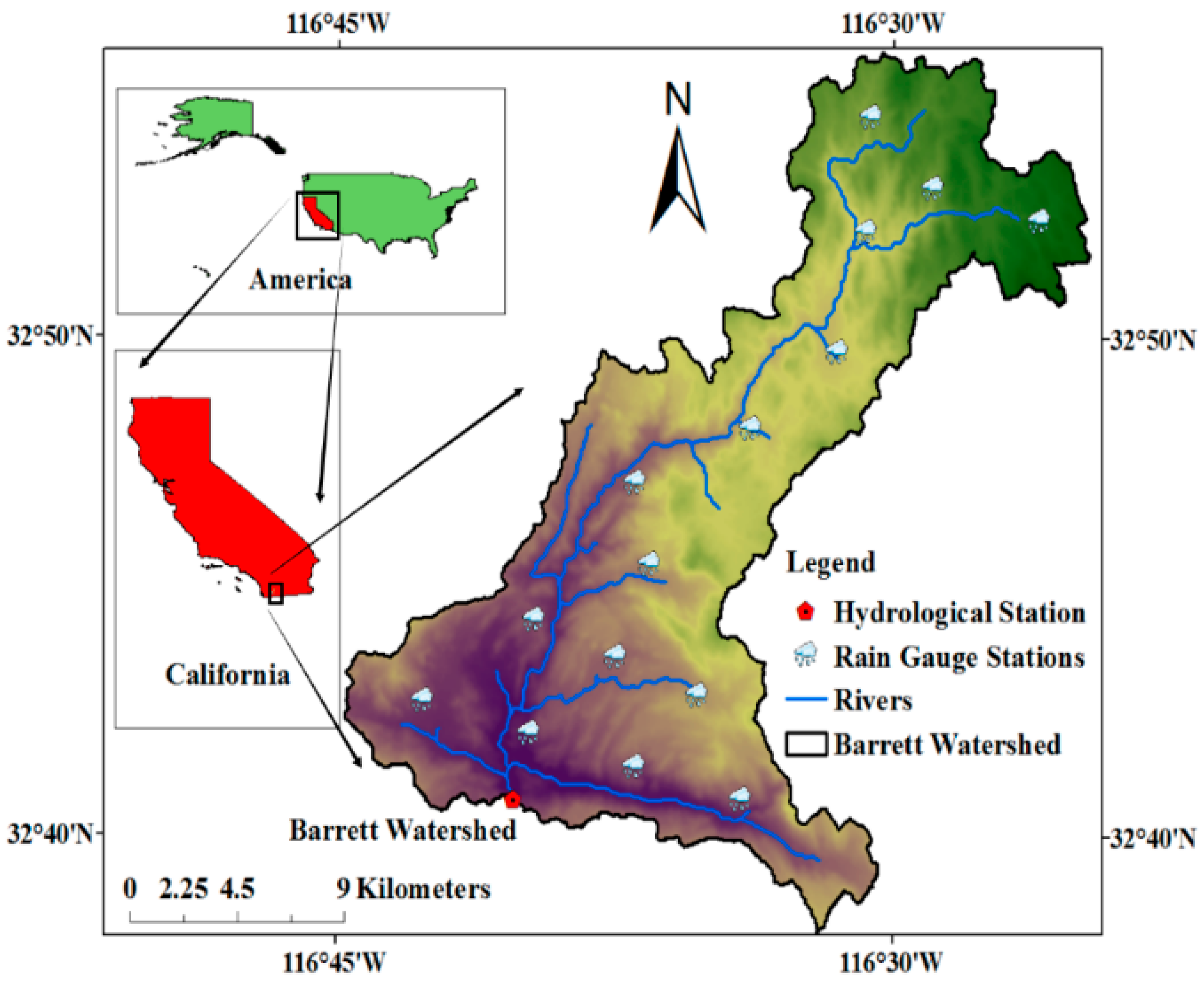
Barrett watershed is part of the Tijuana River watershed along the tributary of the Cottonwood River in USA (Figure 1). The watershed covers an area of 337 km2 and is located between 116°25′–116°48′ W and 32°38′–32°56′ N. Reservoirs in the downstream part of the watershed provide flood control and help meet the industrial and domestic water needs of San Diego [23,24]. The regional land use types are mainly unused land with chaparral vegetation cover and exposed rock followed by forest. Grassland and arable land account for only 3.9% of the total watershed area. Barrett watershed is in a semi-arid climate zone [25], which is hot and dry during the summer and mild and rainy during the winter, and more precipitation occurs at higher elevations. The annual runoff in the Barrett watershed varies significantly, with the coefficient of variation as high as 1.65 during 1901–2010.
2.2. Establishment of the SWAT Model for the Barrett Watershed
2.2.1. SWAT Model Description
The SWAT model [26] is a free, open source, geographic information system-based distributed watershed hydrology model that was developed by the Agricultural Research Service, United States Department of Agriculture (USDA). The water balance in SWAT model is based on following equation:
in which is the final soil water content (mm), is the initial soil water content (mm), t is the time (days), is the amount of precipitation on day i (mm), is the surface runoff on day i (mm), is the amount of evapotranspiration on day i (mm), is the amount of percolation and bypass flow exiting the soil profile bottom on day i (mm), and is the amount of return flow on day i (mm).
The runoff simulation of SWAT model is divided into two main stages: land stage of hydrological cycle and routing stage. The main hydrological processes include surface runoff, interflow (lateral flow), subsurface runoff (groundwater discharge), and river channel routing and infiltration. The surface runoff is calculated with the Soil Conservation Service Curve Number (SCS-CN) method [27] or the Green-Ampt infiltration method [28]; the calculation and re-distribution of the interflow are performed simultaneously considering the spatial-temporal changes of hydraulic conductivity, slope, and soil water content. SWAT divides the groundwater into shallow groundwater and deep groundwater. The shallow groundwater discharges into streams, and the deep groundwater flows outside the watershed. Channel routing is based on the variable storage coefficient model [29] or the Muskingum method [30], and includes channel infiltration.
2.2.2. SWAT Data Sources and General Setting
The input data of SWAT model in Barrett watershed and their sources are as follows:
The topographic 30 m × 30 m DEM data of Barrett watershed were extracted from the Global Digital Elevation Model (GDEM, 30 m resolution) of NASA, which is based on the Advanced Space borne Thermal Emission and Reflection Radiometer (ASTER) and downloaded from the International Scientific Data Service Platform of Chinese Academy of Sciences (Geospatial Data Cloud site, Computer Network Information Center, Chinese Academy of Sciences, http://www.gscloud.cn). The soil data were from the State Soil Geographic (STATSGO) Database of the Natural Resources Conservation Service (NRCS) of USDA. The land use in 2000 was downloaded from the San Diego Geographic Information Source (SanGIS). Based on the actual land use characteristics of Barrett watershed, the authors divided the land use into six types (forest, grassland, arable land, orchard land, construction land, and unused land) and recoded the land use data based on the codes of urban land use and crop growth database of SWAT model.
The meteorological data included daily maximum temperature, minimum temperature, precipitation, solar radiation, wind speed, and relative humidity. Most meteorological data of Barrett watershed were from the 1980–2012 Daymet dataset of the Earth Science Data website of National Aeronautics and Space Administration (NASA) [31]. This dataset was composed of daily 1 × 1 km gridded data with coverage of all North America and included the daily maximum temperature, minimum temperature, precipitation, relative humidity, and solar radiation. Although there are more than 200 grids falling in Barrett watershed, it is not easy to set up the weather database by using all grids. Thus, 15 grids of Daymet dataset distributed uniformly in the watershed were selected as the meteorological input, because these 15 grids cover the watershed (Figure 1) and reflect the spatial distribution of meteorological variables (such as precipitation, temperature, and relative humid) in the watershed. The wind speed data was generated by the weather generator of SWAT, and the monthly inflow of the Barrett Reservoir during 1980–2010 was calculated from the reservoir water balance, which included change in storage, precipitation, evaporation, and seepage losses (unpublished data, City of San Diego).
The watershed was divided into 31 sub-watersheds based on the DEM data and a threshold area of 6 km2. Areas with the same land use, soil type, and slope within a sub-watershed formed a Hydrologic Response Unit (HRU). Minimum thresholds of 5%, 15%, and 15% for land use, soil type, and slope coverage, respectively, were used to define the number of HRUs within any given sub-watershed. As a result, a total of 141 HRUs have been identified for the watershed. The SCS curve number method was selected to calculate surface runoff, and the variable storage coefficient method was used to calculate river routing.
2.2.3. Parameter Sensitivity Analysis
The SWAT model includes numerous parameters. During the model calibration, it is difficult to adjust each parameter to achieve optimal combination of parameters. A sensitivity analysis can be used to select the parameters that are important to the simulation results.
We used the sensitivity analysis module in SWAT2009, which used the Latin Hypercube-One factor At a Time (LH-OAT) sensitivity analysis method [32]. LH-OAT sensitivity analysis, a global sensitivity analysis method, was proposed by Grienseven with a combination of LH sampling method [33] and OAT sensitivity analysis method [34]. It had the advantages of both the LH sampling method and OAT sensitivity analysis, which ensured that all parameters were sampled within the specified ranges; it could clearly identify parameters that led to changes in the model results. The method operates by loops, and each loop starts with a Latin Hypercube point. Around each Latin Hypercube point j, the average of sensitivity index for each parameter is calculated as (in percentage):
in which M( ) refers to the model objective functions, is the fraction by which the parameter is changed (a predefined constant), and refers to a LH point (j ∈ [1, N]).
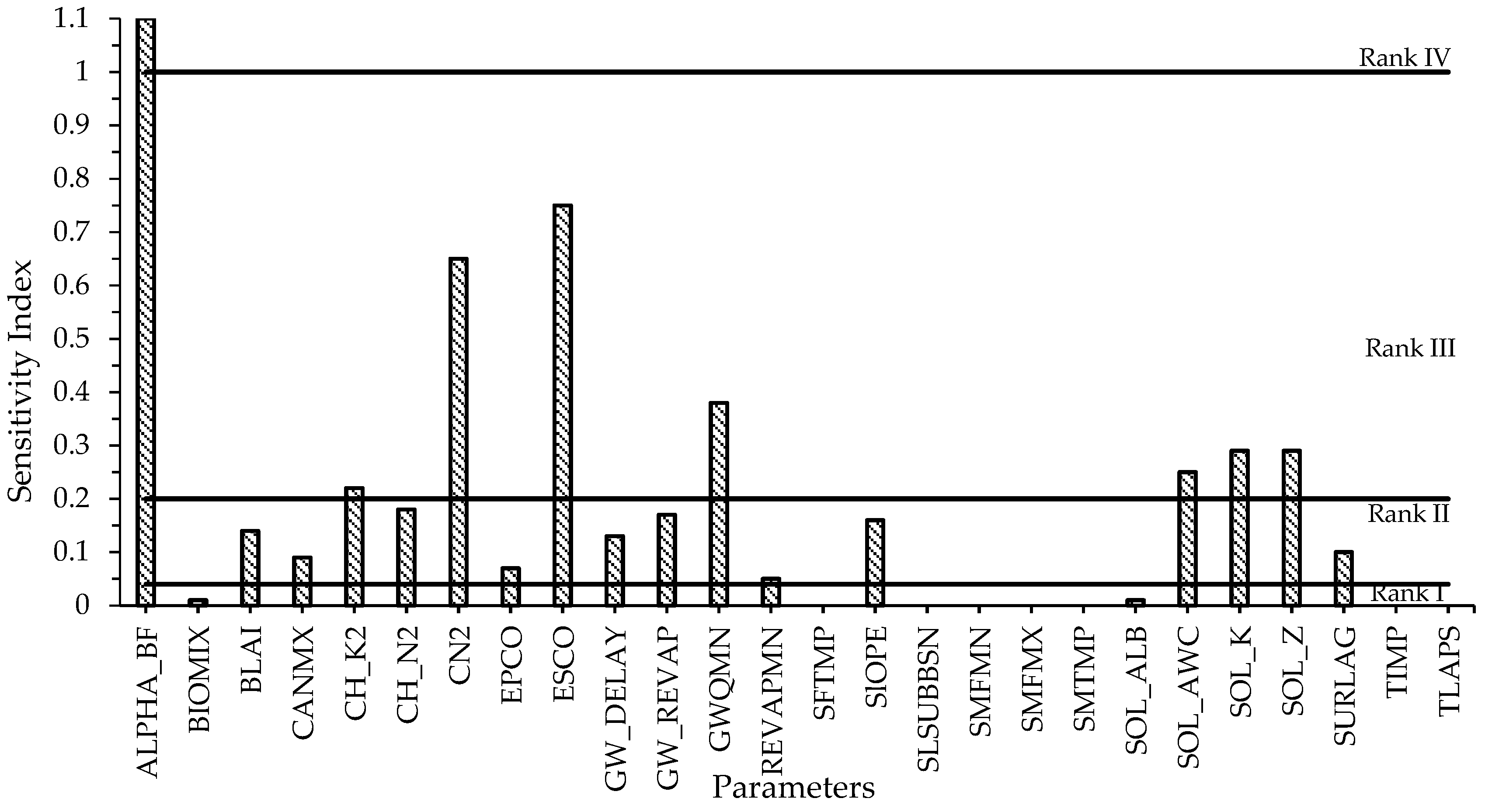
SWAT’s 26 parameters related to the hydrological processes were selected to do a sensitivity analysis. To make the sensitivities of model parameters comparable, the sensitivity index was divided into four ranks: very high, high, medium, and small to negligible (Table 1), with higher sensitivity values indicating higher sensitivity of the parameter [35].
2.2.4. Model Calibration and Validation
SWAT model (SWAT 2009 version) was run on monthly time steps for the period of January 1980 to December 2010 for calibration and validation. After the warm-up year (1980), streamflow records from 1981 to 1995 were used for the calibration period, while the records from 1996 to 2010 were used for the validation period.
Based on the sensitivity analysis, the parameters that had a significant impact on the stream flow were selected to calibrate the model by adjusting the parameters manually and automatically. Sequential Uncertainty Fitting (SUFI-2) [36] was selected as the automatic calibration method, which was used by SWAT-CUP software provided by the official SWAT website.
Nash-Sutcliffe coefficient (NSE), coefficient of determination (R2), and relative error (RE) were used to evaluate the performance of the model. The NSE quantifies the goodness-of-fit of the simulated values relative to the observed values and usually falls in the range of 0–1. The closer the NSE is to 1, the better the goodness-of-fit. NSE < 0 indicates low simulation reliability. R2 reflects the correlation between observed and simulated values and has a range of 0–1. RE is used to measure the average tendency of the simulated values to be larger or smaller than the observed counterparts. The closer RE is to 0, the more accurate the simulated result. RE > 0 means that the simulated value is larger than the observed value, whereas RE < 0 means that the observed value is greater than the simulated value. It has been suggested that simulation results are acceptable when NSE > 0.5, R2 > 0.6, and RE is between ±25% [37].
2.3. Calibration and Validation for Wet and Dry Years
Annual runoff data of Barrett watershed were divided into wet and dry years, and then SWAT was calibrated and validated with the wet-year series and the dry-year series separately.
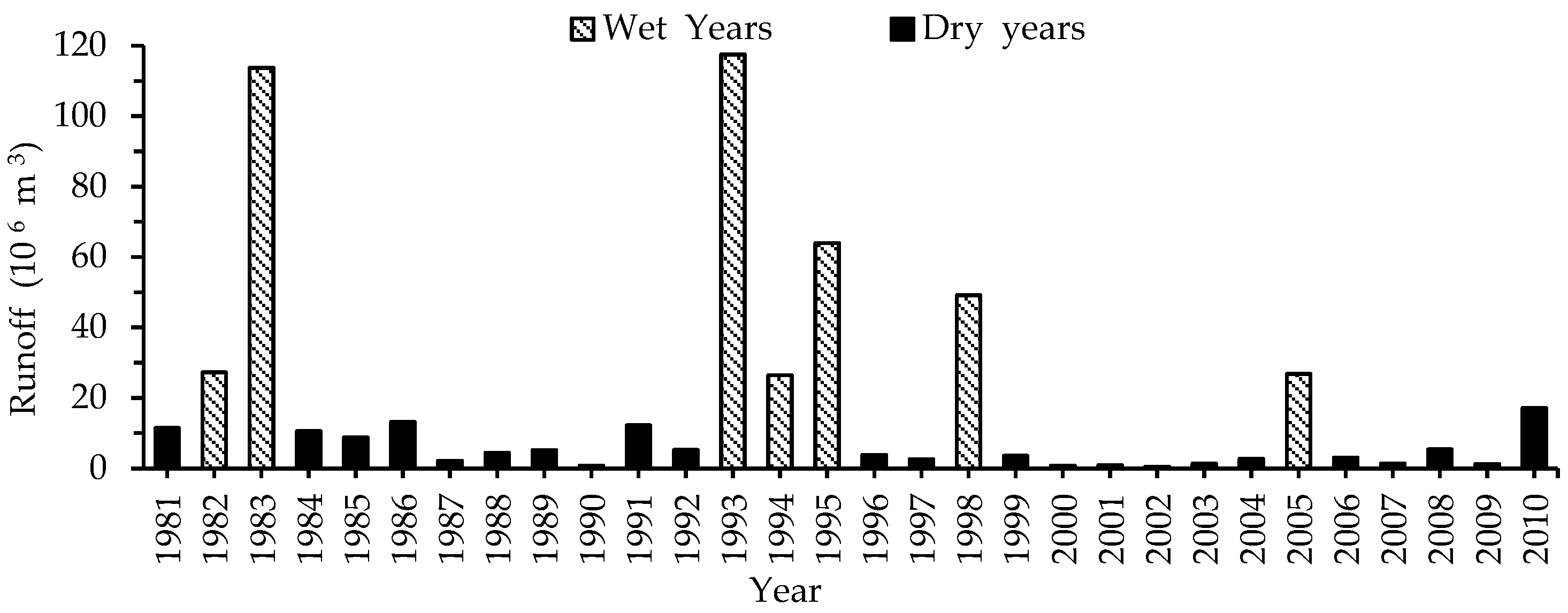
In the Standard for Hydrological Information and Hydrological Forecasting of China (GB/T 22482-2008), a method of “relative deviation percentage” ((annual runoff − mean runoff)/(mean runoff) × 100%) was used to divide wet and dry years with which annual runoff was categorized into five grades (very high flow year, high flow year, normal flow year, low flow year, and very low flow year). Because of large variability of runoff between wet and dry years in Barrett watershed, the five grades were simplified to only two grades of wet yeas and dry years. There is no broadly accepted criterion to judge a wet or dry year, and the separation is relative. For purposes of simplicity and easy application, the long-term mean annual runoff was used as a threshold for this study. Years whose annual runoff was greater than the mean annual runoff over 1981–2010 were identified as wet years, while those that were less than the mean annual runoff were identified as dry years. The whole period included 7 wet years and 23 dry years (Figure 2). Dry years accounted for about two thirds of all years.
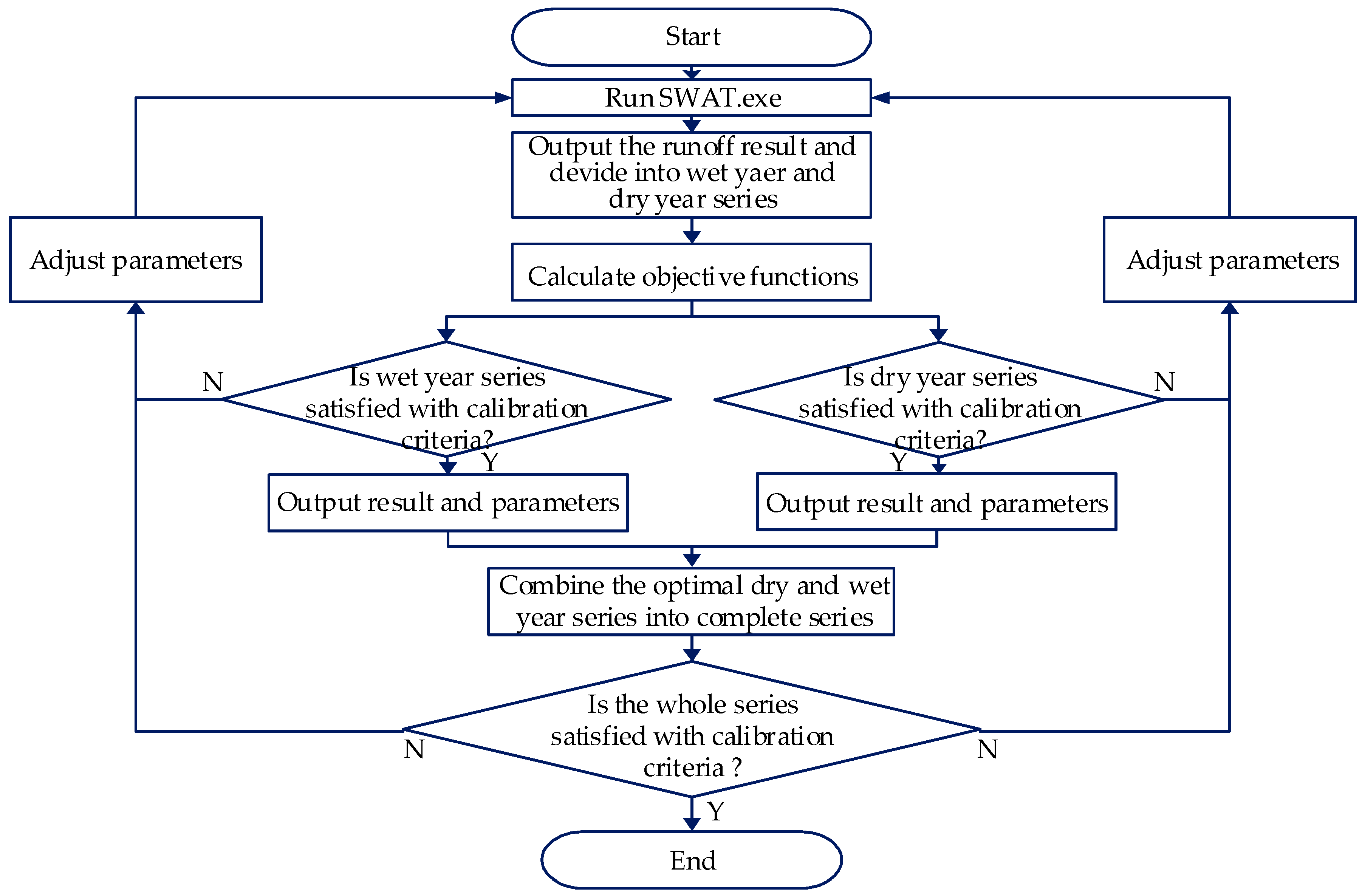
In the model calibration process (1981–1995) with separated wet and dry years (Figure 3), the SWAT- simulated streamflow time series was first divided into wet year series and dry year series after running SWAT.exe. All the objective functions, including R2, RE, and NSE, were calculated for the wet and dry year series separately. Then, the sensitive parameters of wet and dry year series were adjusted separately according to the calculated results of the objective functions, and SWAT model was re-run. These procedures were repeated until both the wet year series and dry year series satisfied the predetermined acceptable conditions of the objective function. The simulated results of wet and dry year series were outputted and combined into a complete series in chronological order. Finally, this process ended when the whole series was checked and seen to conform to the calibration criteria.
At the validation process, for wet years, adjusted parameters of wet year series were inputted into SWAT for simulating runoff in validation period (1996–2010). The simulated runoff in wet years was extracted and used to calculate objective function. If the results were accepted, it showed that the adjusted parameters of wet years were correct. If not, the calibration process was carried out again. The validation process in dry years was the same as that in wet years.
3. Results
3.1. Sensitive Parameters
The results of parameter sensitivity analysis are shown in Figure 4. The LH-OAT sensitivities of most of the 26 hydrological parameters were less than 0.2, corresponding to rank II (medium) or rank I (small to negligible). Eight parameters had sensitivities greater than 0.2, including the baseflow alpha factor (ALPHA_BF), the effective hydraulic conductivity in the channel alluvium (CH_K2), the initial SCS runoff curve number for moisture condition II (CN2), the soil evaporation compensation factor (ESCO), the threshold depth of water in the shallow aquifer required for return flow to occur (GWQMN), the available water capacity of the soil layer (SOL_AWC), the soil saturated hydrologic conductivity (SOL_K), and the depth of soil layer (SOL_Z). The sensitivity of ALPHA_BF, which was greater than 1, is the most sensitive as rank IV (very high). The sensitivities of CH_K2, CN2, ESCO, GWQMN, SOL_AWC, SOL_K, and SOL_Z were between 0.2 and 1, corresponding to rank III (high). These eight parameters played an important role in SWAT simulation for Barrett watershed, including processes of surface water, groundwater, soil evaporation, lateral flow, and channel routing.
3.2. Calibration and Validation of SWAT without Separating the Data
The monthly runoff simulated by SWAT performed well during both the calibration and validation periods, giving NSE, R2, and RE values of 0.86, 0.90, and −7.48% respectively for the calibration, and 0.71, 0.78, and 32.44%, respectively, for the validation (Table 2). They met the goodness criteria (NSE > 0.5, R2 < 0.6, −25% < RE < 25%) only when the RE of validation period was greater than 25%.
Using the parameters obtained from the model calibrated to all years, the NSE, R2, and RE values of the wet years during both the calibration and validation periods were similar to those of the entire series: 0.84, 0.89, and −17.87% and 0.66, 0.80, and −12.86%, respectively. However, the NSE, R2, and RE values of the dry years during the calibration period were reduced to 0.56, 0.64, and 41.57%, respectively. During the validation period, the model performance was even worse: NSE became only 0.34, R2 became 0.60, and RE became 108.42%. Therefore, when the traditional model calibration method was used, SWAT model performed well with the entire series in simulating the monthly runoff but performed poorly during the dry years. According to the standard of [37], the simulated results in the dry years were unacceptable.
3.3. Calibration and Validation of SWAT with Separated Wet and Dry Years
In comparison with the calibrated SWAT using the entire series, R2 values of the SWAT model calibrated with separated wet and dry years in calibration, and validation increased by 0.02 and 0.07 in the wet years and 0.17 and 0.08 in the dry years, respectively (Table 2). The improvement of model performance during the dry years was larger than during wet years. The NSE values increased slightly by 0.06 (calibration) and 0.19 (validation) in the wet years and significantly by 0.24 and 0.26 in the dry years. The RE values decreased with 8.23% (calibration) and 10.10% (validation) in the wet years and 39.79% and 42.13% in the dry years, respectively. The decrease of RE in the dry years was most obvious. These differences showed that the model calibration by separating wet and dry years produced measurable improvements of SWAT performance for the wet years and significant improvements for the dry years and the entire series.
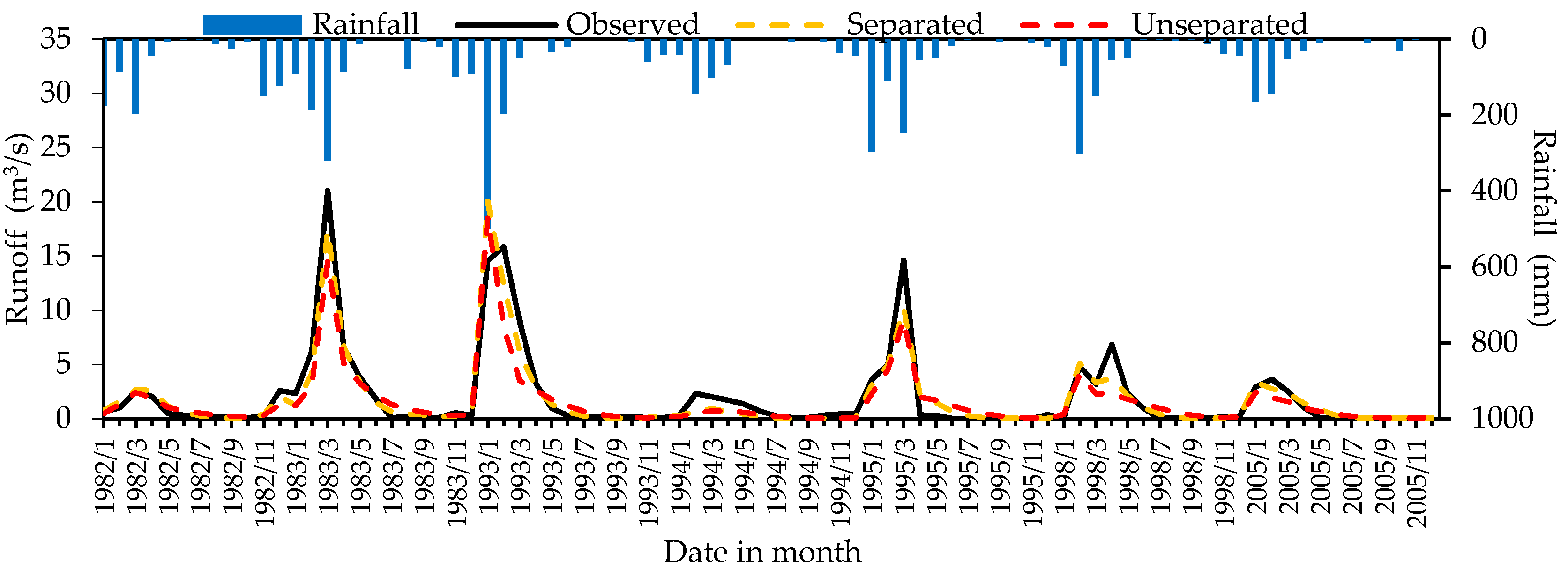
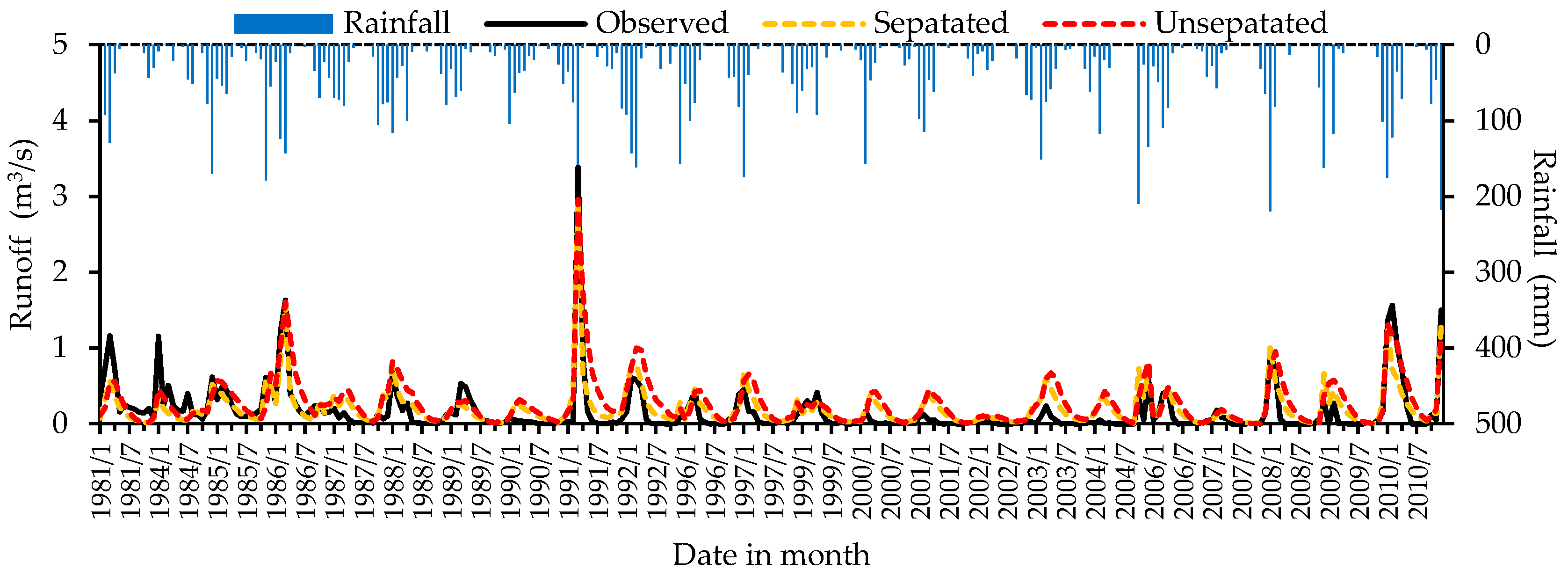
The simulation results of SWAT model with separated calibration were slightly better than those from the unseparated calibration for the wet years, and the hydrograph patterns and peak flows of simulated and observed runoff were generally similar between two calibration methods (Figure 5). In contrast, for the dry years, the goodness-of-fit of the simulated results with separated calibrations was significantly higher than that with the unseparated calibration (Figure 6).
4. Discussion
4.1. Comparison of Sensitive Parameters
There were 8 sensitive parameters in Barrett watershed identified by sensitivity analysis (Figure 4, Table 3). The sensitive parameters of SWAT model in other watersheds of semi-arid regions were also listed in Table 3. They were generally consistent among studies, including CN2, ALPHA_BF, GWQMN, ESCO, and SOL_AWC. CN2 (SCS curve number) and GWQMN (threshold for return flow) were in the top 4 for all studies, and ALPHA_BF (baseflow recession coefficient) and ESCO (soil evaporation) were in the top 4 for all but one study. Parameters relating to soil storage capacity and depth were categorized as sensitive parameters, but the four parameters regulating runoff generation (CN2, GWQMN, ALPHA_BF, and ESCO) were more important in changing model output.
4.2. Formatting of Mathematical Components
Similar to the simulation results of other watersheds with large intra-annual runoff variability [15], SWAT under traditional calibration method did not perform well for both wet and dry periods at Barrett watershed (Table 2), because objective functions such as NSE were sensitive to high flow. To ensure that the objective functions reached acceptable standards for the entire series during the calibration and validation periods, the parameters were adjusted towards a satisfied simulation for the wet years, which lead to poor performance in the dry years.
Six of the eight sensitive parameters (ALPHA_BF, ESCO, CN2, GWQMN, SOL_AWC, and CH_K2) have different values when calibrated to the wet and dry series separately (Table 4). With the traditional method of unseparated wet and dry years, 6 parameters (ALPHA_BF, ESCO, CN2, GWQMN, SOL_AWC, and CH_K2) had values falling between those of the separate wet and dry series, and other two parameters (SOL_K and SOL_Z) were the same between the two methods.
ALPHA_BF was the baseflow alpha factor, which was also known as the baseflow recession constant; it indicates the response of groundwater runoff to supply variation [38] and ranges from 0 to 1. This parameter ranges from 0.1 to 0.3 in regions with slow groundwater response and from 0.9 to 1 in regions with rapid response [39]. Barrett watershed is located in a semi-arid region with low annual precipitation, low vegetation coverage, and poor water conservation capacity, which resulted in slow response of runoff to groundwater . Therefore, the values of ALPHA_BF were less than 0.3 in both the wet and dry years. However, ALPHA_BF was higher in wet years than in dry years, likely because the precipitation in the watershed was higher in wet years than in dry years and resulted in higher groundwater runoff in wet years.
ESCO [40] reflected the evaporation availability of the soil water and had a range of 0–1. This parameter reflects the impact of the soil capillary effect, crust, and cracking on soil water. ESCO modifies the depth distribution of the water content that meets soil evaporation demand. With a decrease in ESCO, the model gains more water that is required by evaporation from the underlying layers, which leads to increased soil evaporation and decreased lateral flow and total runoff. Therefore, the fact that the ESCO value in the dry years was lower than in the wet years was reasonable.
CN2, which has a theoretical range of 35–98, determines the amount of direct surface runoff; the higher the value, the greater the direct runoff. CN2 is a combined function of soil permeability, land use, and antecedent soil moisture conditions [27,41]. The antecedent soil moisture content before rain events was higher in wet years. In addition, the soil infiltration rate decreased with increasing soil water content, and so was higher in dry years than in wet years. In summary, the CN2 value in wet years was higher than that in dry years at Barrett watershed. SWAT adjusts the CN2 for moisture, but our results suggest that the soil adjustment parameter in SWAT did not adequately capture the impact of moisture on the curve number.
GWQMN is the threshold water level of shallow aquifer required for the occurrence of return flow. When the depth of water in the aquifer is greater than or equal to GWQMN, the shallow aquifer will start to transport the groundwater to the main river channel of sub-watershed. GWQMN reflects the sensitivity of the shallow groundwater runoff to precipitation, and the value can greatly impact the discharge from shallow groundwater. The GWQMN value in Barrett watershed was smaller (or easier to produce the return flow) in wet years than in dry years, which was likely due to the fact that the level of groundwater was lower in dry years than in wet years, and it was more difficult to generate groundwater runoff. The large depth of groundwater required to produce runoff from the shallow aquifer in the dry year (200 mm) suggests that SWAT produces little runoff from the shallow aquifer in dry years, and that most runoff in SWAT originates from the direct runoff.
SOL_AWC is the soil effective water content, which indicates the available water for vegetation and reflects the soil’s capacity for water storage [42]. The value of this parameter was higher in dry years than in wet years, which may be caused by the fact that the soil vadose zone was thicker in dry years than in wet years due to the lower water table in dry years, which led to higher water retention capacity.
CH_K2 is the effective hydraulic conductivity of the main channel alluvium [43] and reflects the differences in the characteristics of river beds of different watersheds. The value of this parameter was lower in dry years than in wet years, which indicated that the river channel surface water infiltration capability was lower in dry years than in wet years, though field measurements would be required to validate this conclusion.
SOL_K and SOL_Z remain the same in the wet and dry years. SOL_K is the soil’s saturated hydraulic conductivity [44], which is related to the soil water discharge and hydraulic gradient and can be used to measure the difficulty of water movement in the soil. SOL_Z is the depth between the soil surface and the bottom layer [45].
5. Conclusions
This study analyzed the sensitivity of SWAT model’s process parameters, simulated the monthly runoff by the traditional calibration using the entire data series and the calibration by separating wet and dry years of the watershed, and discussed the differences of the main sensitive parameters of the hydrological processes in the wet and dry years.
(1) When there was a large inter-annual variability of runoff, the SWAT model with the traditional calibration had low simulation efficiency during the dry years and did not meet the performance requirements.
(2) Calibration by separating wet and dry years greatly improved the SWAT model’s simulation efficiency of monthly runoff in the dry years and also improved the simulation results for the wet years and the entire series. This calibration method is worthy of further study and application.
(3) Six main sensitive parameters of SWAT model (ALPHA_BF, CH_K2, CN2, ESCO, GWQMN, and SOL_AWC) were different between the wet and dry years, which indicated that the hydrological conditions or responses in this watershed were different between the wet and dry years. The adjustment highlighted that SWAT does not fully account for the impact of antecedent soil moisture on runoff production and baseflow recession rates in this semi-arid region. SWAT over-predicted direct runoff production from storms that occurred during dry periods, even after adjusting for soil antecedent moisture conditions. This suggests that there are non-linearities in the rainfall-runoff response that are not adequately represented in SWAT, and that SWAT may be capable of simulating discharge during dry years in semi-arid regions, but only after adjusting parameters to greatly reduce runoff generation under conditions of low catchment moisture storage.
Acknowledgments
The study was financially supported by the Science and Technology Major Project of Fujian Province (Grant No. 2015Y4002). The City of San Diego provided data on reservoir inflow. Lara Barrett compiled the input data for the SWAT model.
Author Contributions
Xingwei Chen conceived and designed this study. Xin Gao analyzed the data and drafted the manuscript. All authors contributed to editing the manuscript.
Conflicts of Interest
The authors declare that there is no conflict of interest.
References
- Eckhardt, K.; Arnold, J.G. Automatic calibration of a distributed catchment model. J. Hydrol. 2001, 251, 103–109. [Google Scholar] [CrossRef]
- Wang, Z.G.; Zheng, H.X.; Liu, C.M.; Zhao, W.M. GIS/RS based distributed hydrological modeling 1, model theories and structures. Adv. Water Sci. 2004, 15, 501–505. [Google Scholar]
- Sellami, H.; Vanclooster, M.; Benabdallah, S.; Jeunesse, I.L. Assessment of the SWAT model prediction uncertainty using the GlUE approach a case study of the Chiba Catchment (Tunisia). In Proceedings of the 5th International Conference on Modeling, Simulation and Applied Optimization, Hammamet, Tunisia, 28–30 April 2013; pp. 1–6. [Google Scholar]
- Ahl, R.S.; Woods, S.W.; Zuuring, H.R. Hydrologic calibration and validation of SWAT in a snow-dominated Rocky Mountain watershed, Montana, U.S.A. J. Am. Water Resour. Assoc. 2008, 44, 1411–1430. [Google Scholar] [CrossRef]
- Fontaine, T.A.; Cruickshank, T.S.; Arnold, J.G.; Hotchkiss, R.H. Development of a snowfall–snowmelt routine for mountainous terrain for the soil water assessment tool (SWAT). J. Hydrol. 2002, 262, 209–223. [Google Scholar] [CrossRef]
- Garee, K.; Chen, X.; Bao, A.; Wang, Y.; Meng, F. Hydrological modeling of the upper indus basin: A case study from a high-altitude glacierized catchment Hunza. Water 2017, 9, 17. [Google Scholar] [CrossRef]
- Liu, R.; Xu, F.; Zhang, P.; Yu, W.; Men, C. Identifying non-point source critical source areas based on multi-factors at a basin scale with SWAT. J. Hydrol. 2016, 533, 379–388. [Google Scholar] [CrossRef]
- Vigiak, O.; Malagó, A.; Bouraoui, F.; Vanmaercke, M.; Obreja, F.; Poesen, J.; Habersack, H.; Fehér, J.; Grošelj, S. Modelling sediment fluxes in the danube river basin with SWAT. Sci. Total Environ. 2017, 599–600, 992–1012. [Google Scholar] [CrossRef] [PubMed]
- Li, H.; Sivapalan, M.; Tian, F. Comparative diagnostic analysis of runoff generation processes in Oklahoma Dmip2 basins: The Blue river and the Illinois river. J. Hydrol. 2010, 418–419, 90–109. [Google Scholar] [CrossRef]
- Porretta-brandyk, L.; Chormański, J.; Brandyk, A.; Okruszko, T. Automatic Calibration of the Wetspa Distributed Hydrological Model for Small Lowland Catchments; Springer: Berlin/Heidelberg, Germany, 2011; pp. 43–62. [Google Scholar]
- Legates, D.R.; McCabe, G.J. Evaluating the use of “goodness-of-fit” measures in hydrologic and hydroclimatic model validation. Water Resour. Res. 1999, 35, 233–241. [Google Scholar] [CrossRef]
- White, E.D.; Feyereisen, G.W.; Veith, T.L.; Bosch, D.D. Improving daily water yield estimates in the little river watershed: SWAT adjustments. Trans. ASABE 2009, 52, 69–79. [Google Scholar] [CrossRef]
- Muleta, M.K. Improving model performance using season-based evaluation. J. Hydrol. Eng. 2012, 17, 191–200. [Google Scholar] [CrossRef]
- Lévesque, É.; Anctil, F.; van Griensven, A.; Beauchamp, N. Evaluation of streamflow simulation by SWAT model for two small watersheds under snowmelt and rainfall. Hydrol. Sci. J. 2008, 53, 961–976. [Google Scholar] [CrossRef]
- Zhang, D.; Chen, X.; Yao, H.; Lin, B. Improved calibration scheme of SWAT by separating wet and dry seasons. Ecol. Model. 2015, 301, 54–61. [Google Scholar] [CrossRef]
- Singh, V.V.; Sharma, A. Modelling of runoff response in a semi-arid coastal watershed using SWAT. Int. J. Eng. Res. Appl. 2015, 5, 50–57. [Google Scholar]
- Zettam, A.; Taleb, A.; Sauvage, S.; Boithias, L.; Belaidi, N.; Sánchez-pérez, J.M. Modelling hydrology and sediment transport in a semi-arid and anthropized catchment using the SWAT model: The case of the Tafna river (northwest Algeria). Water 2017, 9, 216. [Google Scholar] [CrossRef]
- Jahanshahi, A.; Golshan, M.; Afzali, A. Simulation of the catchments hydrological processes in arid, semi-arid and semi-humid areas. Desert 2017, 22, 1–10. [Google Scholar]
- Chang, C.H.; Cai, L.Y.; Lin, T.F.; Chung, C.L.; Linden, L.V.D.; Burch, M. Assessment of the impacts of climate change on the water quality of a small deep reservoir in a humid-subtropical climatic region. Water 2015, 7, 1687–1711. [Google Scholar] [CrossRef]
- Cheng, L.; Xu, Z.X.; Luo, R.; Mi, Y.J. SWAT application in arid and semi-arid region: A case study in the Kuye river basin. Geogr. Res. 2009, 27, 96–102. [Google Scholar]
- Mosbahi, M.; Benabdallah, S.; Boussema, M.R. Hydrological Modeling in a semi-arid catchment using SWAT model. J. Environ. Sci. Eng. 2011, 5, 1695–1701. [Google Scholar]
- Niraula, R.; Norman, L.M.; Meixner, T.; Callegary, J.B. Multi-gauge calibration for modeling the semi-arid Santa Cruz watershed in Arizona-Mexico border area using SWAT. Air Soil Water Res. 2012, 5, 41. [Google Scholar] [CrossRef]
- Hill, J. Dry rivers, Dry rivers, dammed rivers and floods: An early history of the struggle between droughts and floods in San Diego. J. San Diego Hist. 2002, 48, 48–59. [Google Scholar]
- Herzog, L.A. Planning the International Border Metropolis: Trans-Boundary Policy Options in the San Diego-Tijuana Region; Center for U.S.-Mexican Studies, University of California: San Diego, CA, USA, 1986. [Google Scholar]
- Kottek, M.; Grieser, J.; Beck, C.; Rudolf, B.; Rubel, F. World map of the köppen-geiger climate classification updated. Meteorol. Z. 2006, 15, 259–263. [Google Scholar] [CrossRef]
- Arnold, J.G.; Srinivasan, R.; Muttiah, R.S.; Williams, J.R. Large area hydrologic modeling and assessment part I: Model development. J. Am. Water Resour. Assoc. 1998, 34, 91–101. [Google Scholar] [CrossRef]
- Boughton, W.C. A review of the USDA SCS curve number method. Aust. J. Soil Res. 1989, 27, 511–523. [Google Scholar] [CrossRef]
- Green, W.H.; Ampt, G.A. Studies on soil phyics. J. Agric. Sci. 1911, 4, 1–24. [Google Scholar] [CrossRef]
- Williams, J.R. Flood routing with variable travel time or variable storage coefficients. Trans. ASABE 1969, 12, 100–103. [Google Scholar] [CrossRef]
- Gill, M.A. Flood routing by the muskingum method. J. Hydrol. 1978, 36, 353–363. [Google Scholar] [CrossRef]
- Thornton, P.E.; Thornton, M.M.; Mayer, B.W.; Wilhelmi, N.; Wei, Y.; Devarakonda, R.; Cook, R.B. Daymet: Daily Surface Weather Data on a 1-km Grid for North America, Version 2; Oak Ridge National Laboratory Distributed Active Archive Center: Oak Ridge, TN, USA, 2014. [Google Scholar]
- Griensven, A.V.; Meixner, T.; Grunwald, S.; Bishop, T.; Diluzio, M.; Srinivasan, R. A global sensitivity analysis tool for the parameters of multi-variable catchment models. J. Hydrol. 2006, 324, 10–23. [Google Scholar] [CrossRef]
- Mckay, M.D.; Beckman, R.J.; Conover, W.J. A comparison of three methods for selecting values of input variables in the analysis of output from a computer code. Technometrics 2000, 21, 239–245. [Google Scholar] [CrossRef]
- Morris, M.D. Factorial sampling plans for preliminary computational experiments. Technometrics 1991, 33, 161–174. [Google Scholar] [CrossRef]
- Lenhart, T.; Eckhardt, K.; Fohrer, N.; Frede, H.G. Comparison of two different approaches of sensitivity analysis. Phys. Chem. Earth 2002, 27, 645–654. [Google Scholar] [CrossRef]
- Abbaspour, K.C.; Vejdani, M.; Haghighat, S. SWAT-CUP Calibration and uncertainty programs for SWAT. In Proceedings of the International Congress on Modelling and Simulation, Land Water and Environmental Management Integrated Systems for Sustainability MODISM, Christchurch, New Zealand, 2007. [Google Scholar]
- Moriasi, D.N.; Arnold, J.G.; Liew, M.W.; Bingner, R.L.; Harmel, R.D.; Veith, T.L. Model evaluation guidelines for systematic quantification of accuracy in watershed simulations. Trans. ASABE 2007, 50, 885–900. [Google Scholar] [CrossRef]
- Smedema, L.K.; Rycroft, D.W. Land Drainage: Land drainage: Planning and design of agricultural systems. Soil Sci. 1983, 139, 378. [Google Scholar]
- Neitsch, S.L.; Arnold, J.G.; Kiniry, J.R.; Williams, J.R. Soil and Water Assessment Tool Theoretical Documentation Version 2009; Texas Water Resources Institute: College Station, TX, USA, 2011. [Google Scholar]
- Bodner, G.; Loiskandl, W.; Kaul, H.P. Cover crop evapotranspiration under semi-arid conditions using FAO dual crop coefficient method with water stress compensation. Agric. Water Manag. 2007, 93, 85–98. [Google Scholar] [CrossRef]
- Bosznay, M. Generalization of SCS curve number method. J. Irrig. Drain. Eng. 1989, 115, 139–144. [Google Scholar] [CrossRef]
- Kern, J.S. Geographic patterns of soil water-holding capacity in the contiguous United States. Soil Sci. Soc. Am. J. 1995, 59, 1126–1133. [Google Scholar] [CrossRef]
- Genereux, D.P.; Leahy, S.; Mitasova, H.; Kennedy, C.D.; Corbett, D.R. Spatial and temporal variability of streambed hydraulic conductivity in west Bear creek, North Carolina, USA. J. Hydrol. 2008, 358, 332–353. [Google Scholar] [CrossRef]
- Wilson, G.V.; Jardine, P.M.; Alfonsi, J.M. Spatial variability of saturated hydraulic conductivity of the subsoil of two forested watersheds. Soil Sci. Soc. Am. J. 1989, 53, 679–685. [Google Scholar] [CrossRef]
- Wong, M.T.F.; Oliver, Y.M.; Robertson, M.J. Gamma-radiometric assessment of soil depth across a landscape not measurable using electromagnetic surveys. Soil Sci. Soc. Am. J. 2017, 9, 1261–1267. [Google Scholar] [CrossRef]
Figure 1.
Location and station distribution of the Barrett watershed.

Figure 2.
Distribution of the wet and dry years in Barrett watershed (1981–2010).

Figure 3.
Flow diagram of the calibration method for separate wet and dry years.

Figure 4.
Results of the sensitivity analysis in Barrett watershed.

Figure 5.
Comparison between simulated and measured monthly runoff in the wet years.

Figure 6.
Comparison between simulated and measured monthly runoff in the dry years.


Table 1.
Sensitivity ranking.
| Rank | Index | Sensitivity |
|---|---|---|
| I | 0 ≤ Si < 0.0.5 | Small to negligible |
| II | 0.05 ≤ Si < 0.20 | Medium |
| III | 0.2 ≤ Si < 1 | High |
| IV | Si ≥ 1 | Very high |
Table 2.
Comparison of NSE, R2, and RE between the calibration with separated and unseparated method.
Table 2.
Comparison of NSE, R2, and RE between the calibration with separated and unseparated method.
| Model | Series | Duration | R2 | RE (%) | NSE |
|---|---|---|---|---|---|
| Unseparated | Wet series | Calibration | 0.89 | −17.87 | 0.84 |
| Validation | 0.80 | −12.86 | 0.66 | ||
| Dry series | Calibration | 0.64 | 41.57 | 0.56 | |
| Validation | 0.60 | 108.42 | 0.34 | ||
| Entire series | Calibration | 0.90 | −7.48 | 0.86 | |
| Validation | 0.78 | 32.44 | 0.71 | ||
| Separated | Wet series | Calibration | 0.91 | −9.64 | 0.90 |
| Validation | 0.87 | −2.76 | 0.85 | ||
| Dry series | Calibration | 0.81 | 1.78 | 0.80 | |
| Validation | 0.68 | 66.29 | 0.60 | ||
| Entire series | Calibration | 0.92 | −7.65 | 0.91 | |
| Validation | 0.88 | 23.13 | 0.86 |
Table 3.
Sensitivity ranking of SWAT parameters for 4 studies in different semi-arid watersheds.
| Sensitive Parameters | Barrett | Sarrath | Santa Cruz | Saurashtra | Rank (4 Studies) | Rank (3 Studies) |
|---|---|---|---|---|---|---|
| (America) | (Algeria) [21] | (Mexico) [22] | (India) [16] | |||
| ALPHA_BF | 1 | - | 4 | 1 | - | 1 (sum = 6) |
| CN2 | 3 | 1 | 1 | 3 | 1 (sum = 8) | 2 (sum = 7) |
| CH_K2 | 8 | - | 5 | 4 | - | 5 (sum = 17) |
| CH_N2 | - | - | - | 5 | - | - |
| ESCO | 2 | 2 | 2 | 7 | 3 (sum = 13) | 4 (sum = 11) |
| GWQMN | - | - | - | 6 | - | - |
| GWQMN | 4 | 3 | 3 | 2 | 2 (sum = 12) | 3 (sum = 9) |
| SLSUBBSN | - | 4 | - | - | - | - |
| SOL_AWC | 7 | - | 6 | 8 | - | 6 (sum = 21) |
| SOL_K | 5 | - | - | 9 | - | - |
| SOL_Z | 6 | - | 7 | 10 | - | - |
Note: Rank (4 studies) is based on the sum of ranks for all four studies, and Rank (3 studies) is the sum of ranks excluding Sarrath.
Table 4.
Values of the parameters determined in the calibration.
| Parameter | Process | Unit | Default Range | Unseparated | Separated | |
|---|---|---|---|---|---|---|
| Wet Years | Dry Years | |||||
| ALPHA_BF.gw | Groundwater | days | 0–1 | 0.17 | 0.20 | 0.08 |
| ESCO.hru | Evaporation | - | 0–1 | 0.20 | 0.37 | 0.18 |
| CN2.mgt | Surface runoff | - | 35-98 | 41.89–65.32 | 43.37–67.62 | 38.35–59.80 |
| GWQMN.gw | Groundwater | mm | 0–5000 | 30.00 | 20.00 | 200.00 |
| SOL_K.sol | Soil water | mm/h | 0–2000 | 0–4.00 | 0–4.00 | 0–4.00 |
| SOL_Z.sol | Soil water | mm | 0–3500 | 0.55 | 0.55 | 0.55 |
| SOL_AWC.sol | Soil water | mm/mm | 0–1 | 0.17–0.27 | 0.17–0.27 | 0.18–0.28 |
| CH_K2.rte | Channel water | mm/h | −0.01–500 | 70.00 | 80.00 | 22.00 |
© 2018 by the authors. Licensee MDPI, Basel, Switzerland. This article is an open access article distributed under the terms and conditions of the Creative Commons Attribution (CC BY) license (http://creativecommons.org/licenses/by/4.0/).
Share and Cite
MDPI and ACS Style
Gao, X.; Chen, X.; Biggs, T.W.; Yao, H. Separating Wet and Dry Years to Improve Calibration of SWAT in Barrett Watershed, Southern California. Water 2018, 10, 274. https://doi.org/10.3390/w10030274
AMA Style
Gao X, Chen X, Biggs TW, Yao H. Separating Wet and Dry Years to Improve Calibration of SWAT in Barrett Watershed, Southern California. Water. 2018; 10(3):274. https://doi.org/10.3390/w10030274
Chicago/Turabian StyleGao, Xin, Xingwei Chen, Trent W. Biggs, and Huaxia Yao. 2018. "Separating Wet and Dry Years to Improve Calibration of SWAT in Barrett Watershed, Southern California" Water 10, no. 3: 274. https://doi.org/10.3390/w10030274
Note that from the first issue of 2016, this journal uses article numbers instead of page numbers. See further details here.