Effects of Water Level Increase on Phytoplankton Assemblages in a Drinking Water Reservoir
by
Yangdong Pan
1,2, 
Shijun Guo
1,3,
Yuying Li
1,3,*,
Wei Yin
1,4,
Pengcheng Qi
1,3,
Jianwei Shi
1,5,
Lanqun Hu
1,5,
Bing Li
1,3,
Shengge Bi
1,3 and
Jingya Zhu
1,3 1
Collaborative Innovation Center of Water Security for Water Source Region of Middle Route Project of South-North Water Diversion of Henan Province, Nanyang Normal University, Nanyang 473061, Henan, China
2
Department of Environmental Science and Management, Portland State University, Portland, OR 97207, USA
3
Key Laboratory of Ecological Security for Water Source Region of Middle Route Project of South-North Water Diversion of Henan Province, College of Agricultural Engineering, Nanyang Normal University, Nanyang 473061, Henan, China
4
Changjiang Water Resources Protection Institute, Changjiang Water Resources Commission, Wuhan 430051, Hubei, China
5
Emergency Centre for Environmental Monitoring of the Canal Head of Middle Route Project of South-North Water Division, Xichuan 474475, Henan, China
*
Author to whom correspondence should be addressed.
Water 2018, 10(3), 256; https://doi.org/10.3390/w10030256
Submission received: 18 January 2018
/
Revised: 25 February 2018
/
Accepted: 27 February 2018
/
Published: 2 March 2018
(This article belongs to the Special Issue Biological Communities Respond to Multiple Human-Induced Aquatic Environment Change)
Abstract
:Excessive water level fluctuation may affect physico-chemical characteristics, and consequently ecosystem function, in lakes and reservoirs. In this study, we assessed the changes of phytoplankton assemblages in response to water level increase in the Danjiangkou Reservoir, one of the largest drinking water reservoirs in Asia. The water level increased from a low of 137 m to 161 m in 2014 as a part of the South–North Water Diversion Project. Phytoplankton assemblages were sampled four times per year before, during and after the water level increase, at 10 sites. Environmental variables such as total nitrogen as well as phytoplankton biomass decreased after the water level increase. Non-metric multi-dimensional scaling analysis indicated that before the water level increase, phytoplankton assemblages showed distinct seasonal variation with diatom dominance in both early and late seasons while such seasonal variation was much less evident after the water level increase. Month and year (before and after) explained 13% and 6% of variance in phytoplankton assemblages (PERMANOVA, p < 0.001) respectively, and phytoplankton assemblages were significantly different before and after the water level increase. Both chlorophytes and cyanobacteria became more abundant in 2015. Phytoplankton compositional change may largely reflect the environmental changes, such as hydrodynamics mediated by the water level increase.
1. Introduction
Ecological impacts of excessive water level fluctuation (WLF) in both lakes and reservoirs have received increasing attention from both ecologists and water resource managers [1,2,3,4,5]. The water level does fluctuate naturally, but an increase in global climate variability (e.g., precipitation) is expected to result in more extreme hydrological events, such as extended droughts and flooding. Consequently, both intensity and frequency of excessive WLF in lakes and reservoirs will increase, which will adversely affect water supply, food security, and aquatic ecosystems [6,7,8]. Excessive WLF may affect both physical and chemical characteristics of lakes and reservoirs including quantity and quality of littoral zone habitat, light, thermal stratification/mixing, and internal nutrients and consequently affect freshwater ecosystem structure and function [8,9,10,11]. For instance, water level fluctuation caused significant reduction of benthic algal productivity and macroinvertebrate diversity in littoral zones [8]. The littoral zones, a critical ecotone for biodiversity, habitats, primary productivity, and material exchanges between aquatic and terrestrial ecosystems [10], have been the focus of many ecological studies on the impacts of WLF, particularly in shallow lakes and wetlands, two of the most vulnerable ecosystems to WLF [9]. The studies on the ecological impacts of WLF on deep drinking water reservoirs are still relatively limited [8].
The intensity and frequency of WLF in deep reservoirs in response to anthropogenic demands—such as drinking water, hydropower generation, or irrigation—may be much higher than that in natural lakes, particularly under the projected extreme climate change scenarios [8]. For instance, the maximum amplitude of WLF in Lake Shasta, a reservoir in California (USA), reached as high as 47 m between 1991 and 1993 compared to less than 3 m in some natural lakes [2]. In deep lakes and reservoirs, excessive WLF can also potentially disrupt thermal structure, alter mixing regimes and internal nutrient cycles, and consequently increase the likelihood for algal blooms [1,5,12,13]. For instance, due to an extended drought, the water level in Lake Burragorang—a drinking water reservoir in Australia—dropped 25 m. Vilhena et al. used both hydrodynamic and ecological models to demonstrate that large river inflow could disrupt thermal stratification when the lake water level was extremely low, release dissolved nutrients from the hypolimnion, and result in a subsequent Microcystis bloom. It is expected that climate change will likely aggravate the negative impacts of WLF on drinking water reservoirs, particularly in the regions with high population growth, urbanization, and rapid economic development [8]. Better understanding of the impacts of excessive WLF on drinking water reservoirs, particularly on water quality, will help water resource managers design optimal operation and develop mitigation plans for climate change.
Existing water infrastructure are often not designed to cope with the impacts of climate change [1,7]. China’s South–North Water Diversion Project is a part of its national strategy to adapt and mitigate climate change and meet a rapidly increasing demand for drink water and irrigation. This multi-billion dollar project aims to divert abundant water resource from the Yangtze River and its tributaries in the south to the water-stressed north China plain. The Danjiangkou Reservoir, one of the largest drinking water reservoirs in Asia, is the source water for the middle route of the South–North Water Diversion Project [14]. To prepare for the water diversion, the water level at the reservoir was increased after the original dam height was raised to increase its water storage capacity. This large-scale water-level manipulation in a reservoir may provide a valuable natural experiment on the ecological effects of WLF and future best management practices. In this study, we tested if the water level increase had significant effects on phytoplankton assemblages in the reservoir before and after the water level increase. Most of the studies on WLF focus on the effects of decreasing water levels on aquatic ecosystems. The studies on the ecological impacts of excessive WLF on drinking reservoirs are often hampered by limited long-term monitoring data of physio-chemical and particular biological parameters. Under the projected extreme climate change scenarios, it is expected that drinking water reservoirs including Danjiangkou may experience higher intensity and frequency of water level fluctuation. Both design and operation of water infrastructure such as drinking reservoirs traditionally focus more on water quantity. A better operation and management practice should include water quality as one of the management priorities, particularly because several excessive WLF events resulted in harmful algal blooms [1,5,12,13]. Characterizing phytoplankton assemblages with relation to water level changes will help develop a long-term ecological monitoring system for drinking water quality in the future. We expected that the increase of the water level in the reservoir would affect both hydrodynamics and nutrients associated with newly flooded lands and consequently both spatial and temporal variation of phytoplankton assemblages in the reservoir.
2. Materials and Methods
2.1. Study Area
The Danjiangkou Reservoir, located in central China (32°36′–33°48′ N; 110°59′–111°49′ E), is one of the largest reservoirs in Asia (Figure 1). The dam was initially constructed on the upper reach of the Han River, one of the largest tributaries of the Yangtze River, in 1973. As one of China’s three trans-basin water transfer projects [14], the reservoir’s water storage capacity was further expanded by increasing the dam height from 162.0 m to 176.6 m above sea level in 2013 (Table A1). The reservoir surface area was increased from 745 km2 at the normal water level of 157 m to 1050 km2 at the normal water level of 170 m with a maximum water depth of approximately 80 m. The Han and Dan rivers, two major tributaries, flow into the reservoir and form two major arms, i.e., the Han Reservoir (DRH) and the Dan Reservoir (DRD), separated by the provincial border line between Hubei and Henan provinces (Figure 1). The reservoir is approximately isothermal from November to March and thermal stratification typically starts in April [15].
The climate in the region is characterized as a subtropical monsoon with hot and humid summers and mild winters. The mean annual temperature is 15.7 °C, with a monthly average of 27.3 °C in July and 4.2 °C in January. Approximately 80% the annual precipitation of 749.3 mm occurs between May and September (wet season) [16]. With >200 tributaries flowing into the reservoir, the watershed includes an area of approximately 95,200 km2. The elevation in the watershed varies between 201 and 3500 m a.s.l. The watershed is dominated by forests (>75%) with major vegetation types varied from deciduous broadleaves, conifers, to alpine shrub meadows along an elevational gradient [17]. Approximately 15% of the watershed, primarily in the area with a gentle slope below an elevation of 1000 m, is agricultural land with corn and wheat as the two major crops. The top 30 cm of soil consists of 48% clay, 41% silt, and 11% sand [18].
2.2. Field Sampling and Sampling Time
A total of 10 sites were selected for assessing spatial variability of phytoplankton assemblages in the reservoir (Figure 1b) and each site was sampled in January, May, July, and October during 2014–2016 for assessing both seasonal and year-to-year variability. The three years corresponding to the three phases of the water level changes. The number of sites, skewed more toward the Dan River arm (DRD) (n = 7) than the Han River arm (n = 3), reflect the spatial variability within each arm of the reservoir. The Han River arm, confined by narrow rocky canyons, is much more river-like with relatively fast flow while the Dan River arm includes both upper riverine section and a much more lentic pelagic zone below the confluence of the Dan and Guan rivers (Figure 1b). At each site, a sample of 5 L of water for phytoplankton assemblage was collected at 50 cm below the water surface using a Van Dorn sampler and was preserved immediately with 1% Lugol’s solution in January, May, July, and October during the period of 2014–2016. Water temperature (T), pH, conductivity (CD), and dissolved oxygen (DO) were measured in situ using a YSI multi-probe (YSI 6920, USA). Transparency was measured using a Secchi disk (SD).
2.3. Laboratory Analysis
Each phytoplankton sample was concentrated to 30 mL using a glass sedimentation utensil for 48 h. Phytoplankton was counted in a Fuchs–Rosental counting chamber of 0.1 mL under a microscope (Nikon E200, Kanagawa ken, Japan) at 400× magnification. A minimum of 500 algal units were identified to the lowest taxonomic level possible and enumerated for characterizing overall algal assemblages [19,20,21]. Biovolume of each taxon was calculated based on measured morphometric characteristics (diameter, length, and width). Conversion to biomass was based on 1 mm3 of algal volume equals 1 mg of fresh weight biomass. For diatom species identification, samples were processed with acid reagents [19].
Total phosphorus (TP) and total nitrogen (TN) were analyzed based on the standard methods of Chinese Ministry of Environmental Protection [22,23]. TP was analyzed using ammonium molybdate spectrophotometric method while TN was analyzed using alkaline potassium persulfate digestion UV spectrophotometric method. Chemical oxygen demand (COD) was analyzed with the potassium dichromate method.
2.4. Data Analysis
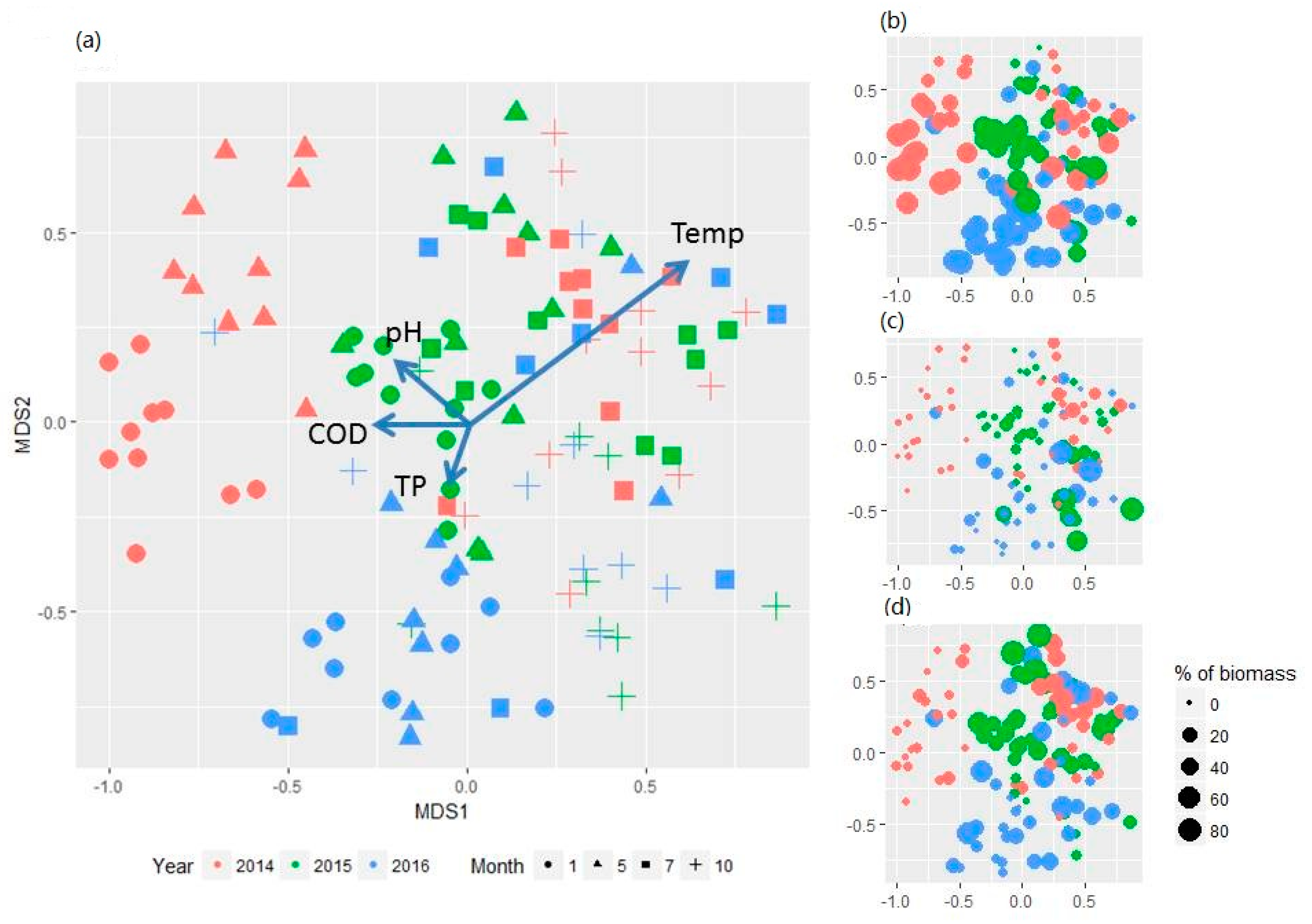
To summarize both spatial and temporal variation of phytoplankton assemblages in the reservoir, we performed non-metric multidimensional scaling (NMDS) with Bray–Curtis dissimilarity index [24]. Algal data as relative abundance of total algal biomass (n = 118, taxa = 193) were square-root transformed to dampen the impacts of dominant taxa on the ordination analysis. The NMDS was run 20 times each with a random starting configuration. The final NMDS dimension was selected based on the lowest stress value among the best solutions. The effects of the reservoir arms (DRH vs. DRD), year (before vs. after water-level increase), and month on phytoplankton assemblages were assessed using permutational multivariate analysis of variance (PERMANOVA, ‘adonis’ function in ‘Vegan’ R package [25]) with repeated measures (month), a non-parametric multivariate statistical test [26]. PERMANOVAs were then conducted for each sampling month with Bonferroni’s correction. Prior to the PERMANOVA tests, the homogeneity of multivariate dispersions among the groups was assessed with Bray–Curtis dissimilarity measure using the ‘betadisper’ function in ‘vegan’ of R package [25]. The test for the homogeneity of multivariate dispersions (Anderson 2006) is a multivariate analogue to Levene’s test [27]. In addition, the phytoplankton assemblage distribution patterns captured by the NMDS were also related with measured environmental variables using ‘envfit’ function in ‘Vegan’ R package [25]. This function fits explanatory variables in the ordination space defined by the species data (i.e., NMDS plot). The importance of each vector was assessed using a squared correlation coefficient (R2). Finally, to characterize what taxa were largely responsible for the assemblage-level changes before, during vs. after water-level increase, the indicator taxa for each year were identified following the methods by Dufrene & Legendre (1997). An indicator value of a species for a year was the product of the relative abundance and the relative frequency of the taxa in the year. The statistical significance of the indicator value was then tested using a permutation test (999 permutations). All analyses were performed using R [28] and an R packages of ‘vegan’ [25] and ‘labdsv’. The datasets generated and/or analyzed during the current study are available from the corresponding author on reasonable request.
3. Results
3.1. Changes of Water Level and Water Quality
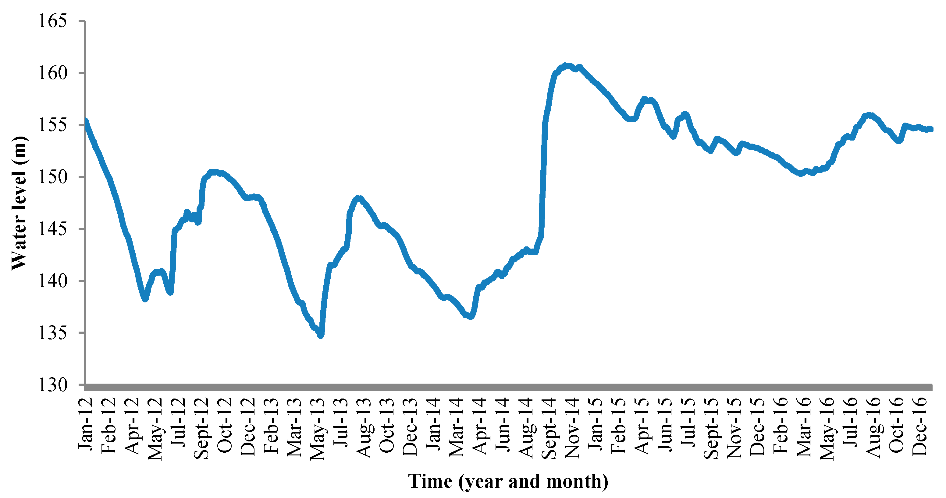
Mean annual water level changed from 144 m (2012–2013) to 154 m (2015–2016) in the Danjiangkou Reservoir (Figure 2, Table A1). Between April and December 2014, the water level increased from 137 m to 161 m, an increase of 24 m (mean = 10 cm/day). From April to October, the water level increased as a part of seasonal variation while from October to December, the water level continued to increase as a part of the water transfer project, which started to release water to the distributional canals on 12 December 2014. The water levels showed pronounced wet and dry seasonal cycles in 2012 and 2013. The annual variations were 17 and 13 m, respectively. After the water transfer project started, annual variation decreased substantially (7 m in 2015 and 6 m in 2016) with no distinct wet and dry seasonal cycles.
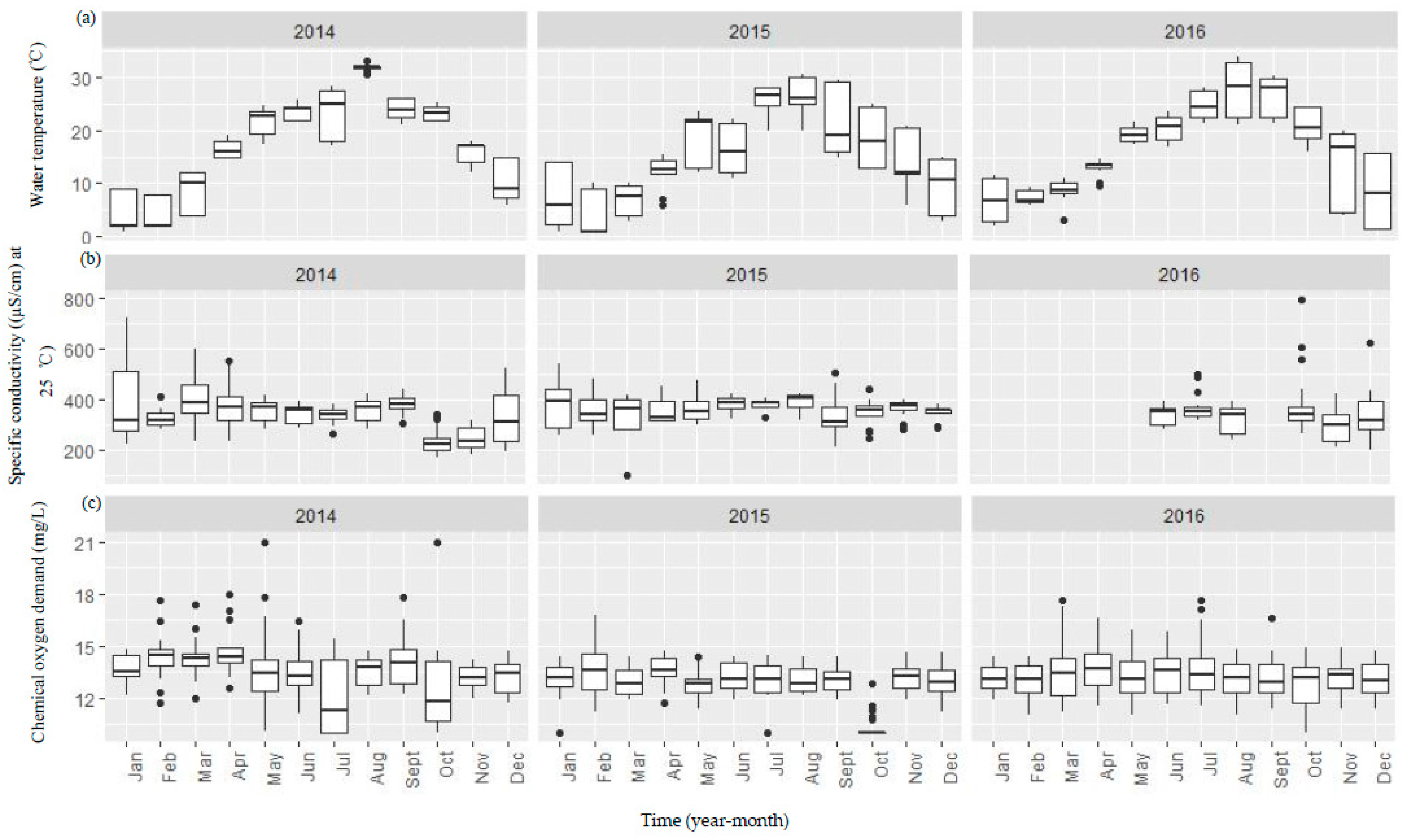
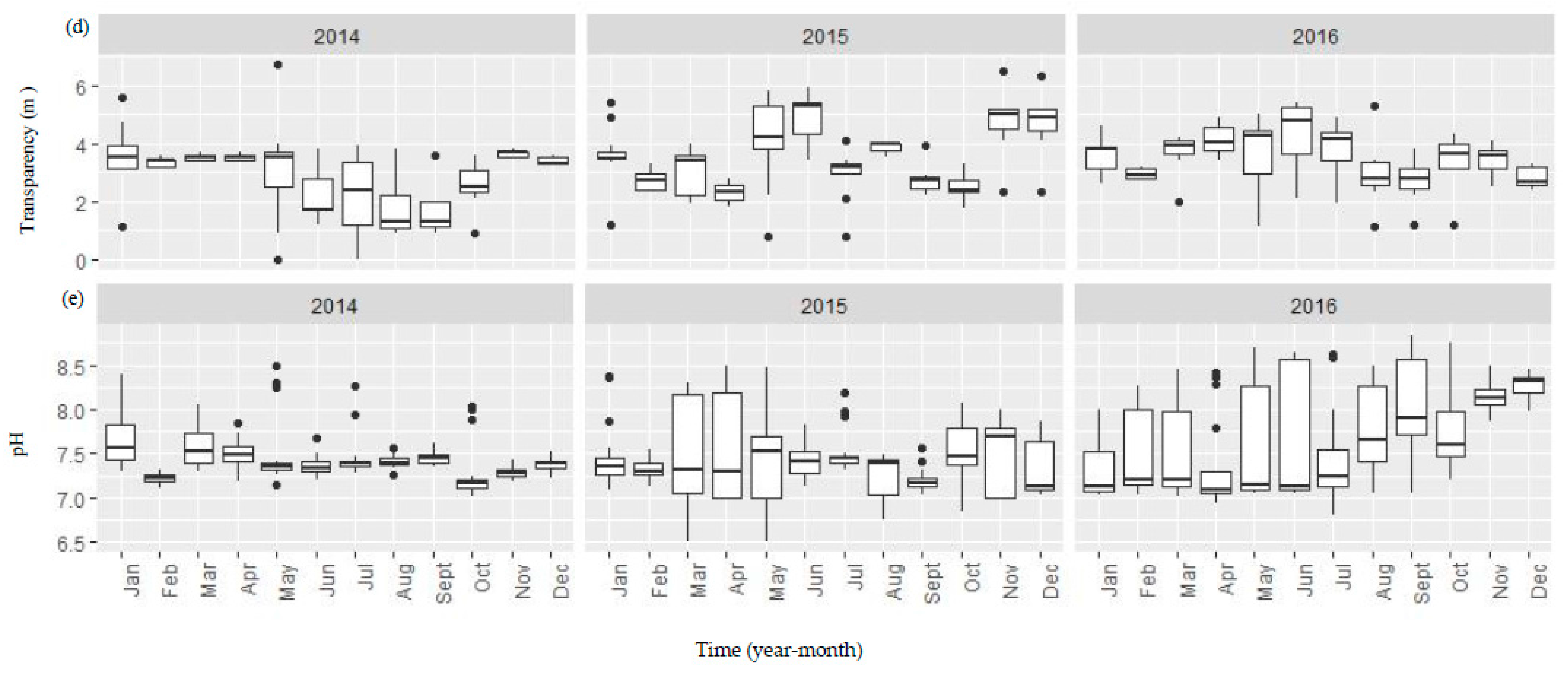
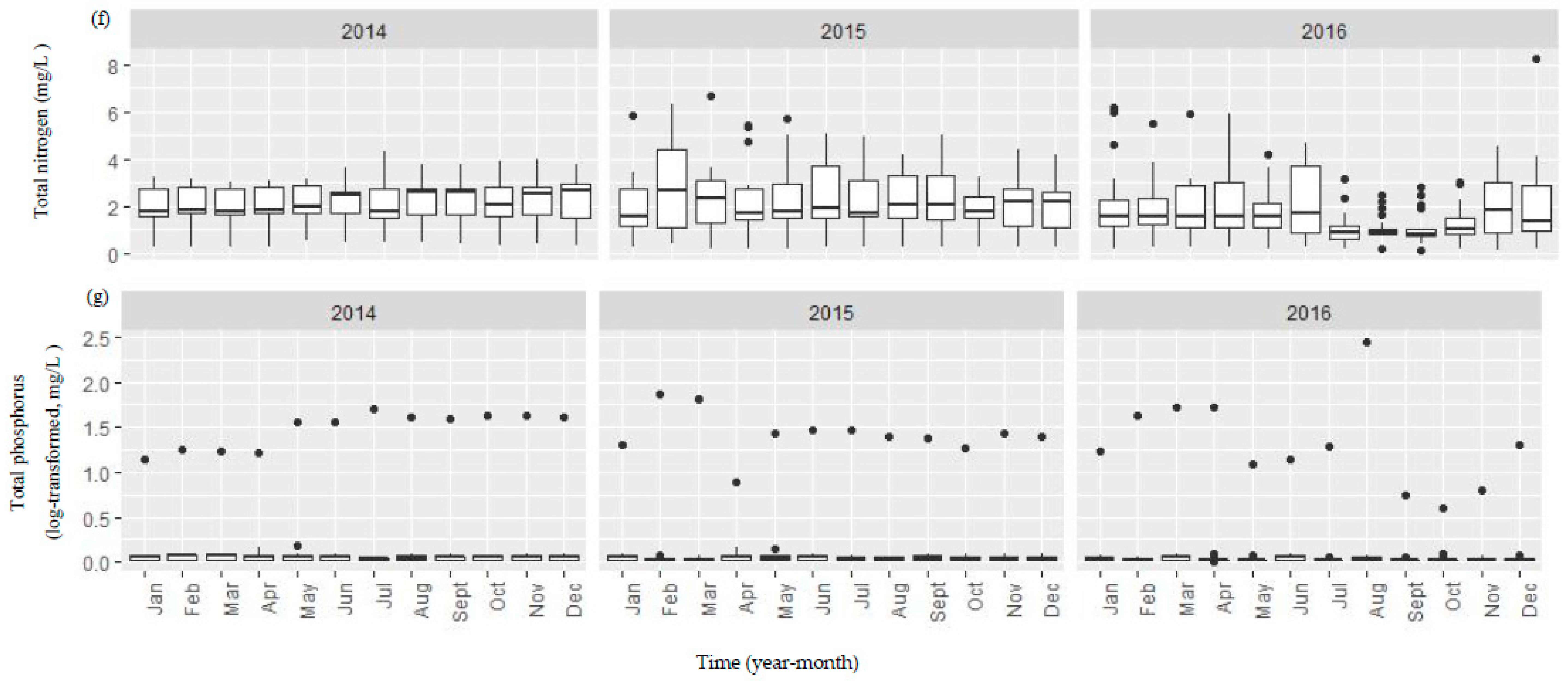
Water in the reservoir in general had high conductivity, low to moderate nutrients, and high water transparency (Figure A1). Water temperature showed similar seasonal variation before, during and after the water level increase. Water quality variables did not show consistent changes before and after the water level increase (Figure A1). Median specific conductivity increased from 336.5 µS/cm in 2014 to 368.5 µS/cm and 342.0 µS/cm in 2015 and 2016, respectively while both median TN and TP concentrations decreased (TN: 2.21 mg/L in 2014, 1.90 mg/L in 2015 and 1.21 mg/L in 2016; TP: 0.05 mg/L in 2014, 0.03 mg/L in 2015, and 0.02 mg/L in 2016). Monthly spatial variation of TN was higher in both 2015 and 2016 than in 2014. Median water transparency remained high (>3.3 m) before and after the water level increase. Median pH was 7.38, 7.43, and 7.33 while median COD was 13.60, 12.95, and 13.20 mg/L before, during, and after the water level increase.
3.2. Changes of Phytoplankton Assemblages in Relation to Environmental Variables
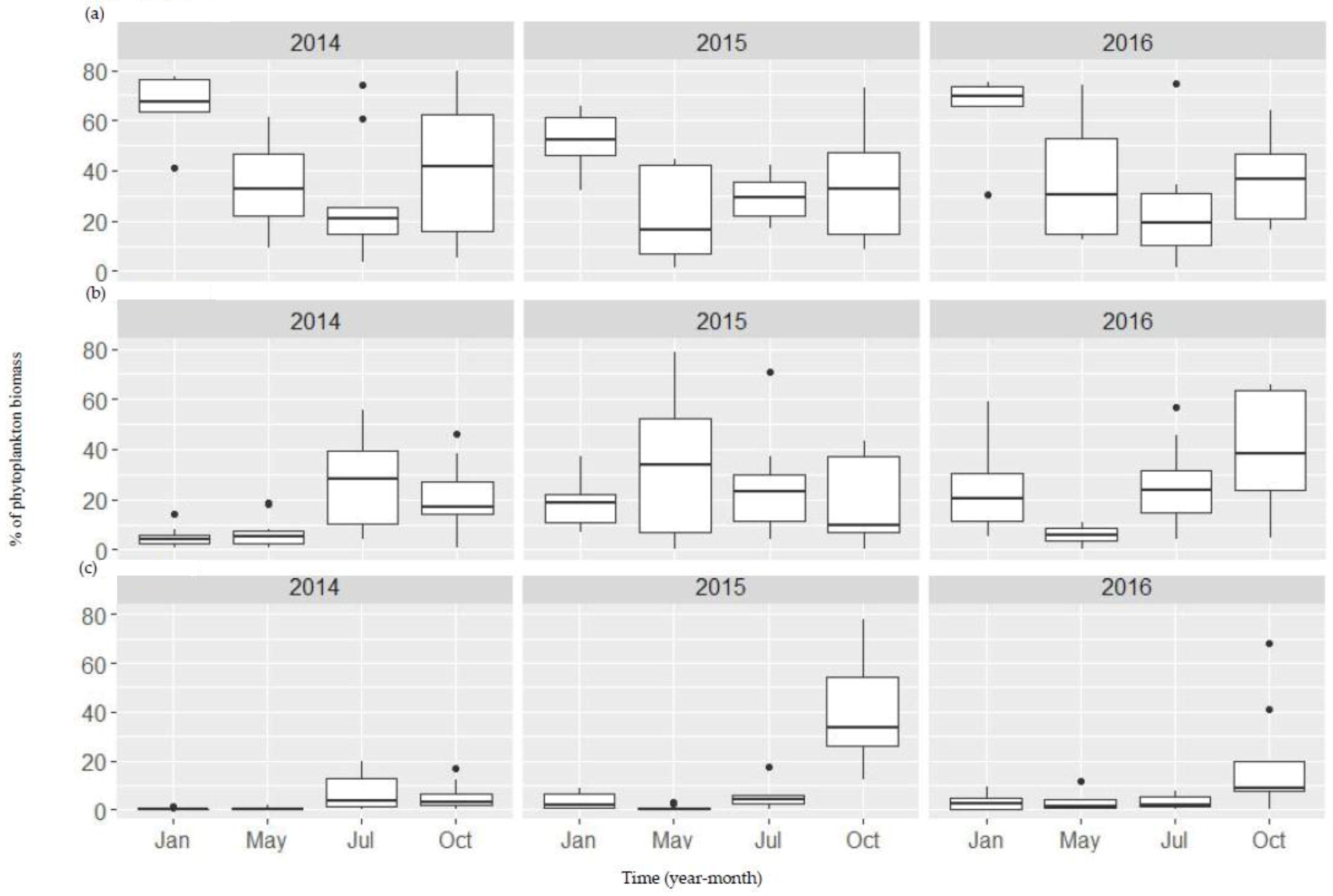
Phytoplankton assemblages changed seasonally before water level increase and year-to-year before and after water level changes (Figure 3). The results of PERMANOVA with repeated measures show that month and year (before, during, and after) as factors explained 13% and 6% of variance in phytoplankton assemblages (p < 0.001 for both factors), respectively, while spatial variation between the two reservoir arms only explained 1% of variance in phytoplankton assemblages. Median phytoplankton biomass in 2014 was 7.4 mg/L and then decreased to 4.9 mg/L and 2.3 mg/L in 2015 and 2016, respectively (Figure A2). PERMANOVA of phytoplankton assemblages for each month indicated that phytoplankton assemblages were significantly different before, during, and after the water level increase for each sampling month (p < 0.001) (Table A2). Before the water level increase, diatoms in both dominance and species composition shifted from a cold and dry season (January and May) to a warm and wet season (July and October) along the first NMDS axis (Figure 3 and Figure A3). In 2014, median diatom levels were highest at 70% of phytoplankton biomass in January and dominated by Cyclotella sp. (30.74%) and Aulacoseira granulata (Ehr.) Simonsen (30.66%) (Figure A3a, Table A3). Dominance of diatoms continued to decline in May and reached its lowest of 20% in July as median chlorophytes (e.g., Eudorina sp.) reached 30% (except for two sites) (Figure 3b). Diatoms became dominant again in October but mainly by Cymbella sp. (14.2%), Synedra sp. (14.0%), and Cyclotella sp. (13.0%) (Figure A3a, Table A3).
Most noticeable changes after the water level increase were that the seasonal differences in phytoplankton assemblages between the dry/cold and warm/wet seasons in 2015 and 2016 became much less evident than in 2014 (Figure 3a). Median chlorophyte relative abundance increased from 8.5% in 2014 to 19.7% and 21.1% in 2015 and 2016, an increase of 57% and 60%, respectively. Chlorophytes were abundant in the early season (May) in 2015, particularly at the sites XJD, BS, and LHK where relative abundance was >80% (Figure A3b). Overall cyanobacteria was relatively low in abundance in 2014 with the highest of 17% at site KX but increased in median abundance to 40% in October 2015 (Figure A3c). At sites TZS and BS, relative abundance was 78% and 72%, respectively, compared to 3.3% and 7.0% in 2014. A similar pattern was also observed in 2016 but overall relative abundance in October was substantially lower (median 10%) except for two sites with 40% and 70%, respectively. Lyngbya sp., a filamentous benthic cyanobacteria with no heterocysts, was the dominant taxon (Table A3). The indicator taxa of phytoplankton assemblages before, during, and after water level increase were presented in Table A4.
NMDS axis II may primarily reflect the changes in phytoplankton assemblages after the water level increase, particularly in October. The second axis separates phytoplankton assemblages dominated by cyanobacteria (Figure 3c) from chlorophytes (Figure 3d). The analysis of vector-fitting of environmental variables to the NMDS space indicated that several environmental variables significantly correlated with the ordination space defined by phytoplankton species composition. Both seasonal variation and before-and-after water level changes in phytoplankton assemblages were primarily correlated with water temperature (R2 = 0.44, p < 0.001). Correlation with several other variables including COD, pH, and TP were statistically significant (p < 0.05) but the correlation was relatively weak (R2 < 0.1) (Figure 3a).
4. Discussion
Water level increase in the Danjiangkou Reservoir did not result in algal blooms. It was expected that, as water level increased as a result of precipitation, runoff and river inflow, turbidity, and nutrients from both river inflow/runoff and newly inundated land would increase to a level which may lead to an increase in algal and macrophyte production, and in some cases, algal blooms [2,9]. In contrast, median phytoplankton biomass as well as nutrients (TN and TP) in the reservoir decreased during and after the water level increase (2015 and 2016) while water transparency remained high before, during, and after the water level increase. As several researchers cautioned, physio-chemical and ecological processes associated with WLF can be complex [2,29]. The amplitude, increasing rate, and timing of WLF as well as the characteristics of lakes/reservoirs (e.g., water depth) and watersheds (e.g., topography and land-use) can all affect how a lake/reservoir may respond to water level changes. For instance, Lake Burragorang in Australia experienced three major extended droughts and WLFs between 1988 and 2008, but WLFs only resulted a major algal bloom once [13]. Vilhena et al. used both hydrodynamic and ecological models to demonstrate that a combination of the low water level in the lake and the high river inflow could alter both mixing regime and internal nutrient cycling, which could lead to a Microcystis bloom. Refilling a completely empty Brucher Reservoir in central-western Germany was followed by nutrient enrichment as a result of decomposition of submerged terrestrial vegetation [30]. Due to complete drawdown, zooplankton with no predation pressure grazed down increased algal biomass, which prevented algal blooms during the initial refilling process. In four Sardinian reservoirs (Italy), increasing levels of eutrophication and the abundance of cyanobacteria occurred due to trophic, hydrological, and seasonal patterns, especially in the southern Mediterranean, and the most important species had significant correlations with nutrients and microcystins [31]. Lack of algal blooms in response to water level increase in the Danjiangkou Reservoir may be attributed to several factors. A 10 m increase of the water level inundated approximately 176.75 km2 of new land around the reservoir including a large portion of agricultural land. The nutrients leached from the submerged land may be short-lived (e.g., days or weeks) [32,33] and not high enough to alter the nutrient concentrations in the water column. Gordon et al. experimentally compared the effects of rewetting dry soils from grassland with low and high productivity and showed nutrient leaching largely depended on soil productivity [34]. Our data showed that both nutrients (TN and TP) actually decreased after the water level increase, which may be due to the combination of relatively poor soil quality with approximately 60% of top soil as clay and sand [18] and the dilution factor of the large reservoir since the overall inflow volume was still relatively small compared to the volume of the reservoir. The water level was increased during the period when the reservoir was approximately isothermal and incoming nutrients may be mixed through the entire water column. Chen et al. modelled the thermal regimes in the reservoir and their model indicated that the thermal stratification usually occurred between May and October [15]. Finally, the water level increased during the period when algal biomass may be approaching the so-called “winter minimum” due to reduced light energy [35].
Phytoplankton assemblages did change after the water level increase in the Danjiangkou Reservoir. Before the water level increase, phytoplankton assemblages showed distinct seasonal variation with diatom dominance in both early and late seasons, commonly observed in a deep dimictic waterbody (Figure 3) [36]. Unlike the early season, particularly in January when the assemblages were primarily dominated by two euplanktonic diatom taxa (Cyclotella sp. and A. granulate), diatoms were still dominant but with a higher proportion of benthic taxa in the late season, particularly in October (Table A2). A higher proportion of benthic diatoms may be from high river inflow during the wet season. It is interesting that NMDS shows that the seasonal variation in phytoplankton assemblages was much less evident after the water level increase (Figure 3). In addition, chlorophytes were abundant in early season (May) in 2015 while cyanobacteria became abundant in October 2015. Compositional change of phytoplankton assemblage may largely reflect changes in environmental conditions, such as newly available littoral zones, hydrodynamics, and thermal regimes mediated by the water level increase. Water level increase at a slow and steady pace may create a “moving littoral zone” where active aquatic-terrestrial interaction may take place [29]. With median water transparency remaining at >3 m, a “moving littoral zone” may provide newly available habitats, particularly for benthic algae which can colonize a wide range of substrates [37]. It is interesting that increased cyanobacteria in October 2015 was mainly attributed to Lyngbya sp., a benthic filamentous taxon. Replacement of benthic diatoms in October by cyanobacteria after the water level increase may be attributed to opportunistic nature of Lyngbya sp. with the ability to quickly colonize newly available benthic habitats and altered thermal regimes. Lyngbya often start as a benthic mat in marginal areas of lakes/reservoirs or large rivers and then develop into floating mats [38,39]. The taxa has a high temperature optimum, low light requirement, and high tolerance for a wide range of nutrient conditions and quickly colonized and established large populations immediately after aquatic macrophyte beds were removed by herbicides in southeastern US lakes [38], or new habitats became available in the Great Lakes (USA) [40] and then became a nuisance as floating mats. The taxa grow best at depth between 1.5 and 3.5 m in mixed substrates of sand and fragmented shells and grew in water with high turbidity and DOC associated with agricultural land in the St. Lawrence River and Maumee River (USA) [39]. Chen et al. used a hydrodynamic model to assess the effects of water level increase on the thermal regimes in the Danjiangkou Reservoir [15]. Their model predicted that the water level increase may increase water temperature in the winter and decrease it in the summer. In addition, the water level increase may also alter vertical thermal stratification. Lack of ‘normal’ water level fluctuation and associated altered seasonal temperature variation in the reservoir may also contribute to diminished seasonal variation in phytoplankton assemblages.
Climate change poses additional challenges on the management of water infrastructure, such as drinking water reservoirs. Adaptive water management practices and mitigation plans will likely reduce the impact of climate change on water resources as well as adaptation costs [8]. It is critical for reservoir managers to understand how WLF may affect reservoir ecosystems so that a mitigation plan can be developed [5]. It was unexpected that Lyngbya sp., a mat-forming benthic cyanobacterial taxa, became so abundant during water level increase. Some species in this genus such as L. wollei have been reported to produce a potent, acutely lethal neurotoxin [41]. Unfortunately, in this study, we were unable to positively identify Lyngbya sp. to the species level. Further studies on its taxonomic identification including laboratory culture and molecular work, reoccurrence, and persistence are needed to assure drinking water safety. Our results also indicated that pronounced seasonal succession of phytoplankton assemblages was diminished after water level increase in 2016, an indication of changed thermal dynamics in the reservoir. Its negative impacts on several fish species downstream have been assessed and several management plans have been developed to mitigate the negative effects of water level increase on water temperature and downstream biota [15]. It is not clear if abundant Lyngbya sp. was associated with changing thermal regimes. Effects of water level increase on ecosystem structure and function in the reservoir are much more complicated than the physico-chemical variables and thus the observed results in this study with limited study duration should be interpreted with caution. It is difficult to discern how much biotic variation is due to natural or human induced WLF since it is almost impossible to have a true natural reference for man-made impoundments [29]. It is equally difficult to assess the long-term effects of WLF on ecosystem structure and function. Reservoir managers should incorporate a long-term biological monitoring plan as an integral part of the drinking water reservoir management plan. Such a long-term biological monitoring plan should also be enhanced by emerging new DNA sequencing technology to assure both accuracy and consistence of taxonomic identification [42].
5. Conclusions
In summary, phytoplankton compositional change may largely reflect the environmental changes such as hydrodynamics mediated by the water level increase. In the drinking water source area, long-term monitoring plans should include biological assemblages to better reflect the impacts of environmental conditions on ecological processes in the waters.
Acknowledgments
The research was supported by the Key Research and Development Program of China (2016YFC0402204 and 2016YFC0402207), the Major Science and Technology Project for Watershed Pollution Control and Management (2017ZX07108), the National Science Foundation of China (41601332 and U1704124), the scientific project of Henan Province (2016151, 17454 and 182102310223), and the key scientific project of Education Department of Henan Province (16A210012). We are grateful to the editor, three anonymous reviewers, and Eugene Foster for their helpful comments and suggestions.
Author Contributions
P.Y.D. and L.Y.Y. conceived the study and wrote the main manuscript text. P.Y.D., L.Y.Y., and Z.J.Y. analyzed the data. Figure 1 was prepared by Q.P.C. and others by P.Y.D. All authors contributed to interpreting the results and editing the manuscript, and gave final approval for publication.
Conflicts of Interest
The authors declare no conflict of interest.
Appendix A

Table A1.
Comparison of main characteristics of the Danjiangkou Reservoir before and after the dam heightening.
Table A1.
Comparison of main characteristics of the Danjiangkou Reservoir before and after the dam heightening.
| Fundamental Parameters | Stage | ||
|---|---|---|---|
| Before Dam Heightening | After Dam Heightening | ||
| Dam height (m) | 162 | 176.6 | |
| Normal water level (m) | 157 | 170 | |
| Total capacity (billion m3) | 174.5 | 290.5 | |
| Dead water level (m) | 140 | 150 | |
| Adjustable storage capacity (billion m3) | 98.0~102.2 | 136.6~190.5 | |
| Reservoir area (km2) | 745 | 1050 | |
| Limit drop depth (m) | 18 | 25 | |
| Backwater length (km) | DRH | 177 | 193.6 |
| DRD | 80 | 93.5 | |
| Bank shoreline length (km) | 4600 | 7000 | |
| Capacity ratio | 0.45 | 0.75 | |
Table A2.
Results of permutational multivariate analysis of variance (PERMANOVA) of phytoplankton assemblages for each sampling month. The bold p-values are statistically significant after Bonferroni correction.
Table A2.
Results of permutational multivariate analysis of variance (PERMANOVA) of phytoplankton assemblages for each sampling month. The bold p-values are statistically significant after Bonferroni correction.
| Variance Index | Df | SS | MS | F value | R2 | p Value |
|---|---|---|---|---|---|---|
| January | ||||||
| Reservoir arm | 1 | 0.4923 | 0.4923 | 2.1661 | 0.06 | 0.022 |
| Time | 1 | 2.209 | 2.2090 | 9.7196 | 0.25 | 0.001 |
| Residuals | 27 | 6.1364 | 0.2273 | 0.69 | ||
| May | ||||||
| Reservoir arm | 0.5764 | 0.5764 | 2.1475 | 0.06 | 0.03 | |
| Time | 2.5646 | 2.5646 | 9.5547 | 0.25 | 0.001 | |
| Residuals | 7.2471 | 0.2684 | 0.7 | |||
| July | ||||||
| Reservoir arm | 1 | 0.3205 | 0.3205 | 1.0795 | 0.03 | 0.37 |
| Time | 1 | 1.9596 | 1.9596 | 6.5992 | 0.2 | 0.001 |
| Residuals | 26 | 7.7207 | 0.297 | 0.77 | ||
| October | ||||||
| Reservoir arm | 1 | 0.2965 | 0.2965 | 0.9312 | 0.03 | 0.499 |
| Time | 1 | 1.3193 | 1.3193 | 4.1428 | 0.13 | 0.001 |
| Residuals | 26 | 8.2802 | 0.3185 | 0.84 | ||
Table A3.
Seasonal and year-to-year variation of mean relative abundance of the dominant taxa (% of total biomass) in the Danjiangkou Reservoir between 2014 and 2016.
Table A3.
Seasonal and year-to-year variation of mean relative abundance of the dominant taxa (% of total biomass) in the Danjiangkou Reservoir between 2014 and 2016.
| Taxa | Division | 2014 | 2015 | 2016 | |||||||||
|---|---|---|---|---|---|---|---|---|---|---|---|---|---|
| 1 | 5 | 7 | 10 | 1 | 5 | 7 | 10 | 1 | 5 | 7 | 10 | ||
| Aulacoseira granulata (Ehr.) Simonsen | Bacillariophyta | 30.66 | 5.86 | 0.19 | 0.92 | 7.42 | 0.00 | 0.00 | 0.27 | 11.53 | 17.70 | 2.24 | 0.56 |
| Cyclotella sp. | Bacillariophyta | 30.74 | 10.83 | 11.59 | 12.95 | 25.57 | 5.07 | 7.46 | 2.72 | 1.90 | 4.20 | 1.02 | 9.72 |
| Cymbella sp. | Bacillariophyta | 0.00 | 0.00 | 0.00 | 14.20 | 0.32 | 0.00 | 6.47 | 0.00 | 0.00 | 0.00 | 0.00 | 0.00 |
| Melosira varians Agardh | Bacillariophyta | 0.39 | 0.18 | 0.16 | 0.74 | 1.41 | 0.50 | 0.04 | 0.00 | 6.82 | 11.14 | 1.73 | 0.71 |
| Navicula sp. | Bacillariophyta | 0.13 | 0.92 | 4.31 | 0.28 | 1.59 | 8.58 | 0.00 | 0.00 | 5.10 | 10.00 | 4.36 | 2.52 |
| Synedra sp. | Bacillariophyta | 1.65 | 0.00 | 3.96 | 14.00 | 3.01 | 0.25 | 1.01 | 12.35 | 9.78 | 1.46 | 4.86 | 4.43 |
| Chlamydomonas sp. | Chlorophyta | 0.48 | 0.00 | 0.00 | 0.00 | 1.76 | 12.67 | 8.63 | 0.00 | 0.45 | 0.00 | 0.50 | 0.00 |
| Eudorina elegans Ehr. | Chlorophyta | 0.00 | 1.95 | 4.00 | 7.34 | 6.05 | 21.24 | 0.00 | 5.42 | 0.00 | 6.26 | 3.50 | 11.63 |
| Eudorina sp. | Chlorophyta | 0.00 | 0.00 | 14.80 | 4.40 | 0.00 | 5.35 | 0.45 | 1.05 | 0.00 | 0.00 | 1.83 | 0.00 |
| Scenedesmus sp. | Chlorophyta | 0.00 | 0.00 | 3.59 | 3.40 | 1.36 | 0.55 | 1.13 | 0.00 | 0.00 | 2.41 | 3.67 | 11.24 |
| Lyngbya sp. | Cyanophyta | 0.01 | 0.00 | 0.00 | 0.00 | 0.06 | 0.01 | 0.01 | 26.78 | 0.83 | 0.01 | 0.74 | 13.55 |
| Trachelomonas sp. | Euglenophyta | 2.01 | 24.89 | 6.04 | 0.12 | 2.67 | 0.34 | 0.25 | 0.24 | 0.00 | 0.00 | 0.36 | 0.00 |
| Ceratium hirundinella (Müll.) Schr. | Pyrrophyta | 0.00 | 0.00 | 0.00 | 1.34 | 0.00 | 0.00 | 9.33 | 0.00 | 0.00 | 3.08 | 22.90 | 0.00 |
| Peridinium sp. | Pyrrophyta | 6.95 | 12.36 | 0.00 | 0.00 | 0.00 | 0.00 | 0.00 | 0.00 | 0.00 | 0.00 | 0.00 | 0.00 |
Table A4.
Indicator taxa of phytoplankton assemblages before, during, and after water level increase in the Danjiangkou Reservoir.
Table A4.
Indicator taxa of phytoplankton assemblages before, during, and after water level increase in the Danjiangkou Reservoir.
| Taxa | Division | Year | Water Level Change | Indicator Value | p Value |
|---|---|---|---|---|---|
| Trachelomonas sp. | Euglenophyta | 2014 | Before | 0.59 | 0.001 |
| Aulacoseira granulata var. angustissima (Müll.) Simonsen | Bacillariophyta | 2014 | Before | 0.48 | 0.001 |
| Peridinium sp. | Pyrrophyta | 2014 | Before | 0.27 | 0.001 |
| Eudorina sp. | Chlorophyta | 2014 | Before | 0.25 | 0.001 |
| Ceratium sp. | Pyrrophyta | 2014 | Before | 0.12 | 0.033 |
| Cryptomonas erosa Ehr. | Cryptophyta | 2015 | During | 0.55 | 0.001 |
| Chlamydomonas sp. | Chlorophyta | 2015 | During | 0.41 | 0.001 |
| Cyclotella sp. | Bacillariophyta | 2015 | During | 0.36 | 0.029 |
| Merismopedia elegans Braun. | Cyanophyta | 2015 | During | 0.17 | 0.041 |
| Fragilaria sp. | Bacillariophyta | 2016 | After | 0.49 | 0.001 |
| Melosira varians Agardh | Bacillariophyta | 2016 | After | 0.43 | 0.001 |
| Aulacoseira granulata (Ehr.) Simonsen | Bacillariophyta | 2016 | After | 0.29 | 0.007 |
| Pediastrum sp. | Chlorophyta | 2016 | After | 0.08 | 0.023 |
| Navicula sp. | Bacillariophyta | 2016 | After | 0.30 | 0.046 |
Figure A1.
Boxplots showing both temporal and spatial variation of the selected environmental variables (a–g) between 2014 and 2016 in the Danjiangkou Reservoir. (a–g) boxplots were the plots of T, CD, COD, SD, pH, TN, and TP variables, respectively. The vertical line includes a range of variation and the data points outside the range indicated as solid dots are considered as outliers. The box includes the data between first and third quantiles and the median (black bar). The horizontal black bar in Figure A1b indicates missing conductivity data between January and May 2016.


Figure A2.
Boxplots showing both temporal and spatial variation of biomass (a), richness (b), and Shannon–Wiener diversity index (c) of phytoplankton assemblages between 2014 and 2016 in the Danjiangkou Reservoir.
Figure A2.
Boxplots showing both temporal and spatial variation of biomass (a), richness (b), and Shannon–Wiener diversity index (c) of phytoplankton assemblages between 2014 and 2016 in the Danjiangkou Reservoir.

Figure A3.
Boxplots showing both temporal and spatial variation of bacillariophyta (a), chlorophyta (b), and cyanophyt (c) between 2014 and 2016 in the Danjiangkou Reservoir.
Figure A3.
Boxplots showing both temporal and spatial variation of bacillariophyta (a), chlorophyta (b), and cyanophyt (c) between 2014 and 2016 in the Danjiangkou Reservoir.

References
- Naselli-Flores, L.; Barone, R. Water-level fluctuations in Mediterranean reservoirs: Setting a dewatering threshold as a management tool to improve water quality. Hydrobiologia 2005, 548, 85–99. [Google Scholar] [CrossRef]
- Zohary, T.; Ostrovsky, I. Ecological impacts of excessive water level fluctuations in stratified freshwater lakes. Inland Waters 2011, 1, 47–59. [Google Scholar] [CrossRef]
- Qian, K.M.; Liu, X.; Chen, Y.W. Effects of water level fluctuation on phytoplankton succession in Poyang Lake, China—A five year study. Ecohydrol. Hydrobiol. 2016, 16, 175–184. [Google Scholar] [CrossRef]
- Ji, D.B.; Wells, S.A.; Yang, Z.J.; Liu, D.F.; Huang, Y.L.; Ma, J.; Berger, C.J. Impacts of water level rise on algal bloom prevention in the tributary of Three Gorges Reservoir, China. Ecol. Eng. 2017, 98, 70–81. [Google Scholar] [CrossRef]
- Naselli-Flores, L. Mediterranean climate and eutrophication of reservoirs: Limnological skills to improve management. In Eutrophication: Causes, Consequences and Control; Ansari, A., Singh Gill, S., Lanza, G., Rast, W., Eds.; Springer: Dordrecht, The Netherlands, 2010. [Google Scholar]
- Bond, N.R.; Lake, P.S.; Arthington, A.H. The impacts of drought on freshwater ecosystems: An Australian perspective. Hydrobiologia 2008, 600, 3–16. [Google Scholar] [CrossRef]
- Bates, B. Climate Change and Water: IPCC Technical Paper VI; World Health Organization: Geneva, Switzerland, 2009. [Google Scholar]
- Evtimova, V.V.; Donohue, I. Quantifying ecological responses to amplified water level fluctuations in standing waters: An experimental approach. J. Appl. Ecol. 2014, 51, 1282–1291. [Google Scholar] [CrossRef]
- Leira, M.; Cantonati, M. Effects of water-level fluctuations on lakes: An annotated bibliography. Hydrobiologia 2008, 613, 171–184. [Google Scholar] [CrossRef]
- Strayer, D.L.; Findlay, S.E. Ecology of freshwater shore zones. Aquat. Sci. 2010, 72, 127–163. [Google Scholar] [CrossRef]
- Wolin, J.A.; Stone, J.R. Diatoms as indicators of water-level change in freshwater lakes. In The Diatoms: Applications for the Environmental and Earth Sciences; Stoermer, E.F., Smol, J.P., Eds.; Cambridge University Press: Cambridge, UK, 2010. [Google Scholar]
- Geraldes, A.M.; Boavida, M.J. Seasonal water level fluctuations: Implications for reservoir limnology and management. Lakes Reserv. Res. Manag. 2005, 10, 59–69. [Google Scholar] [CrossRef]
- Vilhena, L.C.; Hillmer, I. The role of climate change in the occurrence of algal blooms: Lake Burragorang, Australia. Limnol. Oceanogr. 2010, 55, 1188–1200. [Google Scholar] [CrossRef]
- Zhang, Q. The South-to-North Water Transfer Project of China: Environmental Implications and Monitoring Strategy. J. Am. Water Resour. Assoc. 2009, 45, 1238–1247. [Google Scholar] [CrossRef]
- Chen, P.; Li, L.; Zhang, H. Spatio-temporal variability in the thermal regimes of the Danjiangkou Reservoir and its downstream river due to the large water diversion project system in central China. Hydrol. Res. 2016, 47, 104–127. [Google Scholar] [CrossRef]
- Li, S.; Cheng, X.; Xu, Z.; Han, H.; Zhang, Q. Spatial and temporal patterns of the water quality in the the Danjiangkou Reservoir, China. Hydrol. Sci. J. 2009, 54, 124–134. [Google Scholar] [CrossRef]
- Shen, Z.; Zhang, Q.; Yue, C.; Zhao, J.; Hu, Z.; Lv, N.; Tang, Y. The spatial pattern of land use/land cover in the water supplying area of the Middle-Route of the South-to-North Water Diversion (MR-SNWD) Project. Acta Geogr. Sin. 2006, 6, 9. [Google Scholar]
- Zhu, M.; Tan, S.; Gu, S.; Zhang, Q. Characteristics of soil erodibility in the the Danjiangkou Reservoir Region, Hubei Province. Chin. J. Soil Sci. 2010, 41, 434–436. [Google Scholar]
- Sicko-Goad, L.; Stoermer, E.F.; Ladewski, B.G. A morphometric method for correcting phytoplankton cell volume estimates. Protoplasma 1977, 93, 147–163. [Google Scholar] [CrossRef]
- Rott, E. Some results from phytoplankton counting intercalibrations. Schweiz. Z. Hydrol. 1981, 43, 34–62. [Google Scholar] [CrossRef]
- Hu, H.; Wei, Y. The Freshwater Algae of China Systematics, Taxonomy and Ecology; Sciences Press: Beijing, China, 2006. [Google Scholar]
- Chinese Ministry of Environmental Protection (MEP). Water Quality: Determination of Total Phosphorus—Ammonium Molybdate Spectrophotometric Method; National Standard of China GB/T11893-1989; Chinese Ministry of Environmental Protection (MEP): Beijing, China, 1989.
- Chinese Ministry of Environmental Protection (MEP). Water Quality: Determination of Total Nitrogen—Alkaline Potassium Per-Sulfate Digestion Method; National Standards of China HJ636-2012; Chinese Ministry of Environmental Protection (MEP) of China: Beijing, China, 2012.
- Clarke, K.R. Non-parametric multivariate analyses of changes in community structure. Aust. J. Ecol. 1993, 18, 117–143. [Google Scholar] [CrossRef]
- Oksanen, J.; Blanchet, F.G.; Kindt, R.; Legendre, P.; Minchin, P.R.; O’Hara, R.B.; Simpson, G.L.; Solymos, P.; Stevens, M.H.H.; Wagner, H. Vegan: Community Ecology Package. R Package Version 2.0-10. 2013. Available online: http://CRAN.R-project.org/package=vegan (accessed on 2 August 2017).
- Anderson, M.J. A new method for non-parametric multivariate analysis of variance. Austral Ecol. 2001, 26, 32–46. [Google Scholar]
- Levene, H. Robust tests for equality of variances. In Contributions to Probability and Statistics; Olkin, I., Ghurye, S.G., Hoeffding, W., Madow, W.G., Mann, H.B., Eds.; Stanford University Press: San Francisco, CA, USA, 1960. [Google Scholar]
- R Development Core Team. R: A Language and Environment for Statistical Computing. 2008. Available online: http://www.R-project.org (accessed on 2 August 2017).
- Wantzen, K.M.; Rothhaupt, K.O.; Mörtl, M.; Cantonati, M.; László, G.; Fischer, P. Ecological effects of water-level fluctuations in lakes: An urgent issue. Hydrobiologia 2008, 613, 1–4. [Google Scholar] [CrossRef] [Green Version]
- Scharf, S.; Refilling, W. Ageing and water quality management of Brucher Reservoir. Lakes Reserv. Res. Manag. 2002, 7, 13–23. [Google Scholar] [CrossRef]
- Maria, A.M.; Bachisio, M.; Jan, K.; Paola, B.; Nicola, S.; Tomasa, V.; Antonella, L. Effects of trophic status on microcystin production and the dominance of cyanobacteria in the phytoplankton assemblage of Mediterranean reservoirs. Sci. Rep. 2015, 5, 17964. [Google Scholar] [CrossRef] [PubMed]
- Kim, D.G.; Vargas, R.; Bond-Lamberty, B.; Turetsky, M.R. Effects of soil rewetting and thawing on soil gas fluxes: A review of current literature and suggestions for future research. Biogeosciences 2012, 9, 2459–2483. [Google Scholar] [CrossRef] [Green Version]
- Meisner, A.; Bååth, E.; Rousk, J. Microbial growth responses upon rewetting soil dried for four days or one year. Soil Biol. Biochem. 2013, 66, 188–192. [Google Scholar] [CrossRef]
- Gordon, H.; Haygarth, P.M.; Bardgett, R.D. Drying and rewetting effects on soil microbial community composition and nutrient leaching. Soil Biol. Biochem. 2008, 40, 302–311. [Google Scholar] [CrossRef]
- Sommer, U.; Gliwicz, Z.M.; Lampert, W.; Duncan, A. The PEG-model of seasonal succession of planktonic events in fresh waters. Arch. Hydrobiol. 1986, 106, 433–471. [Google Scholar]
- Reynolds, C.F. The Ecology of Phytoplankton; Cambridge University Press: Cambridge, UK, 2006. [Google Scholar]
- Stevenson, R.J.; Bothwell, M.L.; Lowe, R.L. Algal Ecology: Freshwater Benthic Ecosystem; Academic Press: Manhattan, NY, USA, 1996. [Google Scholar]
- Beer, S.V.; Spencer, W.; Bowes, G. Photosynthesis and growth of the filamentous blue-green alga Lyngbya birgei in relation to its environment. J. Aquat. Plant Manag. 1986, 24, 61–65. [Google Scholar]
- Hudon, C.; De Sève, M.; Cattaneo, A. Increasing occurrence of the benthic filamentous cyanobacterium Lyngbya wollei: A symptom of freshwater ecosystem degradation. Freshw. Sci. 2014, 33, 606–618. [Google Scholar] [CrossRef]
- Bridgeman, T.B.; Penamon, W.A. Lyngbya wollei in western Lake Erie. J. Gt. Lakes Res. 2010, 36, 167–171. [Google Scholar] [CrossRef]
- Carmichael, W.W.; Evans, W.R.; Yin, Q.Q.; Bell, P.; Moczydlowski, E. Evidence for paralytic shellfish poisons in the freshwater cyanobacterium Lyngbya wollei (Farlow ex Gomont) comb. nov. Appl. Environ. Microbiol. 1997, 63, 3104–3110. [Google Scholar] [PubMed]
- Gao, W.L.; Chen, Z.J.; Li, Y.Y.; Pan, Y.D.; Zhu, J.Y.; Guo, S.J.; Huang, J.; Hu, L.Q. Bioassessment of a drinking water reservoir using plankton: High throughput sequencing vs. traditionally morphological method. Water 2018, 10, 82. [Google Scholar] [CrossRef]
Figure 1.
Map of China showing (a) water diversion route from the reservoir to the destination cities (Beijing and Tianjin); and (b) sampling sites in the Danjiangkou Reservoir. The map was generated using ArcGIS 10.0 (ESRI, Redlands, CA, USA: http://www.esri.com/software/arcgis).
Figure 1.
Map of China showing (a) water diversion route from the reservoir to the destination cities (Beijing and Tianjin); and (b) sampling sites in the Danjiangkou Reservoir. The map was generated using ArcGIS 10.0 (ESRI, Redlands, CA, USA: http://www.esri.com/software/arcgis).

Figure 2.
Daily water level changes in the Danjiangkou Reservoir (near the Danjiangkou Reservoir Dam) between 2012 and 2016.
Figure 2.
Daily water level changes in the Danjiangkou Reservoir (near the Danjiangkou Reservoir Dam) between 2012 and 2016.

Figure 3.
Site plot of non-metric multidimensional scaling (NMDS) analysis showing (a) temporal and spatial variation of phytoplankton assemblages between 2014 and 2016 in the Danjiangkou Reservoir with relation to major environmental variables; (b–d) the same plot superimposed with % of diatoms, cyanobacteria, and chlorophytes in each sample (bubble size is proportional to the relative abundance of total phytoplankton biomass).

© 2018 by the authors. Licensee MDPI, Basel, Switzerland. This article is an open access article distributed under the terms and conditions of the Creative Commons Attribution (CC BY) license (http://creativecommons.org/licenses/by/4.0/).
Share and Cite
MDPI and ACS Style
Pan, Y.; Guo, S.; Li, Y.; Yin, W.; Qi, P.; Shi, J.; Hu, L.; Li, B.; Bi, S.; Zhu, J. Effects of Water Level Increase on Phytoplankton Assemblages in a Drinking Water Reservoir. Water 2018, 10, 256. https://doi.org/10.3390/w10030256
AMA Style
Pan Y, Guo S, Li Y, Yin W, Qi P, Shi J, Hu L, Li B, Bi S, Zhu J. Effects of Water Level Increase on Phytoplankton Assemblages in a Drinking Water Reservoir. Water. 2018; 10(3):256. https://doi.org/10.3390/w10030256
Chicago/Turabian StylePan, Yangdong, Shijun Guo, Yuying Li, Wei Yin, Pengcheng Qi, Jianwei Shi, Lanqun Hu, Bing Li, Shengge Bi, and Jingya Zhu. 2018. "Effects of Water Level Increase on Phytoplankton Assemblages in a Drinking Water Reservoir" Water 10, no. 3: 256. https://doi.org/10.3390/w10030256
Note that from the first issue of 2016, this journal uses article numbers instead of page numbers. See further details here.