Exploring Compatibility of Sherwood-Gilland NAPL Dissolution Models with Micro-Scale Physics Using an Alternative Volume Averaging Approach


Zuckerberg Institute for Water Research, Ben-Gurion University of the Negev, Beer-Sheva 84105, Israel
Water 2019, 11(7), 1525; https://doi.org/10.3390/w11071525
Submission received: 21 May 2019
/
Revised: 9 July 2019
/
Accepted: 16 July 2019
/
Published: 23 July 2019
(This article belongs to the Special Issue Water Flow, Solute and Heat Transfer in Groundwater)
Abstract
:The dynamics of NAPL dissolution into saturated porous media are typically modeled by the inclusion of a reaction term in the advection-dispersion-reaction equation (ADRE) with the reaction rate defined by a Sherwood-Gilland empirical model. This stipulates, among other things, that the dissolution rate is proportional to a power of the NAPL volume fraction, and also to the difference between the local average aqueous concentration of the NAPL species and its thermodynamic saturation concentration. Solute source models of these sorts are ad hoc and empirically calibrated but have come to see widespread use in contaminant hydrogeology. In parallel, a number of authors have employed the method of volume averaging to derive upscaled transport equations describing the same dissolution and transport phenomena. However, these solutions typically yield forms of equations that are seemingly incompatible with Sherwood-Gilland source models. In this paper, we revisit the compatibility of the two approaches using a radically simplified alternative volume averaging analysis. We begin from a classic micro-scale formulation of the NAPL dissolution problem but develop some new simplification approaches (including a physics-preserving transformation of the domain and a new geometric lemma) which allow us to avoid solving traditional closure boundary value problems. We arrive at a general, volume-averaged governing equation that does not reduce to the ADRE with a Sherwood-Gilland source but find that the two approaches do align under straightforward advection-dominated conditions.
1. Introduction
We consider the modeling of dissolution of residual non-aqueous phase liquids (NAPL)—that is, liquids that are essentially immiscible in water and which are trapped by capillary forces in porous media—into pore water and the subsequent transport of solute originating in the NAPL. Transport can be modeled without difficulty by means of the advection-dispersion-reaction equation (ADRE):
where is the pore water velocity, is an effective Fickian dispersion coefficient capturing the effects of local-scale hydrodynamic dispersion and diffusion, and Q is a source term. (See the nomenclature in Appendix A for units and definitions of all symbols.) However, it is necessary to have a model of Q that captures the physics of NAPL dissolution. To this end, a number of similar empirical models of Q have been proposed [1,2,3,4,5,6] which are of the form , where is the thermodynamic saturation aqueous concentration of the NAPL chemical species and K is a mass transfer coefficient. These models, known as Sherwood-Gilland models [7], most generally express K as
where , and are fitting parameters, is the Fickian diffusivity, is a characteristic length of the porous media, is the bulk volume fraction of NAPL, and Re is the Reynolds number. Certain empirical studies combine terms and do not calibrate all of , and , but with the exception of [6], all contain terms , or equivalently (with NAPL saturation expressed as a fraction of pore volume rather than bulk volume), with calibrated values of 0.6 to 1.24 for ([8], see Table 2) The theory underlying the form of such models is out of scope for this paper but is discussed in more detail in References [1,8]. The importance of the Sherwood-Gilland approach lies in the relation of Q to local concentration in the water phase and a small number of measurable system parameters.
By contrast with the Sherwood-Gilland empirical approach, the upscaled dynamics of residual NAPL dissolution have also been considered using volume averaging theory [9]. While there is not room for a full account here, volume averaging operates by defining a superficial volume average operator
where V is a simply-connected region of volume centered at . From the superficial average, phase-intrinsic volume average operators are defined for each phase i according to , where i stands in for any of the three phases in the system: water (w), NAPL (n), and solid (s) and is the volume fraction of occupied by the i phase. Inside , the surface between phases i and j is denoted by and an infinitesimal element of that surface is denoted by . The unit vector normal to , pointing into phase j, is denoted by . Although all averaged quantities are functions of location, , and time, t, these parameters are generally suppressed. Employing these concepts, we may state a volume averaging theorem [9,10,11] for c (and analogously for other scalar quantities),
and for (and analogously for other vector-valued quantities),
The essence of the volume averaging technique is that spatially-nonuniform dependent variables are partitioned into volume averages and small-scale fluctuations and the governing PDE for the un-averaged dynamics is rewritten in terms of both the volume average quantities and spatial integrals of the fluctuations using (4) and (5). Finally, an equation in terms of the volume averaged terms alone is developed by application of physical and mathematical knowledge to rewrite the fluctuation integrals in terms of the volume averaged quantities [12]. Commonly, the closure is accomplished by specifying boundary value problems (BVPs) for the fluctuations in which the volume average quantities participate as forcing functions, as in Reference [9]. If one is only interested in the form of the volume averaged PDEs, these IBVPs do not need to be solved explicitly. If quantitative results are required, then analytical [13] or numerical [14,15] solution of the IBVP in a characteristic cell may be indicated, using for example, Lattice-Boltzmann methods [16].
The volume averaging approach has been applied to the dissolution of residual NAPL, most notably in a pair of papers by Quintard and Whitaker [13,17], each employing a different micro-scale formulation but both arriving at the same upscaled (i.e., volume averaged) equation, which is apparently incompatible with (1):
Equation (6) contains two quantities, and , that are functions of the formal solutions to two distinct closure problems, along with and which are forcing quantities in those respective closure problems and which are themselves formally defined in terms of micro-scale surface integrals that must be expressed in terms of larger-scale quantities to fully close the problem. See Reference [13] for full details on the underlying assumptions and the volume averaging procedure. An identical treatment of the water-NAPL mass transfer equations appears in the four-phase (also including biofilm) analysis of Reference [18], with a minor simplification appearing in Reference [19], which embeds an apparent assumption that is spatially-uniform. An alternative analysis which makes different closure assumptions [20] also arrives at an equation with two sources that seemingly cannot be re-expressed in Sherwood-Gilland form.
In Reference [17], the authors show that an ADRE with Sherwood-Gilland source term can be derived by imposing four scale restrictions that they dub “dominant convective transport.” However, some of these scale restrictions involve the quantities and , which do not have a straightforward interpretation, and so it is difficult to know when or if they are satisfied. In a similar study on biofilm growth (where the “NAPL” grows according to Monod kinetics, rather than shrinks by dissolution) [21], the authors obtained a closed, classic ADRE and in a follow-up study [22], the authors showed that either ADRE or non-classical volume average behavior occurred, depending on the coupling assumptions employed.
Informed by these works, in this note we reconsider the compatibility of volume averaged micro-scale physics and the ADRE with a Sherwood-Gilland source. We begin from the microscopic formulation employed by Reference [13]. However, we perform different simplifying analysis, obviating the need for formal solution of closure boundary value problems relating fluctuations to volume averaged quantities, yielding a slightly different volume averaged governing equation in terms of independent variables and , still ostensibly with multiple sources, which is incompatible with (1). We then show how using any Sherwood-Gilland model as a second governing equation relating and causes one of the source terms to be negligible under advection dominated conditions much more straightforward than those in [17], allowing emergence of the expected form of upscaled ADRE:
2. Formulation
2.1. Governing Equations
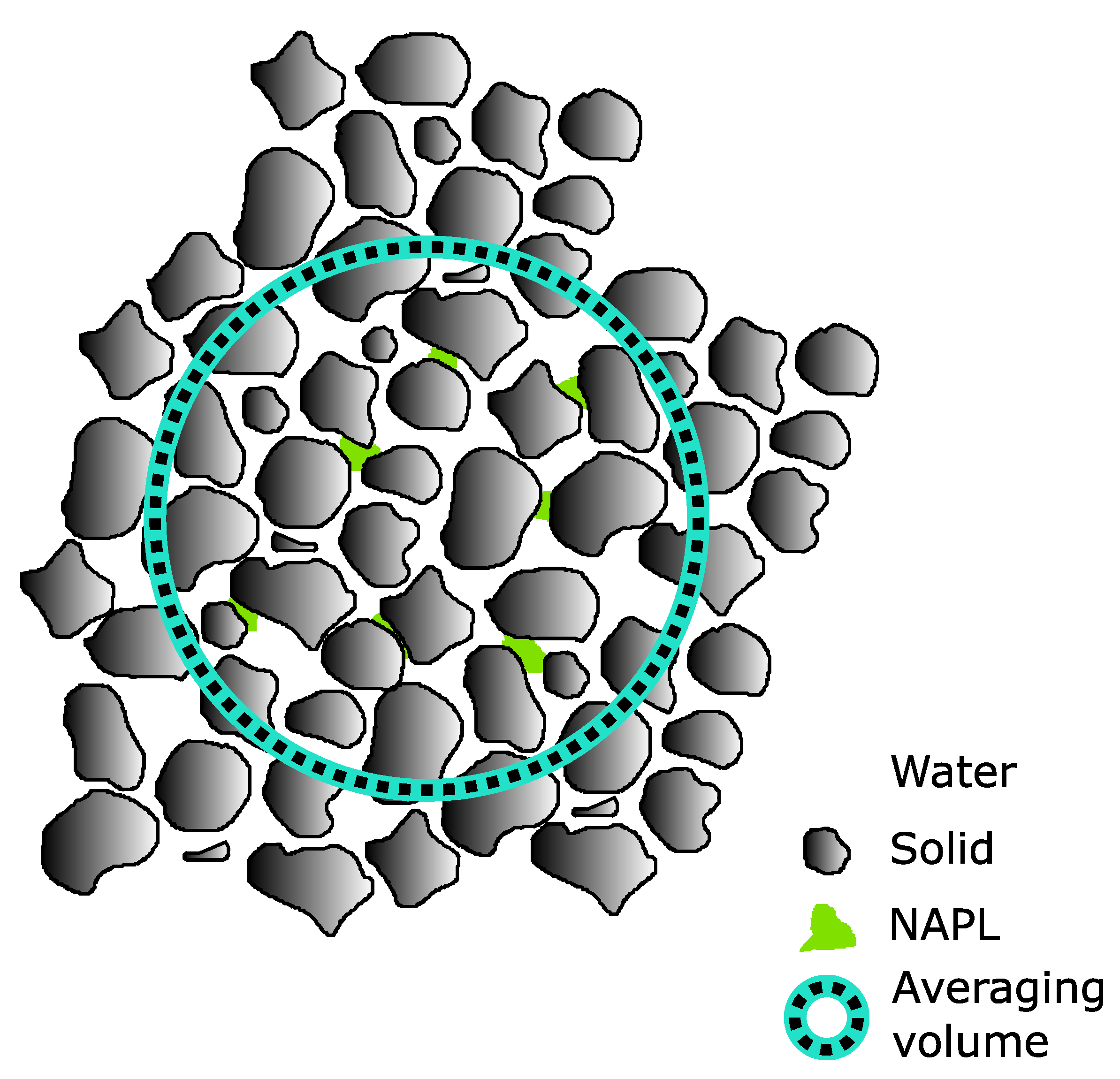
We are attempting to model a three-phase system, a characteristic portion of which is illustrated in Figure 1, each phase of which occupies a respective volume fraction of averaging domain , , and , which satisfy
We assume that the Darcy flux, , for the system as a whole is fixed and satisfies . Then, it follows from the chain rule and the fact that , that
The ADE applies in the water phase:
The solid and NAPL phases are homogeneous and do not need internal mass balance equations. However, the NAPL phase shrinks over time, yielding space to the water phase. This mass balance can be expressed by:
We work extensively with this term and so make the definition
where Q represents the upscaled source per unit time from the NAPL phase into the water phase.
2.2. Coupling Conditions
We assume no-slip boundary conditions, local equilibrium at the surface of the NAPL and no flux into the solid. Mathematically, these boundary conditions are expressed:
The solid volume fraction does not change with time, so the volume fractions can be coupled according to the following relationship:
3. Simplified Volume Averaging Analysis
We begin by applying the superficial averaging operator to (10), yielding
We manipulate each of the three terms separately to write them all in terms of intrinsic volume averages, simplifying each. We then assemble them and simplify further.
3.1. Accumulation Term
There is next to no analysis required here. The accumulation term can be expressed in terms of intrinsic volume averages directly
3.2. Advection Term
From volume averaging theorem (5):
from which it follows from no-slip conditions (13) and (14), that . Further simplification follows from writing c and in terms of their volume average and a perturbation: , and . Then, we may write . We have
Note that we can manipulate this by applying (9), so that
which can be back-substituted into (21), canceling and leading to the conclusion
For our purposes, we are primarily interested in the form of the source terms. It may thus be reasonable to employ a mean field approximation and discard the small double fluctuation term , however we retain it presently, later to be incorporated into an effective dispersion.
3.3. Diffusion Term
Again applying volume averaging theorem (5), we see that
or, by application of the no-flux boundary conditions, that
where we observe by direct inspection that the second term is a volumetric NAPL sink, representing diffusion of solute from the water phase into the NAPL. We thus replace it with the symbol , as defined in (12), emphasizing this role. By another application of an averaging theorem (4), it follows that
We now strongly diverge from the approach in Reference [13]. We eliminate the middle term on the RHS by noting that the average of at the elements of intersecting any plane is , and that V can be partitioned into planar slices, each orthogonal to , on which the expected value of c is constant. Assuming ergodicity, we conclude that the portion in square brackets is , independent of location, meaning that its divergence is also zero. To simplify the third term, we apply a result developed in Appendix B (). Observing that everywhere on , we see that:
Thus,
3.4. Assembly and Simplification of Governing Equation
Inserting (19), (23), and (28) into (18), and placing the variables in each of the terms in a consistent order yields:
We here diverge again from the customary volume averaging approach by immediately making the closure approximation . Customarily, this relationship would emerge from solution of a closure problem, as in Reference [9]. However, this particular dispersive flux relationship is “common practice” [23] (p. 174) textbook material (see also Reference [24], p. 244) and does not affect the form of the NAPL source term, which is the focus of the analysis in this note. Thus, we take the liberty of skipping its derivation.
This can be rearranged with its LHS containing only standard transport terms, and its RHS “source” terms relating to the dissolution of the NAPL:
We simplify this equation by noting that , and since the water phase solute concentration is dilute, . It follows immediately that :
The LHS of this equation resembles the desired advection-dispersion equation (multiplied through by ). A necessary condition for this to reduce to an ADRE with Sherwood-Gilland source (which depends on only the concentration difference ) to apply, the equation must simplify so that the mixed gradient term (proportional to ) on the RHS is eliminated. Doing so requires special assumptions. We consider one such case below.
3.5. Special Case: Advection Domination
In light of the failure to find an ADRE with Sherwood-Gilland source under general conditions, we follow Reference [17] in considering strongly advective conditions, which we here define as conditions in which . As is less than unity, has a system minimum value above zero, and is a volume averaged quantity, . Thus, under sufficiently strongly advective conditions, , allowing neglect of the term on the RHS of (32), as its coefficient is dominated by the one on the LHS. In such a case, one may simplify:
In order to close the system, we need a second equation to relate and . Note also that we are aiming to upscale the dissolution dynamics, and we only have a microscopic equation for Q, which is expressed in terms of the local concentration c, rather than the needed, upscaled . To solve both problems, we require an ansatz relating Q to and , for which we consider the Sherwood-Gilland relation. We stress, lest there be any confusion that we “get out what we put in,” we are not deriving the Sherwood-Gilland formulation from first principles in this section, only considering whether it is consistent with the microscopic formulation presented in Section 2. In the context of our analysis, this means that substitution into (33) ought to transform it to be similar to (7). For our analysis, we combine certain quantities defining the mass-transfer coefficient K in (2) into a single parameter, , and write
From dimensional considerations, it is clear that has units of and we observe that it plays the role in the above equation of the squared reciprocal of a characteristic length (“boundary layer”) for Fickian diffusion. Substituting (12), the definition for Q, into (34) yields:
This is a second, independent equation in terms of our dependent variables and . To arrive at (7), it then suffices to establish that . For , a characteristic value in the middle of the range of proposed values of (recall that these ranged from 0.6 to 1.24), (35) can be solved explicitly using the usual strategy for first-order non-homogeneous equations to generate
By differentiating (36), we observe that
Recalling that L is the length scale of the averaging volume, we see that
where the last inequality follows because the length scale of pore scale diffusion is small relative to the length scale of volume averaging. Because NAPL are sparingly soluble, it follows that . We may understand as an expected number of boundary layer length scales traversed by a solute particle due to diffusion since source emplacement. As long as , it follows that and thus that
Under these specific conditions, to the extent that can be treated as approximately constant (for instance, if everywhere ), we do recover the ADRE with Sherwood-Gilland source term.
4. Conclusions
In this note, we consider the dissolution of residual NAPL in saturated porous media by means of a nonstandard volume averaging analysis. Our approach applies a variety of strategies (including direct application of boundary conditions, a physics-preserving domain simplification, elimination of coefficient-dominated terms, a geometric lemma, and some other physically-grounded approximations) to simplify the phase boundary jump discontinuity terms that arise under superficial volume averaging and perform analysis using only the volume averaged equation. This is in contrast with the traditional volume averaging approach which entails developing a separate equation for concentration fluctuations which contains volume averaged terms such as “sources,” and formally closing the system by solving one or more boundary value problems to determine the functional form of the dependence of the fluctuations on the volume averaged quantities and then substituting these back into the volume averaged equation. The analysis here is radically simplified.
The particular problem we consider is whether Sherwood-Gilland empirical models are consistent with the micro-scale physics. Existing volume averaging analyses have led to equations that look much unlike the ADRE with a Sherwood-Gilland-type source, so this was a topic worth considering explicitly. The only attempt to recover a Sherwood-Gilland formula that we are aware of in the previous literature is due to Reference [17]: the form is recovered by applying four separate scale constraints that are defined in terms of the formal solutions to fluctuation boundary value problems formulated as part of the volume averaging process. Unfortunately, it is difficult to predict a priori whether these constraints are satisfied. Above, we derive the volume-averaged transport equation using the simplified volume averaging approach and find it is not an ADRE with a Sherwood-Gilland source term. We subsequently consider a physical restriction of advection-dominated behavior, but unlike Reference [17], it only requires a single restriction on the strength of advective transport relative to dispersive transport. We explicitly corroborate usage of the Sherwood-Gilland source model with the ADRE under such conditions when .
Funding
This research received no external funding; SKH holds the Helen Unger Career Development Chair in Desert Hydrogeology.
Conflicts of Interest
The author declares no conflict of interest.
Appendix A. Nomenclature
Here, we summarize the algebraic symbols and special operators introduced in this note. Phase subscripts or superscripts i and j are placeholders for any of the three phases in the system: n for NAPL, s for solid, and w for water. Bold is used to denote vector and matrix quantities (with the indicated dimensions applying to each component), with ordinary-weight Roman text denoting scalars. Dimensions are encoded in accordance with the SI standard: M for mass, L for length, and T for time, with a one indicating a dimensionless quantity.
| Symbol | Dimensions | Description |
| Superficial volume average operator | ||
| Intrinsic volume average operator for i phase | ||
| Locus of interface between phases i and j within V | ||
| Spatial region with centroid at over which volume averaging occurs | ||
| Fitted constant in empirical model of mass transfer coefficient K | ||
| Fitted exponent in empirical model of mass transfer coefficient K | ||
| Fitted exponent in empirical model of mass transfer coefficient K | ||
| Fraction of V occupied by i phase | ||
| Mass transfer coefficient in (6), as derived in [13] | ||
| Density of NAPL | ||
| Mass transfer coefficient | ||
| c | Chemical concentration in the water phase | |
| Thermodynamic saturation chemical concentration in the water phase | ||
| Characteristic length of porous media | ||
| Velocity-like closure variable in (6), as derived in [13] | ||
| Effective Fickian dispersion coefficient | ||
| Dispersion-like closure variable in (6), as derived in [13] | ||
| Infinitesimal surface element on | ||
| Infinitesimal volume element | ||
| Fickian diffusion constant | ||
| Indicator function for location belonging to the i phase | ||
| k | Closure variable representing dispersive flux | |
| K | Mass transfer coefficient from NAPL to water phase | |
| L | Length scale of averaging volume; | |
| Normal vector on interface directed from i phase into j phase | ||
| Darcy velocity near NAPL source zone | ||
| Q | Strength of NAPL-to-water mass source | |
| Re | Reynolds number | |
| NAPL saturation () | ||
| t | Time | |
| Velocity-like term in (6), as derived in [13] | ||
| Pore water velocity | ||
| Physical volume of V | ||
| Spatial position vector |
Appendix B. Derivation of a Geometric Lemma
This is a simplification of a “geometric lemma” presented by Whitaker on p. 17 of [9]. The derivation follows from use of a conceptual simplification of the domain—eliminating all NAPL-solid interfaces by imagining an infinitesimally thin water layer between the NAPL and the solid—that we show does not alter the flow or transport in the system or the volume averaging mathematics. Physically, because of the no-slip boundary conditions, there is no flow in the new notional, infinitesimally-thin water layers. Because any solute in these layers is at , no net NAPL-water mass transfer takes place there. And because the “new” water has infinitesimal volume, it represents a negligible source of mass into the existing pore water phase at the former NAPL-water-solid three-way interfaces. Mathematically, this simplification eliminates the interface , therefore eliminating terms of the form , for arbitrary f, when the appropriate volume averaging theorem is applied. Instead, new (collocated) interfaces and come into being. However, for any f, because and are the same surface, and the two integrals have opposite-directed normal vectors. Thus, the mathematics of volume averaging are unchanged.
Having established that we are always justified in assuming no NAPL-solid interface, the geometric lemma follows from application of volume averaging theorem (4) to an indicator function, , representing the presence of the water phase:
noticing that everywhere (except for jump discontinuities) is a constant, so and . Thus,
We may apply identical analysis to the solid phase:
but notice that because porosity is constant, . Furthermore, because we have notionally eliminated the NAPL-solid interface by imagining an infinitesimal layer of saturated, immobile water phase between them,
Noting that , it follows immediately from (A2) that
References
- Miller, C.; Poirer-McNeill, M.; Mayer, A.S. Dissolution of Trapped Nonaqueous Phase Liquids: Mass Transfer Characteristics. Water Resour. Res. 1990, 26, 2783–2796. [Google Scholar] [CrossRef]
- Imhoff, P.T.; Jaffe, P.R.; Pinder, G.F. An experimental study of complete dissolution of a nonaqueous phase liquid in saturated porous media. Water Resour. Res. 1993, 30, 307–320. [Google Scholar] [CrossRef]
- Powers, S.E.; Abriola, L.M.; Weber, W.J. An experimental investigation of nonaqueous phase liquid dissolution in saturated subsurface systems: Transient mass transfer rates. Water Resour. Res. 1994, 30, 321–332. [Google Scholar] [CrossRef]
- Saba, T.; Illangasekare, T.H. Effect of groundwater flow dimensionality on mass transfer from entrapped nonaqueous phase liquid contaminants. Water Resour. Res. 2000, 36, 971–979. [Google Scholar] [CrossRef]
- Nambi, I.M.; Powers, S.E. Mass transfer correlations for nonaqueous phase liquid dissolution from regions with high initial saturations. Water Resour. Res. 2003, 39. [Google Scholar] [CrossRef]
- Hossain, S.Z.; Mumford, K.G.; Rutter, A. Laboratory study of mass transfer from diluted bitumen trapped in gravel. Environ. Sci. Process. Impacts 2017, 19, 1583–1593. [Google Scholar] [CrossRef]
- Sherwood, T.K.; Gilliland, E.R. Diffusion of Vapors through Gas Films. Ind. Eng. Chem. 1934, 26, 1093–1096. [Google Scholar] [CrossRef]
- Kokkinaki, A.; O’Carroll, D.M.; Werth, C.J.; Sleep, B.E. An evaluation of Sherwood-Gilland models for NAPL dissolution and their relationship to soil properties. J. Contam. Hydrol. 2013, 155, 87–98. [Google Scholar] [CrossRef]
- Whitaker, S. The Method of Volume Averaging; Springer: Berlin/Heidelberg, Germany, 1999; p. 221. [Google Scholar]
- Whitaker, S. Diffusion and Dispersion in Porous Media. AIChE J. 1967, 13, 420–427. [Google Scholar] [CrossRef]
- Slattery, J.C. Flow of Viscoelastic Fluids Through Porous Media. AIChE J. 1967, 13, 1066–1071. [Google Scholar] [CrossRef]
- Wood, B.D. The role of scaling laws in upscaling. Adv. Water Resour. 2009, 32, 723–736. [Google Scholar] [CrossRef]
- Quintard, M.; Whitaker, S. Convection, dispersion, and interfacial transport of contaminants: Homogeneous porous media. Adv. Water Resour. 1994, 17, 221–239. [Google Scholar] [CrossRef]
- Porta, G.M.; Riva, M.; Guadagnini, A. Upscaling solute transport in porous media in the presence of an irreversible bimolecular reaction. Adv. Water Resour. 2012, 35, 151–162. [Google Scholar] [CrossRef]
- Porta, G.M.; Ceriotti, G.; Thovert, J.F. Comparative assessment of continuum-scale models of bimolecular reactive transport in porous media under pre-asymptotic conditions. J. Contam. Hydrol. 2016, 185–186, 1–13. [Google Scholar] [CrossRef]
- Ma, Y.; Mohebbi, R.; Rashidi, M.M.; Manca, O.; Yang, Z. Numerical investigation of MHD effects on nanofluid heat transfer in a baffled U-shaped enclosure using lattice Boltzmann method. J. Therm. Anal. Calorim. 2019, 135, 3197–3213. [Google Scholar] [CrossRef]
- Quintard, M.; Whitaker, S. Dissolution of an Immobile Phase during Flow in Porous Media. Ind. Eng. Chem. Res. 1999, 38, 833–844. [Google Scholar] [CrossRef]
- Bahar, T.; Golfier, F.; Oltéan, C.; Benioug, M. An Upscaled Model for Bio-Enhanced NAPL Dissolution in Porous Media. Transp. Porous Media 2016, 113, 653–693. [Google Scholar] [CrossRef]
- Bahar, T.; Golfier, F.; Oltéan, C.; Lefevre, E.; Lorgeoux, C. Comparison of theory and experiment for NAPL dissolution in porous media. J. Contam. Hydrol. 2018, 211, 49–64. [Google Scholar] [CrossRef] [Green Version]
- Kechagia, P.E.; Tsimpanogiannis, I.N.; Yortsos, Y.C.; Lichtner, P.C. On the upscaling of reaction-transport processes in porous media with fast or finite kinetics. Chem. Eng. Sci. 2002, 57, 2565–2577. [Google Scholar] [CrossRef]
- Golfier, F.; Wood, B.D.; Orgogozo, L.; Quintard, M.; Buès, M. Biofilms in porous media: Development of macroscopic transport equations via volume averaging with closure for local mass equilibrium conditions. Adv. Water Resour. 2009, 32, 463–485. [Google Scholar] [CrossRef]
- Orgogozo, L.; Golfier, F.; Buès, M.; Quintard, M. Upscaling of transport processes in porous media with biofilms in non-equilibrium conditions. Adv. Water Resour. 2010, 33, 585–600. [Google Scholar] [CrossRef] [Green Version]
- Rubin, Y. Applied Stochastic Hydrogeology; Oxford University Press: New York, NY, USA, 2003; p. 391. [Google Scholar]
- Gelhar, L.W. Stochastic Subsurface Hydrology; Prentice-Hall: Englewood Cliffs, NJ, USA, 1993; p. 390. [Google Scholar]
Figure 1.
Schematic diagram of blobs of residual NAPL in pores defined by solid media otherwise saturated with water, with averaging volume superimposed.
Figure 1.
Schematic diagram of blobs of residual NAPL in pores defined by solid media otherwise saturated with water, with averaging volume superimposed.

© 2019 by the author. Licensee MDPI, Basel, Switzerland. This article is an open access article distributed under the terms and conditions of the Creative Commons Attribution (CC BY) license (http://creativecommons.org/licenses/by/4.0/).
Share and Cite
MDPI and ACS Style
Hansen, S.K. Exploring Compatibility of Sherwood-Gilland NAPL Dissolution Models with Micro-Scale Physics Using an Alternative Volume Averaging Approach. Water 2019, 11, 1525. https://doi.org/10.3390/w11071525
AMA Style
Hansen SK. Exploring Compatibility of Sherwood-Gilland NAPL Dissolution Models with Micro-Scale Physics Using an Alternative Volume Averaging Approach. Water. 2019; 11(7):1525. https://doi.org/10.3390/w11071525
Chicago/Turabian StyleHansen, Scott K. 2019. "Exploring Compatibility of Sherwood-Gilland NAPL Dissolution Models with Micro-Scale Physics Using an Alternative Volume Averaging Approach" Water 11, no. 7: 1525. https://doi.org/10.3390/w11071525
Note that from the first issue of 2016, this journal uses article numbers instead of page numbers. See further details here.