Fine Sediment Modeling During Storm-Based Events in the River Bandon, Ireland


1
Department of Mining and Civil Engineering, Universidad Politécnica de Cartagena, Paseo Alfonso XIII, 52, Cartagena 30203, Spain
2
School of Building & Civil Engineering and Sustainable Infrastructure Research & Innovation Group, Cork Institute of Technology, Rossa Avenue, Bishopstown, Cork T12 P928, Ireland
*
Author to whom correspondence should be addressed.
Water 2019, 11(7), 1523; https://doi.org/10.3390/w11071523
Submission received: 10 June 2019
/
Revised: 19 July 2019
/
Accepted: 19 July 2019
/
Published: 23 July 2019
(This article belongs to the Section Hydraulics and Hydrodynamics)
Abstract
:The River Bandon located in County Cork (Ireland) has been time-continuously monitored by turbidity probes, as well as automatic and manual suspended sediment sampling. The current work evaluates three different models used to estimate the fine sediment concentration during storm-based events over a period of one year. The modeled suspended sediment concentration is compared with that measured at an event scale. Uncertainty indices are calculated and compared with those presented in the bibliography. An empirically-based model was used as a reference, as this model has been previously applied to evaluate sediment behavior over the same time period in the River Bandon. Three other models have been applied to the gathered data. First is an empirically-based storm events model, based on an exponential function for calculation of the sediment output from the bed. A statistically-based approach first developed for sewers was also evaluated. The third model evaluated was a shear stress erosion-based model based on one parameter. The importance of considering the fine sediment volume stored in the bed and its consolidation to predict the suspended sediment concentration during storm events is clearly evident. Taking into account dry weather periods and the bed erosion in previous events, knowledge on the eroded volume for each storm event is necessary to adjust the parameters for each model.
1. Introduction
Compliance with the European Union Water Framework Directive, the Freshwater Fish Directive, and the Habitats Directive requires the monitoring and modeling of fine sediment behavior and concentrations in riverine systems. Modeling provides an understanding of the dynamics of suspended sediment flux and allows the study of impacts of fine sediments on, for example, riverine fish populations [1,2,3,4,5,6]. Different types of model are commonly used to quantify the suspended sediment concentration, SSC, in gravel-bed rivers. These can be based on the classical equation SSC = aQb, which directly relates flowrate (Q) with suspended sediment concentration, with the use of constants a and b being empirically adjusted, as is presented in Harrington and Harrington [7,8]. Other models are empirically-based, such as that of Park and Hunt [1], to quantify the fine sediment volume stored and eroded on a continuous time basis in the stream bed, i.e., during storm events and during dry weather periods. In their model, the storage and erosion of the sediment bed reservoir are based on exponential functions. Vansickle and Beschta [2] proposed an empirically-based model for storm events that takes into account sediments stored in the bed and also allows calculation of the SSC in the streamflow during storm events. Other models are statistically-based [3,4] and were originally proposed to predict the pollutograph, i.e., the concentration of a substance transported in a sewer like-flow during storm events. This is achieved by predicting three points of the SSC–time curve: the maximum concentration, Cmax; the time to the peak concentration, TPE; and the time from descent from the peak concentration, TDE. From these three points, exponential and logarithmic curves are proposed to represent the complete curve. Other classical models [9,10] are based on shear stress values in the bed, proportional to the bed erosion transported due to the streamflow. These models based on shear stress use an erosion rate, M, with erosion commencing when a critical value of shear stress, τc, is exceeded. Other authors have previously studied storm events to quantify the fine sediment transport within a reach in a gravel bed river [11,12] through field measurements, considering important aspects such as sediment storage in the mainstream channel and its evolution during inter-event periods. The relationship between suspended sediment concentration, SSC, and fine sediment ingress into gravel bed rivers has been experimentally studied through sediment traps installed in the bed of the stream [13,14]. In general, factors that influence the suspended sediment load during storm events have been extensively studied in recent decades, although much effort is still needed to provide models with the capacity to predict the SSC with low uncertainty indices [5,6,7,8,15,16,17].
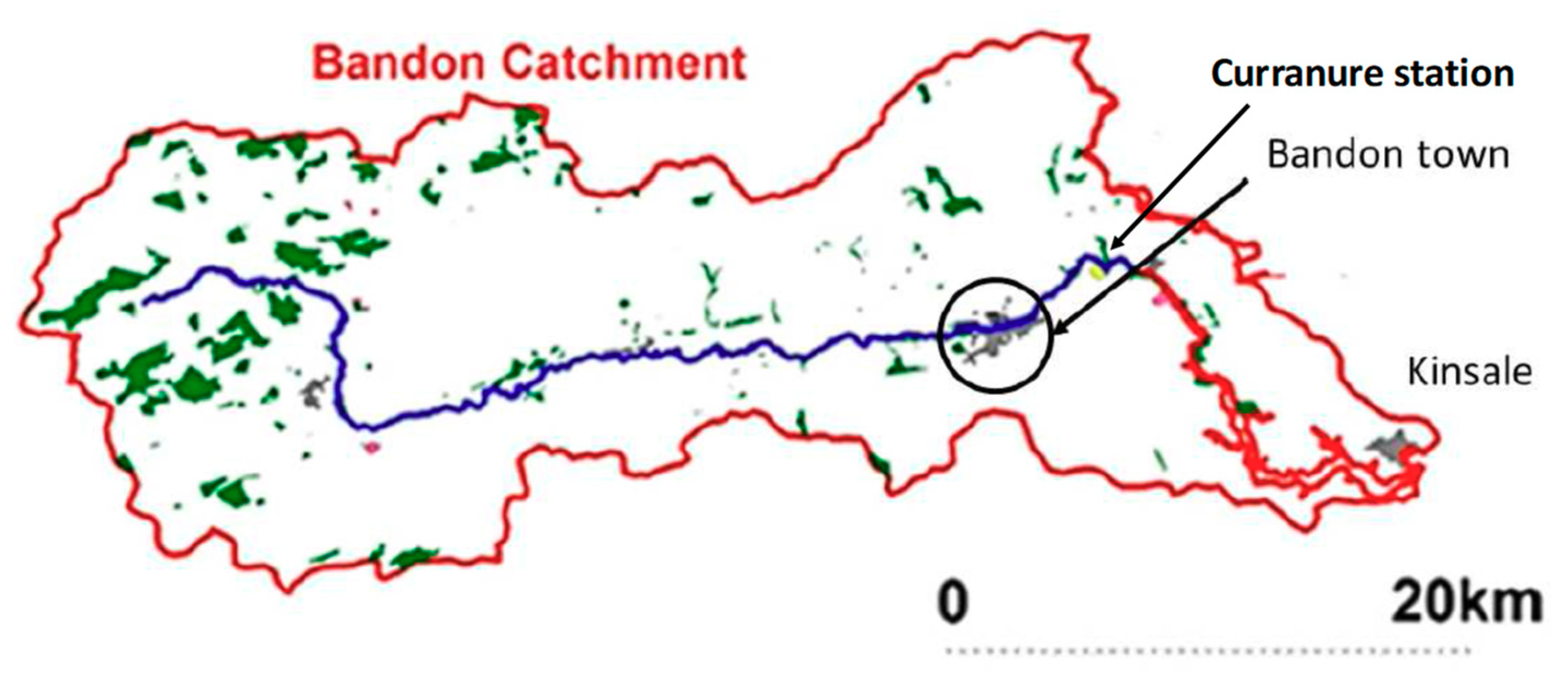
The work presented in this paper evaluates the SSC concentration in the River Bandon, Ireland, during the period from 10 February 2010 to 9 February 2011 at the Curranure gauging station (Figure 1). Three different models are proposed to calculate the SSC during 27 storm events over this period. One is the empirically-based model of Vansickle and Beschta [2], modified due to the introduction of a variable parameter to take into account the variation of the bed storage and its consolidation. The others are the statistically-based model of Garcia et al. [3,4] and a shear stress-based model. The total accumulated value of suspended sediments mobilized at each storm event is compared with measured values. The uncertainty involved is calculated and discussed. The importance of accounting for the storage of fine sediments in the bed and its consolidation in the different models is the most important aspect of the work presented.
2. Materials and Methods
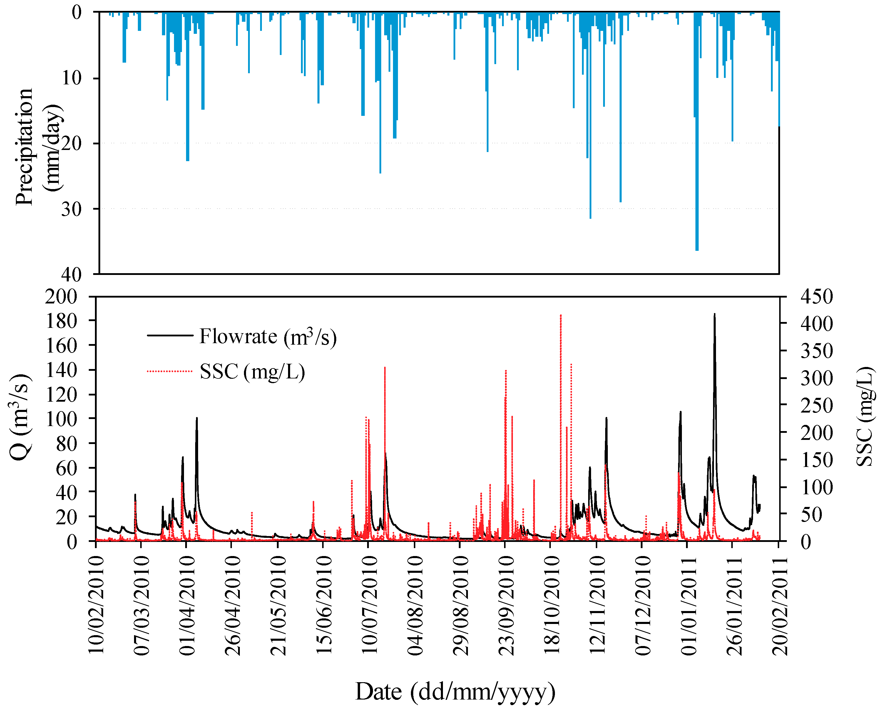
The River Bandon, County Cork (Ireland), has been time-continuously monitored by turbidity probes, as well as automatic and manual suspended sediment sampling, for a number of years. Figure 2 presents the Q and SSC values recorded over the period from 10 February 2010 to 9 February 2011 at the gauging station at Curranure. The daily total precipitation at the Cork Airport station is also included in this figure. The Office of Public Works (OPW) monitors the flow rate of the River Bandon and digitizes 15 min flow data, that are available from 1976 in the Curranure station, which is the same location where the Cork Institute of Technology (CIT) disposes the turbidimeter. These data were analyzed and included in previous published works [8,11]. The Curranure gauging station on the River Bandon (co-ordinates: 51.766, −8.682) has a catchment area of 424 km2 and drains approximately 70% of the entire River Bandon catchment. Fully digitized 15 min flow rate data are available from 1976 onwards. The turbidity probe takes a reading every 15 s. The data controller generates an output based on the average of a 15 min interval. This means each recorded data point is the average of 60 scans over 15 min. The turbidity data is calibrated with manual and automatic sampling [5,6,7,8]. In the case of model simulations, these are taken each 15 min, except for the bed shear stress model, for which, due to the numerical conditions (courant number < 0.5), the simulation period is 5 s.
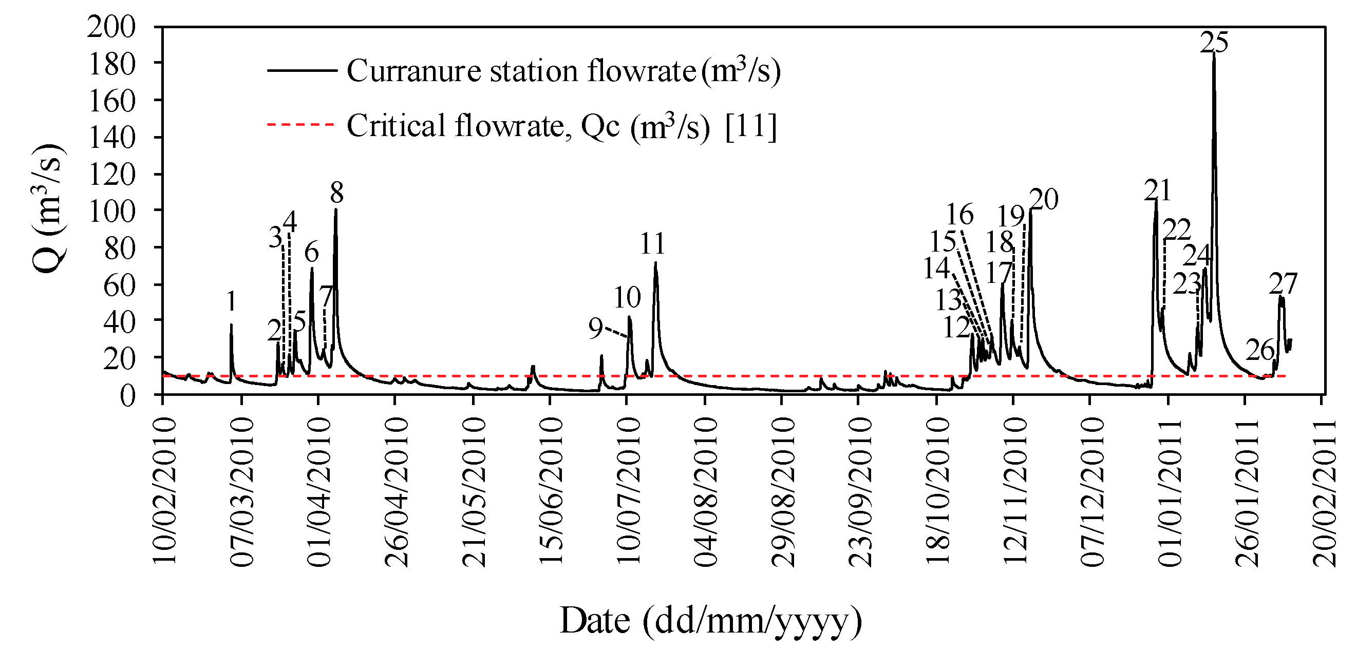
This data was evaluated by Park [11] using a slope–break analysis which proposed that for the River Bandon, the critical flowrate, Qc, should be adopted as 10 m3/s. Flow rates greater than this critical flow give rise to sediment bed erosion, transport, and fine sediment suspension. Visual observation and field experience [18] have shown that the bed load becomes active in the range of 10 to 15 m3/s, which is in agreement with the results of the slope–break analysis developed by Park [11]. The hydrograph separation between a storm event flow from base flow has been addressed by several authors like [19]. Methods can be graphical or tracer-based, among others. In the present work, as was stated in [1] and [11], the base flow is considered as a flowrate lower that the critical flow, Qc = 10 m3/s. Above this flowrate, it is considered as part of a storm event. The identification of independent storm events requires the start and end times of these events in the flowrate record to be determined. This is usually done manually by visual inspection of the time series data, as stated by [20]. Automatic event identification methods could be applied to large data records, although this requires manual supervision, as proposed by [21]. In the present work, once the critical flow is exceeded and a recession curve is observed, this is manually identified as an independent event. Figure 3 presents the storm-based events considered in the present work, where the critical flowrate (10 m3/sec) is reached and exceeded. These 27 storm events will be individually studied using each of the three formulations proposed and model values will be compared with measured results.
The models proposed are used only for the storm event periods, i.e., from once the critical flow is achieved until the flow decreases to approximately Qc again. The independent storm events were considered when the following conditions were achieved: (i) flowrate was greater than the critical flow, Qc, that is, when sediment bed erosion, transport, and fine sediment suspension were observed, as presented in Figure 3; (ii) a peak in the measured suspended sediment concentration was observed; and (iii) the total event suspended sediment during the episode, ESS, >0.5 (tons). This criterion was adopted with the intention of reproducing all the peaks of SSC and, from this, all the volumes eroded by storm events, and understood as those that occur under the above conditions.
Due to this, and to the fact that the fulfilment of the soil reservoir of fine sediments is time-dependent, the proposed models in the present work make use of the Park [1,11] formulation during the inter-event periods, i.e., when the flowrate is less than Qc. During these time periods, Equation (1) regulates the fulfilment of the soil reservoir with fine sediments. Equation (2) is a simplified equation for the fine sediment transport SSC in the flowrate. Both equations are included as proposed by Park [11].
Here, S(t) and S(t+1) are the volumes of fine sediment in the bed stream (tons); C(t) is the SSC concentration (mg/L); α is a constant; and Smax is the maximum volume of fine sediment in the bed stream, calibrated by Park [11], where in the case of the River Bandon, a value of 430 tons is adopted. At the beginning of the simulation period, the fine sediment volume in the bed stream is taken as the Smax value.
Regarding the aspects related to the genesis of the suspended sediment concentration, we have to distinguish the following steps: (i) during the dry weather periods, when the flowrate is below the critical flow rate (Q < Qc), fine sediments end up settling on the bed or are transported in suspension in low concentrations. This sedimentation helps contribute to the cohesion and consolidation of sediments in the bed of the stream. The fine sediments are sourced from both the bed and the banks of different parts of the gravel bed river. Over a period of time, the bed will be filled with fine sediments and once filled, will then give rise to a decrease of sediment storage in the bed; (ii) once flow rates are greater than the identified critical flow, it gives rise to sediment bed erosion and sediment transport that increases the fine sediment in suspension. Visual observation and field experience have shown that the bed load becomes active in the range of 10 to 15 m3/s, which is in agreement with the results of the slope break analysis developed by Park [11]. In this situation, it usually coincides with rainfall events where fine sediment comes from the watershed, the bed, and the banks of the stream. All the fine sediments are transported by the vertical diffusion process from the bed of the stream, i.e., although they are sourced from the banks, bed, or watershed, all finish up in the bed and from there, are moved in suspension through a diffusive process. When we talk about fine sediment transported in suspension during storm events in this research, we are referring to sediments where the d90 ≈ 0.6 mm.
2.1. Vansickle and Beschta (1983) Modified
This model is proposed to estimate the SSC during storm events. The model includes four empirical constants: r and p are related to how sediment storage is emptied and its volume, whilst a and b are the constants in equation SSC = aQb whose initial values are taken from Harrington and Harrington [8]. Equations (3) and (4) detail the original model proposed [2].
Here, S(t) represents the volume of solids stored in the bed (tons); Smax is the maximum volume that can be stored in the bed, and adjusted to 430 tons for the River Bandon [11]; C(t) is the SSC concentration (mg/L); and Δt is the time interval, which, in this case, is 15 min. Equations (3) and (4) will be solved for the 27 storm events presented in Figure 3.
In this work, the original model equations will be modified to take into account the availability of fine sediment in the bed. This availability depends on variables such as the volume stored in the bed and the consolidation of this sediment volume, which are considered through the variables of the dry weather period and the volume eroded during the previous event. This assumes that the value of the r parameter will not be a constant parameter, whereas in the original work of Vansickle and Beschta [2], a constant value was adopted for all the storm events modeled.
2.2. Garcia et al. (2017, 2018) Modified
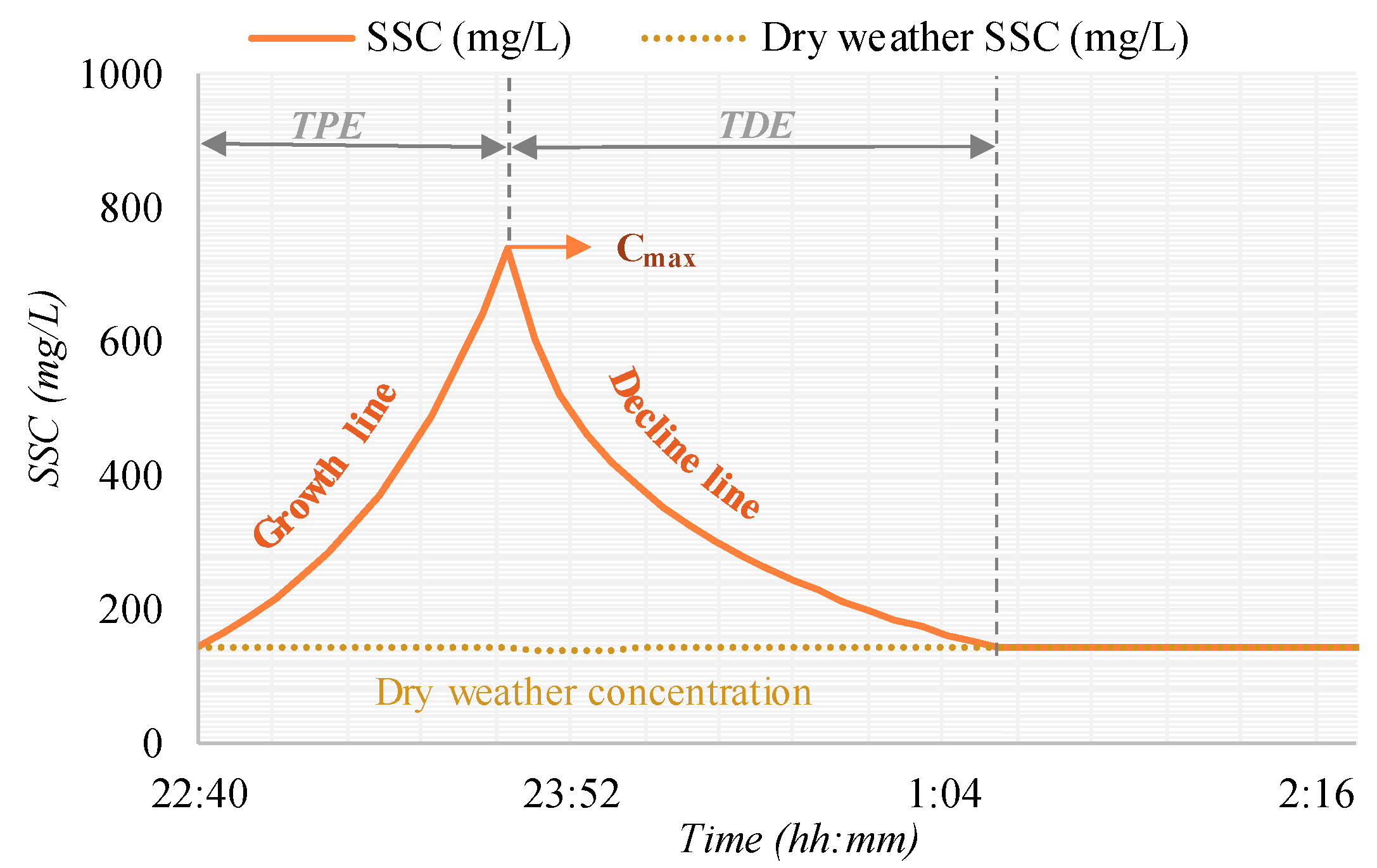
This formulation was originally developed for urban runoff during combined sewer overflows. The SSC curve during storm events is calculated from statistical indices. The first step is to calculate the following variables from the 27 storm events: the dry weather period between storm events, DWP (day); time to peak of the hydrograph measured from the time where the flowrate exceeds the critical flowrate proposed [11], TPH (day); time to peak of the SSC measured data, TPE (days), in each flooding event; maximum flowrate of each flood event, Qmax (m3/s); maximum SSC concentration measured in each event, Cmax (mg/L); time from the peak of the SSC curve to the end of the curve, TDE (day); and C0 dry weather concentration (mg/L). The next step is the adjustment of three linear regressions that relate the variables Cmax, TPE, and TDE with the hydraulic variables measured in the 27 available storm events: TPH, Qmax, and DWP. Once this is achieved, the SSC curve is constructed from these three points, as presented in Figure 4, using additional growth and decline curves.
2.3. Shear Stress Erosion-Based Formulation
A longitudinal advection and vertical diffusion suspended load approach with shear stress-related fine sediment erosion is presented. Equation (5) details the bed erosion process where the parameter M is expressed in mg/m2/hour. Precedents for shear stress erosion-based formulations can be found in [9,10].
Here, τb is the shear stress in the bed (Pa) calculated from the HEC-RAS calibrated model for the River Bandon, as presented in [22], and τc is the critical stress (Pa) based on the critical flowrate Qc [11]. The eroded or settled suspended sediment concentration, SSC, is presented in Equations (6) and (7) at the turbidity probe depth, Cl(t), according to [23], and due to the diffusion of eroded bed sediments.
In the case where τb < τc,
In the case where τb > τc,
where w is the fall velocity of a particle of 0.0625 mm (0.0012 m/s); Δt is the time interval of 5 s; Uc(t) is the shear velocity according to the HEC-RAS calibrated model in the River Bandon, as presented in [19]; k is the Von Karman constant; a_l is the height of the active layer considered as 0.04 m for this work, which corresponds with the depth of the active layer of the bed; h(t) is the flow depth [12]; and l is the height of the location of the turbidity probe that is calibrated from the manual and automatic sampling, which is 0.11 m above the bottom of the river.
Here, U represents the average horizontal component of the velocity in the stream, C is the suspended sediment concentration (mg/L), and E is the eroded or settled sediment balance at each time step. Equations (6), (7), and (8) are solved through a 1-D advection–erosion/settling–diffusion finite difference scheme forward in space and time, where the results are in agreement with a forward time centered space scheme [24,25], as presented in Equation (9), where the courant number is less than 0.5.
3. Results and Discussion
The values of the parameters adopted in each of the models evaluated will be described. The results of the SSC modeling are presented and compared with measured values. Finally, the uncertainty indices are calculated and compare the total budget of fine sediment eroded from the bed for each storm event. The total volume of fine sediment corresponding to each storm event, described as the event suspended sediment, ESS, is calculated considering the SSC of the rising limb (growth) section of each hydrograph minus the SSC that would correspond to the dry weather period, as stated in [1,11]. The SSC for the dry weather period was adjusted by the value SSC = 0.1Q for the River Bandon based on previous work [1]. Bank erosion is not treated separately in this work as it is considered a contributor to the bed storage, i.e., the bank erosion will contribute to the sediment bed of the stream and this bed sediment will then be mobilized and transported.
3.1. Vansickle and Beschta (1983) Modified
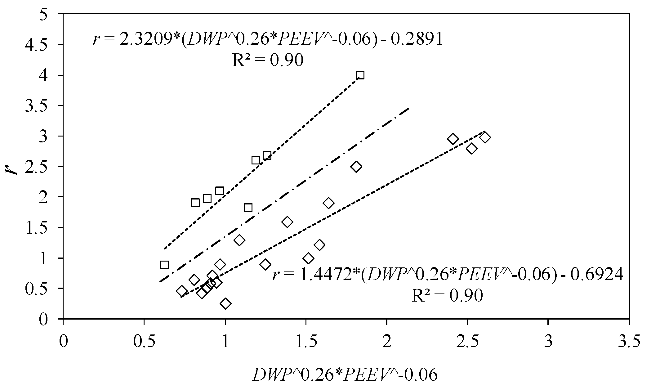
In this model, to adjust the measured SSC values and the fine sediments eroded from the bed, the r parameter of sediment availability in the bed storage is studied and proposed as a variable, which is different to the original model [2]. This r parameter was adopted as a variable with the intention of achieving the same eroded volume in each storm event as the measured volume. This gave rise to different values of the parameter r for each event. When representing this as a function of the dry weather period, DWP, and the previous event eroded volume, PEEV, it is observed that the value adopted by r shows two trends, that of Equation (10) in the case of high peaks of flow, or when a very low DWP is accompanied by a high value of PEEV for Equation (11):
Figure 5 shows the proposed adjustments employed to determine the r value.
The other parameters included in the model are presented in Table 1.
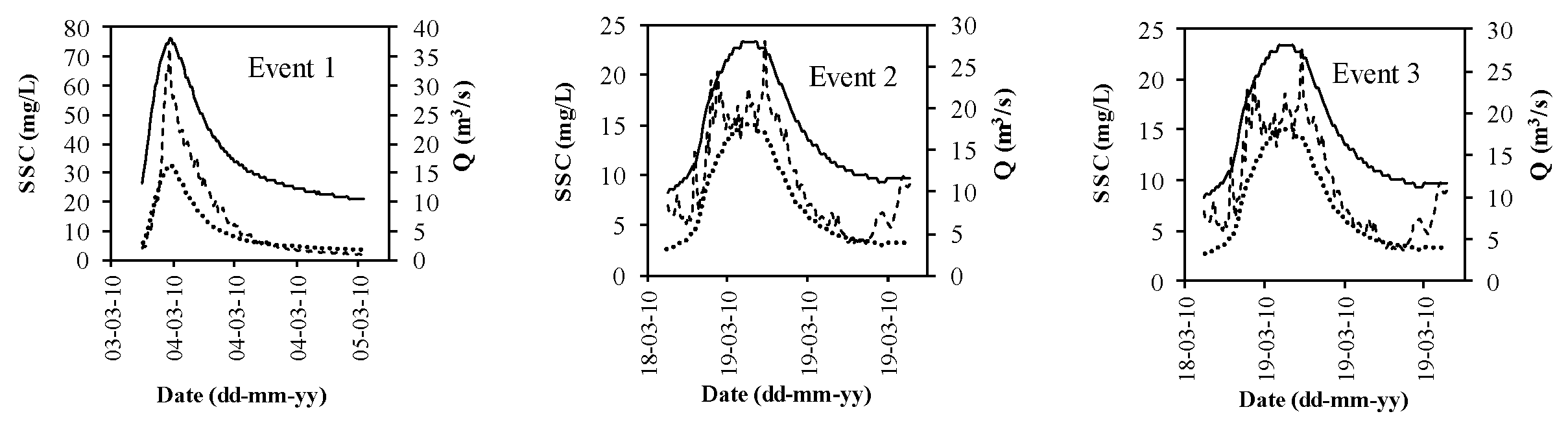
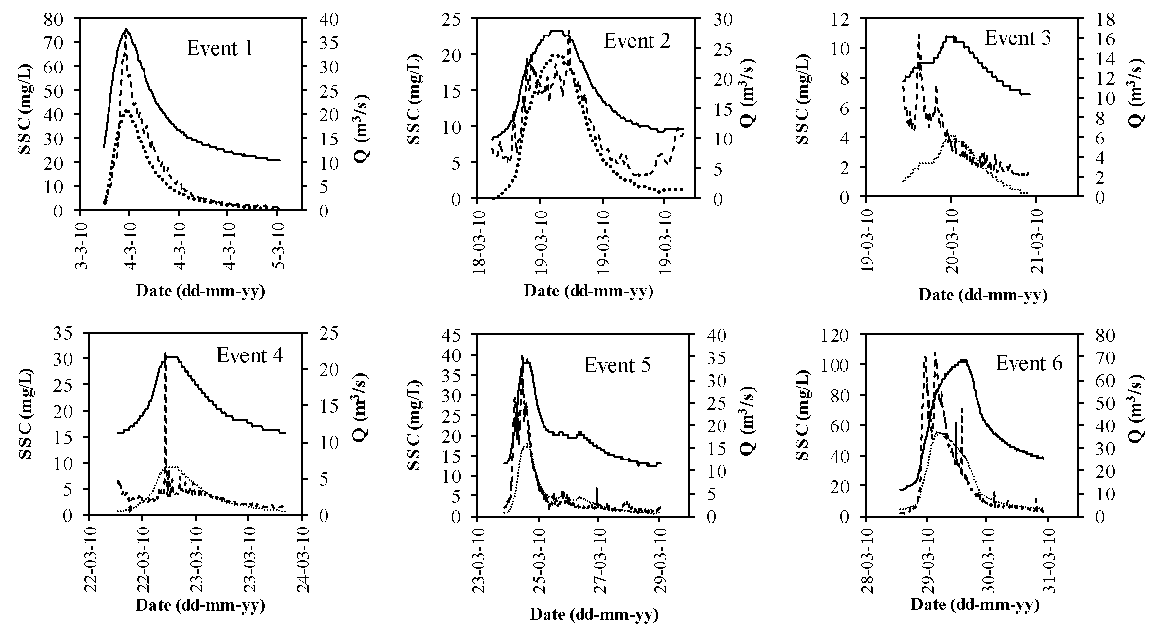
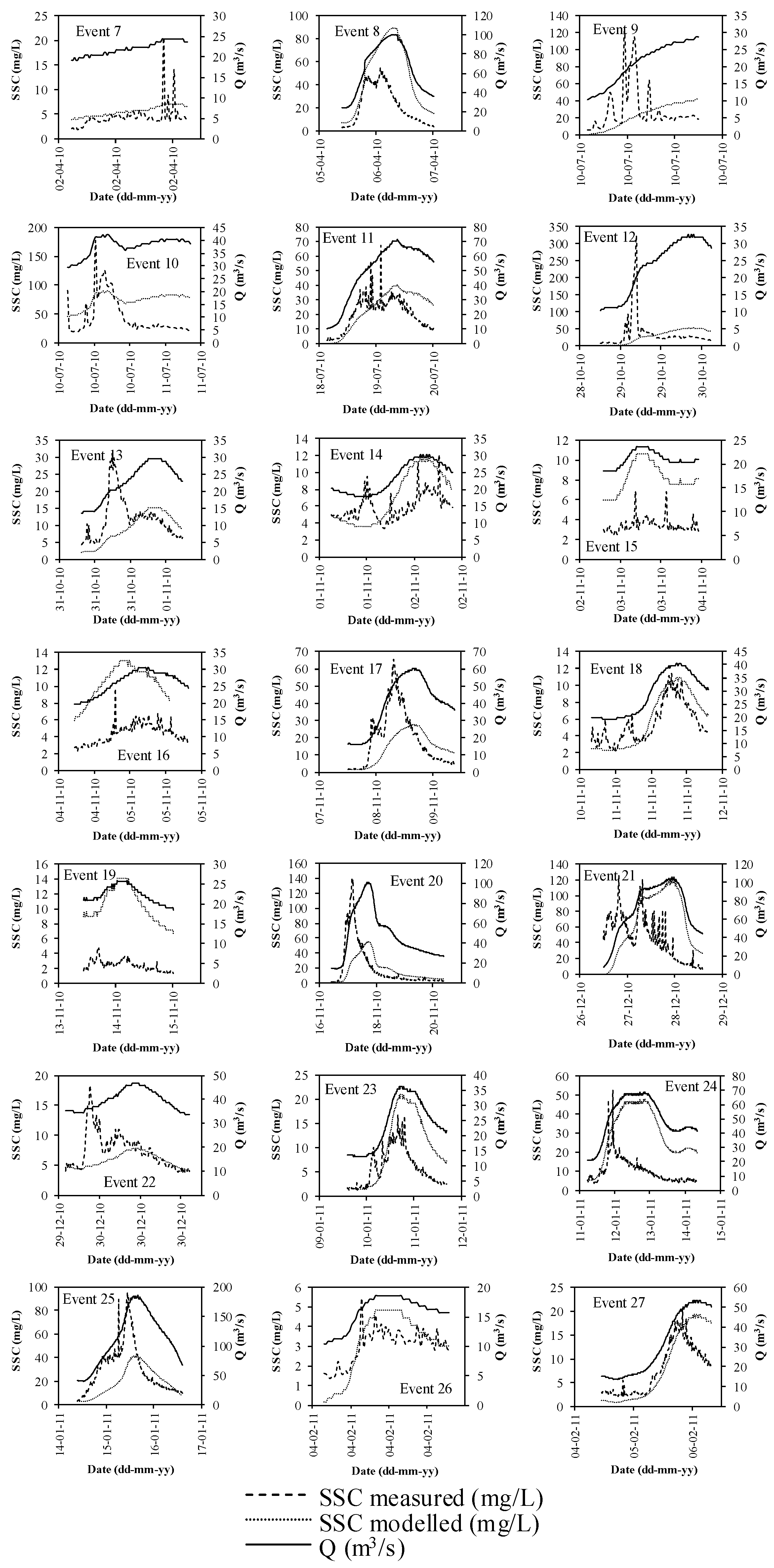
The variables a and b are in agreement with previous work undertaken on the River Bandon [8]. The r parameter is approximately in the 0.1 to 4 range. Figure 6 presents the 27 storm events considered, where the measured and calculated SSC values can be observed.
In general, the SSCs modeled with the Vansickle and Beschta [2] modified model present quite good agreement with the measured values. It can be observed that for almost all the modeled storm events, the trend of the SSC measured is predicted by the modeled data and some of the modeled event results correspond with the shape and with the SSC measured concentrations. Differences for some events presented through Figure 6 associated with high flows may be explained by an increase in bank erosion that finishes being transported as suspended sediment, as stated in [12]. Differences in erosion for similar events may be explained by differences in the consolidation of the fine sediment in the bed stream. To confirm these preliminary conclusions, it is recommended that field experimental campaigns of the fine sediments of the bed of the river be undertaken.
3.2. Garcia et al. (2017, 2018) Modified
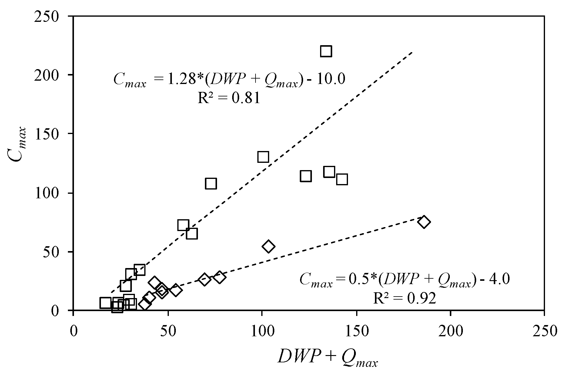
In this model, three linear regressions are presented in Figure 7 and Figure 8 that relate the variables Cmax, TPE, and TDE to the hydraulic variables measured in the 27 available storm events: TPH, Qmax, and DWP. The adjustment in the case of Cmax is presented in Equations (12) and (13) and in Figure 7. Two different trends are observed, representing the different behavior of fine sediment erosion in the studied events, where Equation (13) is related to higher peaks of flow and DWP. Further studies are needed for a better understanding of both trends that could be related to the availability and consolidation of fine sediment coming from the bed and the bank through the year:
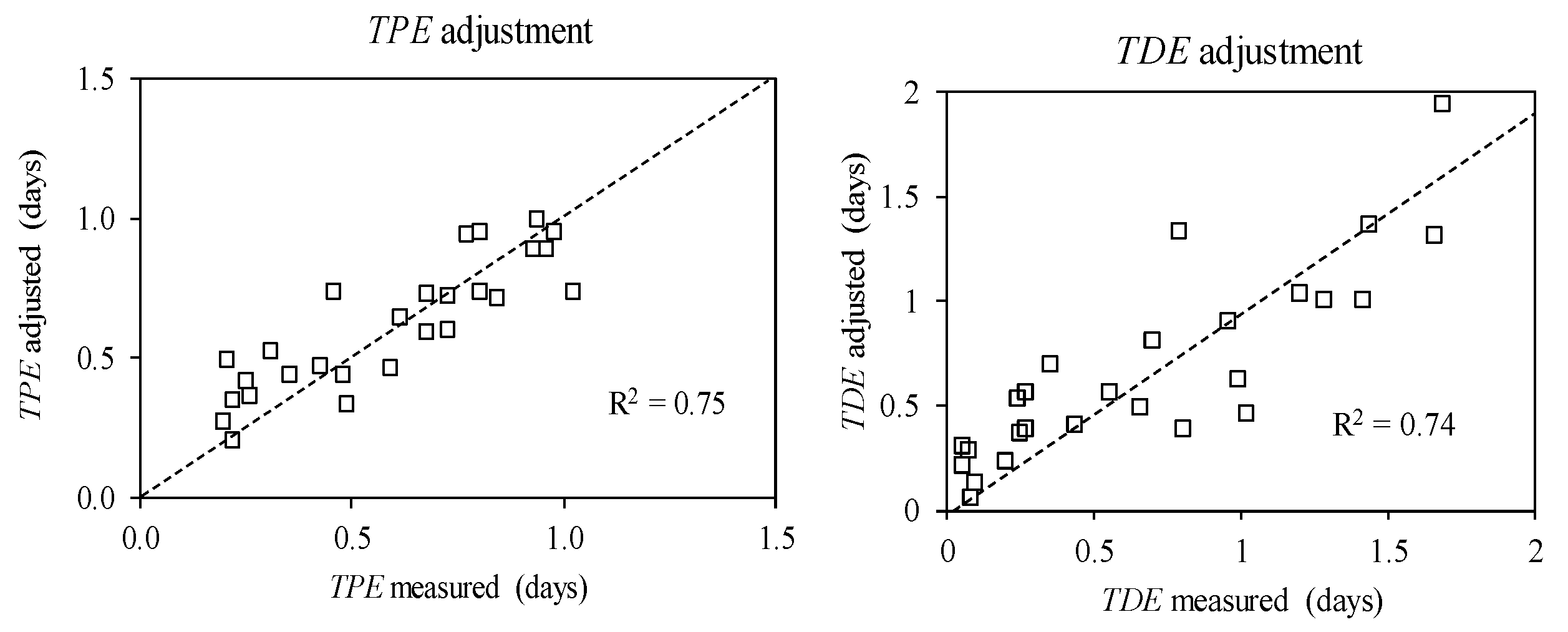
Equations (14) and (15) present the adjustments for the variables TPE and TDE, respectively. These are two linear regressions which compare hydraulic parameters such as the TPH, DWP, and Qmax. Figure 8 presents the goodness of the adjustment for both parameters.
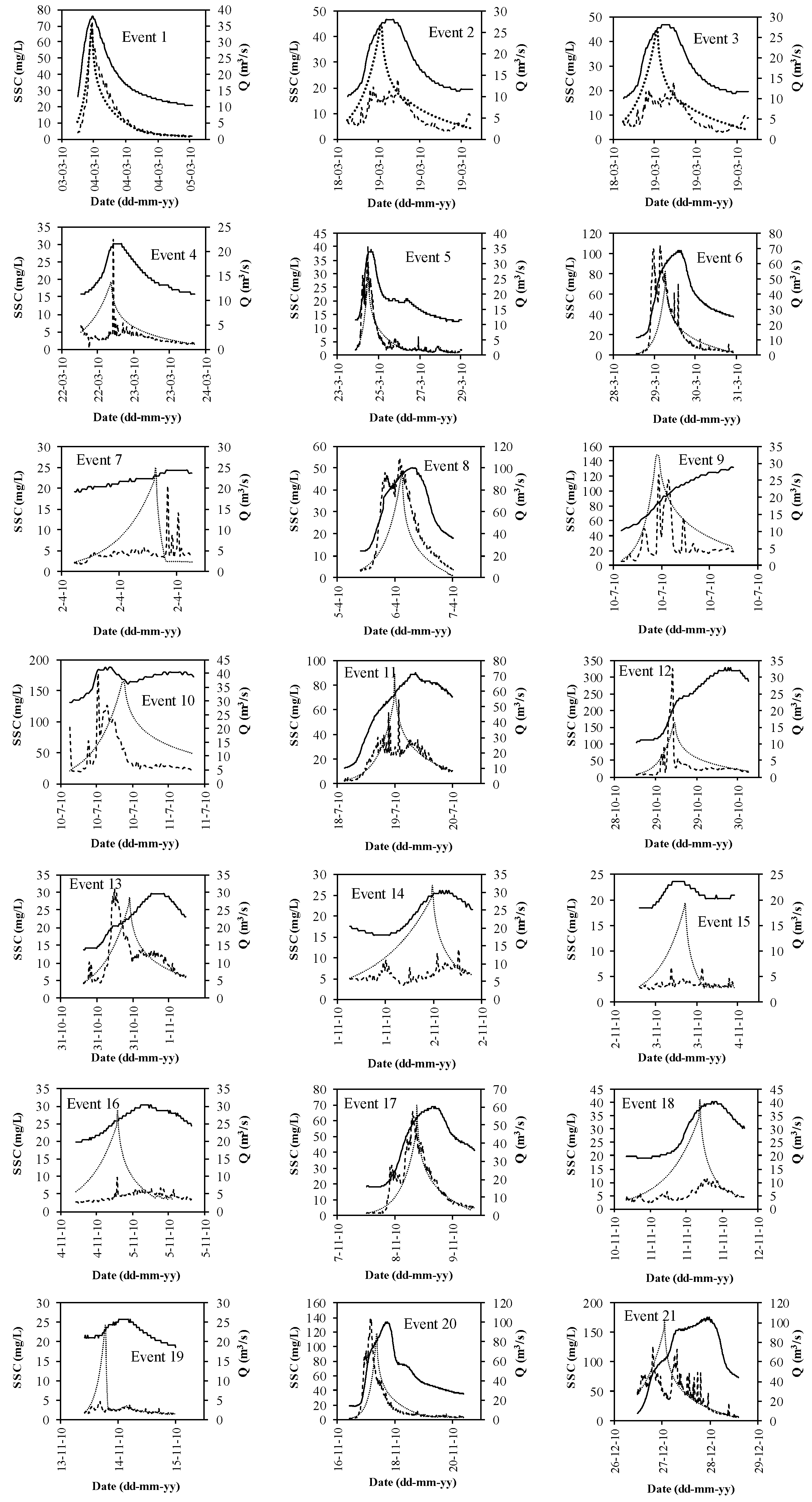
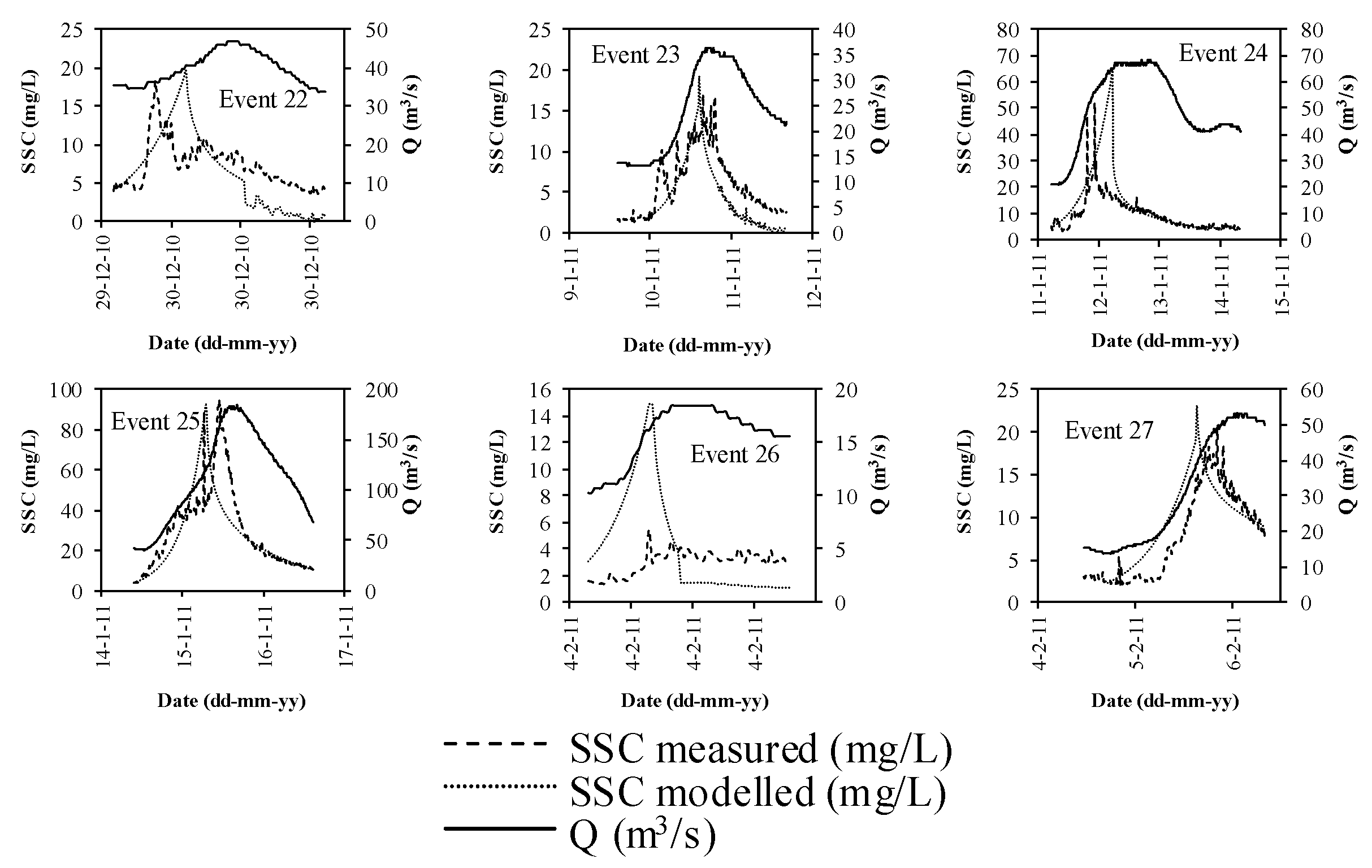
Figure 9 presents the 27 storm events considered, where the measured and calculated SSC values can be observed. In these figures, it can be observed that there is good agreement with the SSC measured for some events, such as event numbers 1, 5, 11, 17, 19, 23, 25, and 27. For other events, the SSC peak modeled overestimates the values measured in the field, such as for event numbers 2 and 3, and this indicates that the statistical model needs to be adjusted with additional storm events. In any case, the differences are acceptable and this formulation should be studied in greater detail with more field data and for new storm events.
3.3. Shear Stress Erosion-Based Formulation
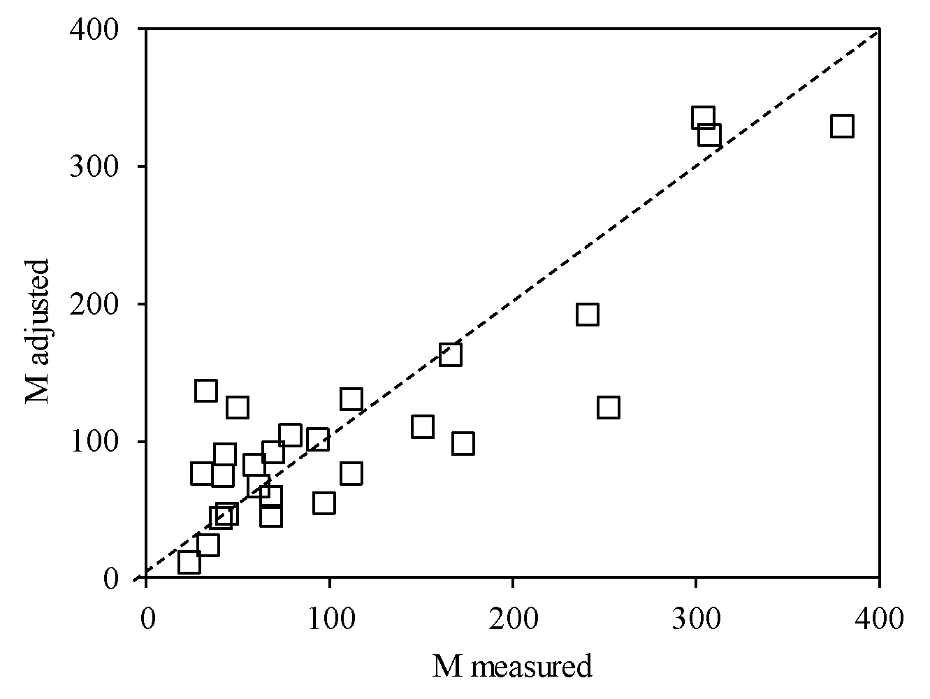
This model is adjusted with an M parameter expressed in mg/m2/hour. Equation (16) includes the DWP, PEEV, and TPH, which are used for adjustment of the M parameter. Figure 10 presents the goodness of fit for the adjustment of the M parameter.
Equation (9) for the shear stress-based model is solved with Δx = 10 m and Δt = 5 s. The range of values for M is between 23 and 380 mg/m2/h.
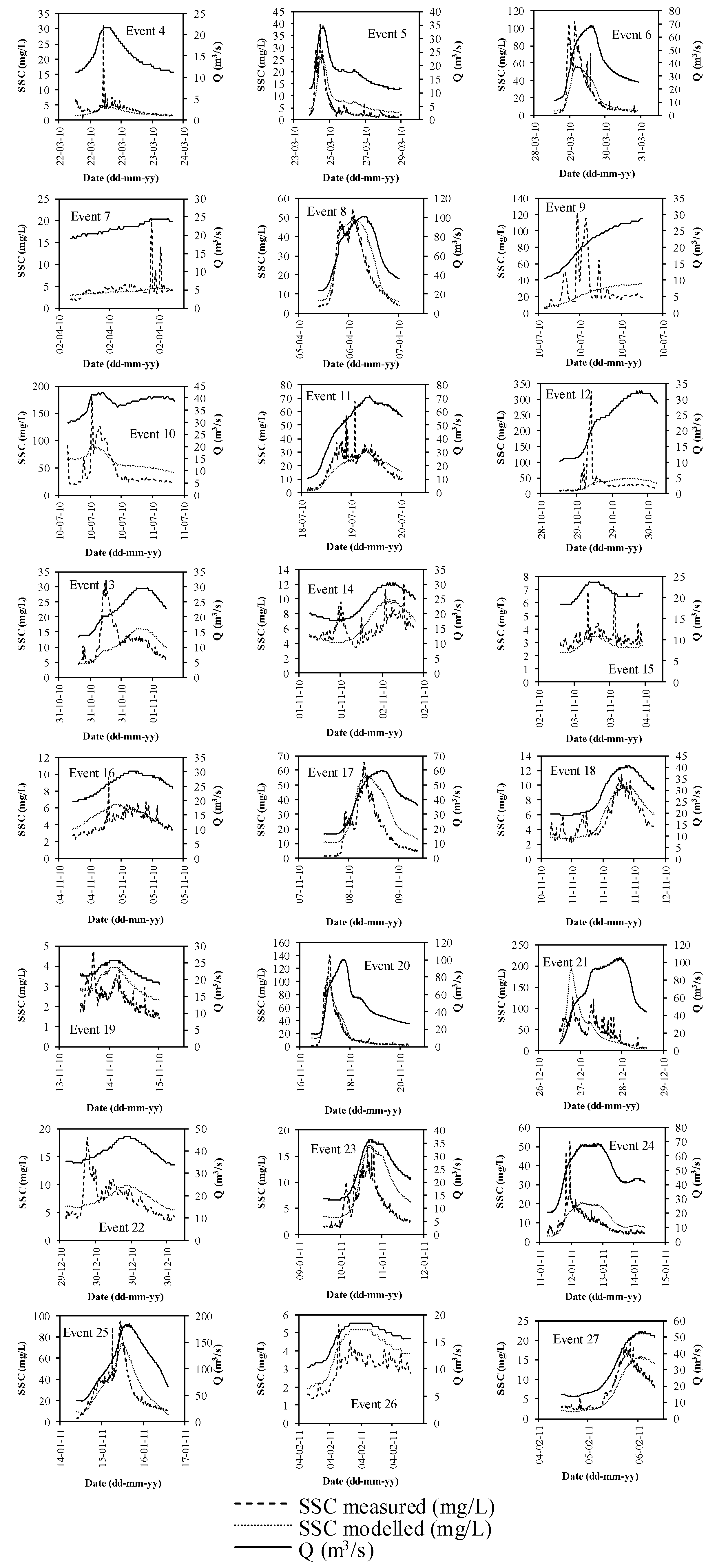
Figure 11 presents the 27 storm events considered, where the measured and calculated SSC values for the shear stress-based model can be observed.
In general, the shear stress model presents outstanding differences to the measured data for most of the storm events analyzed. The SSC curve modeled follows the trend of the shear stress that is proportional to the flowrate of the hydrograph more than the measured SSC. This model requires the inclusion of several additional erosion parameters, instead of just the single M factor. Despite this, for some of the modeled storm events, it can be observed that there is a good agreement, such as for event numbers 2, 5, 6, 7, 18, and 27.
Table 2 summarizes the values of the hydrological and suspended sediment variables obtained for each storm event using the different models presented and applied in this paper.
Table 3 presents the values of the event suspended sediment, ESS, in tons, obtained from the SSCs during the rising (growth) limb of each storm event, and that are used to calculate the uncertainty indices presented below.
The accuracy index, AI; error index, Er; and Nash–Sutcliffe efficiency index, NSE, are calculated according to Equations (17), (18), and (19), respectively, with the results presented in Table 4. The values obtained from the Vansickle and Beschta [2] modified model are less than 15% in the case of the AI index and less than 10% in the case of the Er index. The NSE reaches values higher than 99%. These results provide good agreement.
From the 27 storm events considered, seven of them represent approximately 82% of the total annual fine sediment transported in suspension during storm events. These are also considered as a group and the AI, Er, and NSE indices are also calculated for these seven major events and are presented in Table 4.
According to several watershed studies and suspended sediment simulations, a model simulation can be judged as satisfactory if NSE > 0.50, Er is in the range ±55% for sediment, and AI < 40% [26,27,28].
Here, n is the number of storm events, ESSmeasured and ESScalculated are the total volumes of fine sediment corresponding to each storm event measured and calculated by the three models applied (tons), and is the averaged total volume of fine sediment corresponding to the measured values (tons).
Figure 12 presents the cumulative event suspended sediment, ESS, in tons for the period of study for all 27 storm events. It may be concluded that, in general, all the models proposed at the annual scale are able to reproduce the measured values of SSC for the storm events.
The importance of the present work is based on the recognition that, to model the suspended sediment concentration during different storm events, the following has to be taken into account: the quantity of fine sediments existing in the bed at the initiation of the storm event and how consolidated these sediments are. This is done through the following measurable variables: the existing fine sediment volume stored in the bed, S(t−1); the period between storm events, DWP; and the volume eroded during the previous event, PEEV. The final two variables, DWP and PEEV, were not previously included in the proposed models and constitute a novelty when applying these models. From these variables, the parameters r and M are adjusted in the Vansickle and Beschta [2] and shear stress-based models, respectively. For this paper, the process has been done with the 27 storm events available. In future research work, it is recommended that the calibration of these parameters be reviewed. At this point, the comment of the authors is that to achieve and accurately model the suspended sediment concentration during storm events, it is necessary to consider the parameters mentioned. The advantages of considering the mentioned parameters are: (i) that the model reflects the simulated phenomenon with a greater accuracy when considering the fine sediments in the bed and how consolidated these are, and (ii) the model includes a ‘memory’ from the point of view that previous events influence what will happen next. As the principal disadvantage, we could mention the increase of complexity achieved by the modified proposed model once the parameters r and M are not constant during the storm events values.
4. Conclusions
Three different models have been proposed to estimate the SSC during 27 storm events in a one-year period on the River Bandon, Ireland. The suspended sediment concentration, SSC, during the storm event and total sediment at each event have been compared with measured values.
Uncertainty and error indices have been calculated and values less than 15% and 10%, respectively, have been achieved; this provides good agreement for the Vansickle and Beschta [2] modified model. The NSE index for this model achieves values over 99%.
In the case of the Garcia modified model [3,4], the results are also considered of interest with a NSE value over 94%. The shear stress model needs to include more parameters to improve the modeled data results, which means that the use of this model is not recommended in its current form. More storm events could help to improve the current results.
During the adjustment of the three models, the importance of considering the existing fine sediment volume stored in the bed, S(t−1); the period between storm events, DWP; and the volume eroded during last previous event, PEEV, was identified. These factors are related to the consolidation of the fine sediment in the bed and to the shear stress required to erode such consolidated sediments. The Vansickle and Beschta [2] modified model presents good agreement with measured data and it is recommended that it be used in the study of SSC related to storm events at the Curranure station on the River Bandon.
Author Contributions
J.R.H. planned and developed field measurements and their corresponding quality treatment. J.T.G. and J.R.H. planned the methodology for SSC modeling. J.T.G. analysed and modeled field data. J.T.G. wrote the draft of the manuscript. J.R.H. and J.T.G. reviewed and discussed the results and wrote the final version of the manuscript.
Funding
This research received no external funding.
Acknowledgments
The authors acknowledge the funding received through the Visiting Researchers Programme from the Technical University of Cartagena UPCT, Spain, in the period from August to December 2018. The authors also acknowledge the funding received from the Government of Ireland Technological Research Strand I R&D Skills Programme and the support provided by the Irish Environmental Protection Agency and the Irish Office of Public Works.
Conflicts of Interest
The authors declare no conflicts of interest.
References
- Park, J.; Hunt, J.R. Modeling fine particle dynamics in gravel-bedded streams: Storage and re-suspension of fine particles. Sci. Total Environ. 2018, 634, 1042–1053. [Google Scholar] [CrossRef] [PubMed]
- Vansickle, J.; Beschta, R.L. Supply-based models of suspended sediment transport in streams. Water Resour. Res. 1983, 19, 768–778. [Google Scholar] [CrossRef] [Green Version]
- García, J.T.; Espín-Leal, P.; Vigueras-Rodriguez, A.; Castillo, L.G.; Carrillo, J.M.; Martínez-Solano, P.D.; Nevado-Santos, S. Urban Runoff Characteristics in Combined Sewer Overflows (CSOs): Analysis of Storm Events in Southeastern Spain. Water 2017, 9, 303. [Google Scholar] [CrossRef]
- García, J.T.; Espín-Leal, P.; Vigueras-Rodríguez, A.; Carrillo, J.M.; Castillo, L.G. Synthetic Pollutograph by Prediction Indices: An Evaluation in Several Urban Sub-Catchments. Sustainability 2018, 10, 2634. [Google Scholar] [CrossRef]
- Harrington, J.R.; Harrington, S.T. Sediment and nutrient behaviour on the River Bandon, Ireland. River Basin Manag. 2012, 7, 215–226. [Google Scholar]
- Harrington, S.T.; Harrington, J.R. Dissolved and particulate nutrient transport dynamics of a small Irish catchment: The River Owenabue. Hydrol. Earth Syst. Sci. 2014, 18, 2191–2200. [Google Scholar] [CrossRef]
- Harrington, S.T.; Harrington, J.R. The influence of storm based events on the suspended sediment flux in a small scale river catchment in Ireland. In Monitoring, Simulation, Prevention and Remediation of Dense and Debris Flows IV; WITpress: Southampton, UK, 2012; Volume 4, p. 173. [Google Scholar]
- Harrington, S.T.; Harrington, J.R. An assessment of the suspended sediment rating curve approach for load estimation on the Rivers Bandon and Owenabue, Ireland. Geomorphology 2013, 185, 27–38. [Google Scholar] [CrossRef]
- Krone, R.B. Flume Studies of the Transport of Sediment in Estuarial Shoaling Processes, Final Report, Hydraul; Engineering Laboratory and Sanitary Engineering Research Laboratory, University of California: Berkeley, CA, USA, 1962. [Google Scholar]
- Partheniades, E. A Study of Erosion and Deposition of Cohesive Soils in Salt Water; University of California: Berkeley, CA, USA, 1965. [Google Scholar]
- Park, J. Coupling fine particle and bedload transport in gravel-bedded streams. UC Berkeley ProQuest ID: Park_berkeley_0028E_15142. Merritt ID: ark:/13030/m58w6hxd. Available online: https://escholarship.org/uc/item/1tc2x1g7 (accessed on 22 July 2019).
- Smith, B.P.G.; Naden, P.S.; Leeks, G.J.L.; Wass, P.D. The influence of storm events on fine sediment transport, erosion and deposition within a reach of the River Swale, Yorkshire, UK. Sci. Total Environ. 2003, 314, 451–474. [Google Scholar] [CrossRef]
- Mathers, K.L.; Rice, S.P.; Wood, P.J. Discharge and suspended sediment time series as controls on fine sediment ingress into gravel river beds. Catena 2019, 173, 253–263. [Google Scholar] [CrossRef]
- Mathers, K.L.; Wood, P.J. Fine sediment deposition and interstitial flow effects on macroinvertebrate community composition within riffle heads and tails. Hydrobiologia 2016, 776, 147–160. [Google Scholar] [CrossRef] [Green Version]
- Zabaleta, A.; Martínez, M.; Uriarte, J.A.; Antigüedad, I. Factors controlling suspended sediment yield during runoff events in small headwater catchments of the Basque Country. Catena 2007, 71, 179–190. [Google Scholar] [CrossRef]
- Merchán, D.; Luquin, E.; Hernández-García, I.; Campo-Bescós, M.A.; Giménez, R.; Casalí, J.; de Lersundi, J.D.V. Dissolved solids and suspended sediment dynamics from five small agricultural watersheds in Navarre, Spain: A 10-year study. Catena 2019, 173, 114–130. [Google Scholar] [CrossRef]
- Rymszewicz, A.; Bruen, M.; O’Sullivan, J.J.; Turner, J.N.; Lawler, D.M.; Harrington, J.R.; Conroy, E.; Kelly-Quinn, M. Modelling spatial and temporal variations of annual suspended sediment yields from small agricultural catchments. Sci. Total Environ. 2018, 619, 672–684. [Google Scholar] [CrossRef] [PubMed]
- Harrington, J.R.; Lomasney, L. Suspended and Bed Sediment Transport in the River Bandon, Ireland. In Proceedings of the Civil Engineering Research Association of Ireland Conference, CERI2018, Dublin, Ireland, 29–30 August 2018; pp. 488–493. [Google Scholar]
- Chow, V.T.; Maidment, D.R.; Mays, L.W. Applied Hydrology; McGraw-Hill: New York, NY, USA, 1988. [Google Scholar]
- Mei, Y.; Anagnostou, E.N. A hydrograph separation method based on information from rainfall and runoff records. J. Hydrol. 2015, 523, 636–649. [Google Scholar] [CrossRef]
- Khanal, P.C. Development of Regional Synthetic Unit Hydrograph for Texas Watersheds. Doctoral Dissertation, Lamar University-Beaumont, Beaumont, TX, USA, 2004. [Google Scholar]
- Gamble, J.; Harrington, J.R. Sediment Transport Modelling on the River Bandon. In Proceedings of the Civil Engineering Research Association of Ireland Conference, CERI2016, NUI Galway, Ireland, 29–30 August 2016; pp. 631–636. [Google Scholar]
- Einstein, H.A. The Bed-Load Function for Sediment Transportation in Open Channel Flows (No. 1488-2016-124615); United States Department of Agriculture: Washington, DC, USA, 1950.
- Pochai, N. Numerical treatment of a modified MacCormack scheme in a nondimensional form of the water quality models in a nonuniform flow stream. J. Appl. Mathemat. 2014, 2014. [Google Scholar] [CrossRef]
- Julien, P.Y. River Mechanics; Cambridge University Press: New York, NY, USA, 2018. [Google Scholar]
- Moriasi, D.N.; Arnold, J.G.; Van Liew, M.W.; Bingner, R.L.; Harmel, R.D.; Veith, T.L. Model evaluation guidelines for systematic quantification of accuracy in watershed simulations. Trans. ASABE 2007, 50, 885–900. [Google Scholar] [CrossRef]
- McCuen, R.H.; Knight, Z.; Cutter, A.G. Evaluation of the Nash–Sutcliffe efficiency index. J. Hydrol. Eng. 2006, 11, 597–602. [Google Scholar] [CrossRef]
- Krause, P.; Boyle, D.P.; Bäse, F. Comparison of different efficiency criteria for hydrological model assessment. Adv. Geosci. 2005, 5, 89–97. [Google Scholar] [CrossRef] [Green Version]
Figure 1.
The River Bandon catchment and location of the Curranure gauging station.

Figure 2.
Flowrate and suspended sediment concentration values over the study period on the River Bandon (10 February 2010 to 9 February 2011).
Figure 2.
Flowrate and suspended sediment concentration values over the study period on the River Bandon (10 February 2010 to 9 February 2011).

Figure 3.
Flow rates of the 27 storm-based events modeled to calculate the suspended sediment concentration (SSC).
Figure 3.
Flow rates of the 27 storm-based events modeled to calculate the suspended sediment concentration (SSC).

Figure 4.
Methodology proposed to calculate the suspended sediment concentration, SSC, during a flood event (Garcia et al. [3,4]).

Figure 5.
Adjustment of the r parameter in the Vansickle and Beschta [2] modified model.
Figure 5.
Adjustment of the r parameter in the Vansickle and Beschta [2] modified model.

Figure 6.
Measured and modeled suspended sediment concentration (SSC) concentration with the Vansickle and Beschta [2] modified model.
Figure 6.
Measured and modeled suspended sediment concentration (SSC) concentration with the Vansickle and Beschta [2] modified model.


Figure 7.
Adjustment of the maximum concentration (Cmax) parameter in the Garcia et al. [3,4] modified model.

Figure 8.
Goodness of adjustment of the time to peak of the suspended sediment concentration (SSC) measured data (TPE) and time from the peak of the SSC curve to the end of the curve (TDE) in the Garcia et al. [3,4] modified model.

Figure 9.
Suspended sediment concentration (SSC) measured and modeled with the Garcia et al. [2,3] modified model.


Figure 10.
Goodness of adjustment of the erosion rate (M) parameter for the shear stress-based model.
Figure 10.
Goodness of adjustment of the erosion rate (M) parameter for the shear stress-based model.

Figure 11.
Measured and modeled suspended sediment concentration (SSC) concentration for the shear stress-based model.
Figure 11.
Measured and modeled suspended sediment concentration (SSC) concentration for the shear stress-based model.


Figure 12.
Cumulative event suspended sediment (ESS) for the storm events for the study period.


Table 1.
Constants of the Vansickle and Beschta [2] modified model.
Table 1.
Constants of the Vansickle and Beschta [2] modified model.
| Constant | Value |
|---|---|
| Smax | 430 |
| b | 1.7 |
| a | 0.5 |
| p | 0.02 |
Table 2.
Variables applied in the models.
| Event Number | Peak Flow Date & Time | Qmax (m3/s) | Cmax (mg/L) | DWP (day) | PEEV (Tons) | TPH (day) | TPE (day) | TDE (day) |
|---|---|---|---|---|---|---|---|---|
| 1 | 3 March 2010 23:30 | 37.86 | 72.87 | 19.80 | 21.30 | 0.25 | 0.22 | 0.55 |
| 2 | 19 March 2010 2:45 | 28.03 | 23.29 | 14.69 | 30.92 | 0.41 | 0.49 | 0.25 |
| 3 | 20 March 2010 10:45 | 16.20 | 6.42 | 0.80 | 11.31 | 0.53 | 0.43 | 0.08 |
| 4 | 22 March 2010 16:30 | 21.64 | 6.41 | 1.81 | 3.30 | 0.50 | 0.48 | 0.05 |
| 5 | 24 March 2010 15:15 | 33.69 | 34.71 | 1.09 | 2.56 | 0.78 | 0.61 | 0.66 |
| 6 | 30 March 2010 2:45 | 68.50 | 107.61 | 4.42 | 34.63 | 0.92 | 0.46 | 1.28 |
| 7 | 2 April 2010 18:45 | 24.36 | 20.52 | 2.96 | 186.65 | 0.71 | 0.68 | 0.07 |
| 8 | 6 April 2010 19:15 | 100.12 | 54.51 | 3.13 | 3.60 | 0.90 | 0.68 | 0.79 |
| 9 | 10 July 2010 12:15 | 28.80 | 114.45 | 94.24 | 157.36 | 0.49 | 0.22 | 0.27 |
| 10 | 11 July 2010 3:30 | 41.31 | 117.39 | 94.24 | 42.09 | 0.69 | 0.21 | 0.99 |
| 11 | 19 July 2010 8:45 | 70.63 | 70.00 | 6.90 | 19.21 | 1.22 | 0.98 | 1.20 |
| 12 | 29 October 2010 22:15 | 32.01 | 220.09 | 101.66 | 98.43 | 0.91 | 0.35 | 1.02 |
| 13 | 8 November 2010 16:45 | 28.80 | 31.10 | 1.34 | 25.28 | 0.61 | 0.31 | 0.80 |
| 14 | 2 November 2010 6:30 | 28.80 | 8.77 | 0.32 | 19.67 | 0.90 | 0.80 | 0.27 |
| 15 | 3 November 2010 11:15 | 22.30 | 3.23 | 0.64 | 4.88 | 0.52 | 0.59 | 0.20 |
| 16 | 5 November 2010 4:00 | 29.59 | 5.59 | 0.83 | 1.14 | 0.88 | 0.84 | 0.44 |
| 17 | 8 November 2010 17:00 | 60.21 | 65.34 | 2.26 | 3.63 | 1.20 | 0.80 | 0.96 |
| 18 | 11 November 2010 20:00 | 37.86 | 11.43 | 2.00 | 99.53 | 1.11 | 0.93 | 0.27 |
| 19 | 14 November 2010 5:30 | 25.07 | 4.60 | 1.60 | 7.69 | 0.40 | 0.26 | 0.05 |
| 20 | 17 November 2010 19:45 | 98.15 | 130.68 | 2.19 | 0.62 | 1.19 | 0.77 | 1.66 |
| 21 | 28 December 2010 11:30 | 103.06 | 111.78 | 39.21 | 315.48 | 0.88 | 0.73 | 1.44 |
| 22 | 30 December 2010 10:00 | 45.78 | 18.35 | 1.19 | 408.84 | 0.47 | 0.25 | 0.35 |
| 23 | 10 January 2011 17:15 | 36.18 | 15.43 | 10.35 | 11.98 | 0.94 | 1.02 | 0.24 |
| 24 | 12 January 2011 22:45 | 68.50 | 25.95 | 0.99 | 13.13 | 0.89 | 0.73 | 1.42 |
| 25 | 16 January 2011 2:00 | 184.03 | 75.38 | 1.64 | 61.94 | 1.11 | 0.96 | 1.69 |
| 26 | 4 February 2011 14:45 | 18.51 | 5.46 | 19.19 | 361.17 | 0.34 | 0.20 | 0.09 |
| 27 | 6 February 2011 14:00 | 53.39 | 17.40 | 0.71 | 0.88 | 1.26 | 0.94 | 0.70 |
Table 3.
Event suspended sediment, ESS (tons).
| Event Number | Event Suspended Sediment, ESS (Tons) | |||
|---|---|---|---|---|
| Measured | Vansickle [2] | Garcia [3,4] | Shear Stress | |
| 1 | 30.9 | 17.8 | 30.1 | 23.9 |
| 2 | 11.3 | 8.2 | 21.3 | 11.1 |
| 3 | 3.3 | 2.6 | 5.3 | 1.0 |
| 4 | 2.6 | 1.2 | 8.5 | 3.2 |
| 5 | 34.6 | 29.6 | 24.8 | 17.4 |
| 6 | 186.7 | 176.1 | 122.1 | 120.6 |
| 7 | 3.6 | 2.4 | 8.3 | 5.4 |
| 8 | 157.4 | 181.9 | 86.1 | 327.5 |
| 9 | 23.9 | 20.7 | 45.9 | 23.0 |
| 10 | 43.9 | 47.5 | 35.2 | 48.1 |
| 11 | 98.4 | 81.2 | 141.3 | 101.2 |
| 12 | 62.3 | 69.8 | 25.3 | 65.3 |
| 13 | 19.7 | 15.8 | 11.8 | 13.2 |
| 14 | 4.9 | 7.6 | 19.2 | 8.9 |
| 15 | 1.1 | 0.7 | 6.0 | 6.0 |
| 16 | 3.6 | 4.3 | 18.0 | 13.3 |
| 17 | 99.5 | 134.9 | 81.5 | 48.9 |
| 18 | 7.7 | 8.2 | 7.8 | 9.3 |
| 19 | 0.6 | 1.6 | 5.8 | 15.3 |
| 20 | 315.5 | 313.0 | 277.7 | 200.0 |
| 21 | 408.8 | 396.1 | 470.3 | 558.2 |
| 22 | 12.0 | 9.9 | 13.5 | 5.5 |
| 23 | 13.1 | 16.6 | 4.1 | 19.4 |
| 24 | 61.9 | 72.1 | 116.6 | 216.1 |
| 25 | 361.2 | 371.4 | 313.4 | 123.5 |
| 26 | 0.9 | 1.5 | 2.4 | 1.0 |
| 27 | 26.7 | 24.0 | 29.9 | 31.2 |
Table 4.
Accuracy index (AI), error index (Er), and Nash–Sutcliffe efficiency index (NSE) uncertainty indices.
Table 4.
Accuracy index (AI), error index (Er), and Nash–Sutcliffe efficiency index (NSE) uncertainty indices.
| Index | Model | Calculated Value |
|---|---|---|
| AI (%) all storm events | VanSickle and Beschta [2] modified | 14.2% |
| Garcia et al. [3,4] modified | 40.8% | |
| Shear stress erosion-based model | 101.7% | |
| AI (%) events representing 82% of total storm-suspended sediment transport | VanSickle and Beschta [2] modified | 11.3% |
| Garcia et al. [3,4] modified | 4.17% | |
| Shear stress erosion-based model | 29.6% | |
| Er (%) all storm events | VanSickle and Beschta [2] modified | 9.0% |
| Garcia et al. [3,4] modified | 28.1% | |
| Shear stress erosion-based model | 52.2% | |
| Er (%) Events that represent 82% of total storm-suspended sediment transport | VanSickle and Beschta [2] modified | 6.9% |
| Garcia et al. [3,4] modified | 21.1% | |
| Shear stress erosion-based model | 48.6% | |
| NSE all storm events | VanSickle and Beschta [2] modified | 99.37% |
| Garcia et al. [3,4] modified | 94.69% | |
| Shear stress erosion-based model | 71.29% | |
| NSE events representing 82% of total storm-suspended sediment transport | VanSickle and Beschta [2] modified | 98.33% |
| Garcia et al. [3,4] modified | 88.35% | |
| Shear stress erosion-based model | 42.22% |
© 2019 by the authors. Licensee MDPI, Basel, Switzerland. This article is an open access article distributed under the terms and conditions of the Creative Commons Attribution (CC BY) license (http://creativecommons.org/licenses/by/4.0/).
Share and Cite
MDPI and ACS Style
García, J.T.; Harrington, J.R. Fine Sediment Modeling During Storm-Based Events in the River Bandon, Ireland. Water 2019, 11, 1523. https://doi.org/10.3390/w11071523
AMA Style
García JT, Harrington JR. Fine Sediment Modeling During Storm-Based Events in the River Bandon, Ireland. Water. 2019; 11(7):1523. https://doi.org/10.3390/w11071523
Chicago/Turabian StyleGarcía, Juan T., and Joseph R. Harrington. 2019. "Fine Sediment Modeling During Storm-Based Events in the River Bandon, Ireland" Water 11, no. 7: 1523. https://doi.org/10.3390/w11071523
Note that from the first issue of 2016, this journal uses article numbers instead of page numbers. See further details here.