Article

Data-Driven Approach for Leak Localization in Water Distribution Networks Using Pressure Sensors and Spatial Interpolation

by
Adrià Soldevila
1,†,
Joaquim Blesa
1,2,*,†,
Rosa M. Fernandez-Canti
1,†,
Sebastian Tornil-Sin
1,2,† and
Vicenç Puig
1,2,†
1
Research Center for Supervision, Safety and Automatic Control (CS2AC) Rambla Sant Nebridi, s/n, 08022 Terrassa, Spain
2
Institut de Robòtica i Informàtica Industrial (CSIC-UPC) Carrer Llorens Artigas, 4-6, 08028 Barcelona, Spain
*
Author to whom correspondence should be addressed.
These authors contributed equally to this work.
Water 2019, 11(7), 1500; https://doi.org/10.3390/w11071500
Submission received: 10 June 2019 / Revised: 1 July 2019 / Accepted: 13 July 2019 / Published: 19 July 2019
(This article belongs to the Section Urban Water Management)

Abstract

:
This paper presents a new data-driven method for leak localization in water distribution networks. The proposed method relies on the use of available pressure measurements in some selected internal network nodes and on the estimation of the pressure at the remaining nodes using Kriging spatial interpolation. Online leak localization is attained by comparing current pressure values with their reference values. Supported by Kriging; this comparison can be performed for all the network nodes, not only for those equipped with pressure sensors. On the one hand, reference pressure values in all nodes are obtained by applying Kriging to measurement data previously recorded under network operation without leaks. On the other hand, current pressure values at all nodes are obtained by applying Kriging to the current measured pressure values. The node that presents the maximum difference (residual) between current and reference pressure values is proposed as a leaky node candidate. Thereafter, a time horizon computation based on Bayesian reasoning is applied to consider the residual time evolution, resulting in an improved leak localization accuracy. As a data-driven approach, the proposed method does not need a hydraulic model; only historical data from normal operation is required. This is an advantage with respect to most data-driven methods that need historical data for the considered leak scenarios. Since, in practice, the obtained leak localization results will strongly depend on the number of available pressure measurements and their location, an optimal sensor placement procedure is also proposed in the paper. Three different case studies illustrate the performance of the proposed methodologies.

1. Introduction

All Water Distribution Networks (WDNs) present water leaks up to some extent. Leaks may involve significant economic costs because of water losses and the efforts required for localizing and repairing the leaks. According to [1], water losses due to leaks could be up to 30 % of the total water amount injected in the WDN. This is an important amount considering that water is a scare resource in many regions in the world.
Most water utilities address the leakage control in a passive way; leaks are repaired only when they are visible. Nowadays, there are acoustic instruments [2] allowing us to localize also non-visible leaks, but their application to a large-scale WDN is very expensive and time-consuming. A standard way to facilitate the leakage control is to partition the network into District Metered Areas (DMAs), where the flow and the pressure at the inlet are monitored [1,3]. In [4,5], empirical mathematical models are introduced to describe the relation between the leakage flow and the pressure at the leak location. Another standard approach is based on the night flow at the DMA entrance since it is when demand is minimal and the leak effect corresponds to a relevant percentage of the total flow [1].
Leak localization methods for WDNs have been a very active area of research these last years  [6]. Ref. [7] review the transient-based leak detection methods. In [8], a method to identify leaks is proposed that uses blind spots and the analysis of acoustic and vibration signals for leak detection [9], while [10] proposes models of buried pipelines to estimate wave velocities. Lastly, machine learning methods have been considered for leak localization. Authors in Ref. [11] have introduced a method that uses Support Vector Machines (SVMs) to analyze data from pressure control sensors of WDN for leak localization and size estimation. k-NN and neuro-fuzzy classifiers for leak localization have been suggested in [12,13,14], respectively. Inverse transient analysis methods analyze the pressure data collected during the transitory occurrence by minimizing the difference between the observed and estimated parameters [15,16]. Refs. [17,18] show that unsteady-state tests can be useful for leak detection and localization. Transient-test-based methodologies rely on transient flow analysis in the frequency domain allowing to extract information from the generated pressure waves.
On the other hand, model-based techniques consider stationary models. One of the first model-based approaches was introduced by [19] which formulates the localization problem in a parameter estimation framework. However, WDN parameter estimation is not easy because of the non-linear nature of the model and the reduced number of sensors available [20]. As an alternative approach, Ref. [21] proposed a direct method that analyses pressure measurements inside the WDN with a leak sensitivity analysis (Note that with flow measurements, leaks could be more easily located since simple mass balances can be established in the pipes, but pressure sensors are cheaper and easier to install and maintain and are preferred by the water utilities to localize leaks). This methodology uses pressure residuals (defined as differences between measurements of the associated estimations from the WND model) that are obtained on-line. Leak detection is possible by comparing these residuals with some thresholds that consider the modeling uncertainty and noise. If some of the residuals exceed the corresponding threshold, a leak is detected. The leak localization is possible by matching the residuals with the binarized leak sensitivity matrix. However, the performance of this approach is highly affected by nodal demand uncertainty and measurement noise. To improve the results, the analysis of the residuals without binarization is proposed in [22,23] using correlation analyses with the leak sensitivity matrix. Recently, classifiers have been propose to analyse the residuals in [24,25].
In this paper, a new method for leak localization in WDNs is proposed. It is based on three main ideas: (i) Historical data are used consisting in recorded pressure measurements in some internal network nodes, to capture the network normal operation (i.e., reference behaviour); (ii) The Kriging spatial interpolation technique is used to estimate the pressure at the network nodes that are not equipped with sensors; (iii) All network nodes (equipped with pressure sensor or not) are considered in order to point as leaky node the one that presents maximum pressure drop between its reference pressure value and its current (measured or estimated) value. The proposed method presents two interesting properties. First, it is a data-driven method that does not require the construction and difficult calibration of a hydraulic model. Second, it only needs historical data from normal operation behaviour, in contrast to conventional data-driven methods that require historical data for the considered abnormal behaviours. In addition, a sensor placement algorithm is proposed to place a given number of pressure sensors in the network in such a way the leak localization performance is optimized. For the sensor placement procedure, a hydraulic model is used to generate approximate pressure values in the nodes of the WDN.
The rest of the paper is organized as follows. In Section 2, the leak localization problem is introduced and the proposed solution method is presented. In Section 3, an algorithm to determine the optimal location of pressure sensors is proposed. Section 4 illustrates the application of the whole methodology to three different WDNs. Finally, Section 5 draws the main conclusions of the work.

2. Leak Localization

2.1. Assumptions and Basic Operation

The problem of leak localization can be viewed as a particular case of the problem of Fault Detection and Isolation (FDI) widely studied in the literature. A common assumption in FDI is to consider that only one fault (here a leak) can occur at a time. This assumption will also be considered in this paper. Moreover, another well accepted assumption in WDN leak localization is to assume that leaks occur in the WDN nodes (as assumed in [21,26], or [25]), which makes the problem manageable.
Consider a WDN with n n nodes operating with given boundary conditions c established by the internal valves positions, reservoirs pressures, flows and consumer demands. Consider also the presence of a leak l j with magnitude l and acting on node j. From nodal pressure measurements, a residual vector can be created as follows
r = p ( c ) p ( l j ) ( c )
where
  • p ( c ) = p 1 ( c ) , , p n n ( c ) is the pressure map with the WDN with boundary conditions c and leak-free case.
  • p ( l j ) ( c ) = p 1 ( l j ) ( c ) , , p n n ( l j ) ( c ) is the pressure map with the WDN boundary conditions c and a leak scenario in node j with a leak of magnitude l.
The leak localization is achieved by determining the pressure residual component with maximum size (see [27,28]), i.e.,
j ^ = arg max i { 1 , , n n } { r i }
where r i , i = 1 , , n n are the the residual vector components in (1).
In practice, two limitations appear. First, a limited number of network nodes are sensed in real WDNs because of the high cost of pressure sensor installation and maintenance. To consider in which nodes we have a pressure sensor, the following vector is used
q = q 1 , , q n p
where n p is the number of locations where sensors can be installed and components q i are binary values that indicate if a sensor is placed at the node i ( q i = 1 ) or not ( q i = 0 ). The first limitation can be faced by using spatial interpolation techniques which, starting from the available pressure measurements in several network nodes, are able to estimate the pressure in the other nodes.
The second limitation comes from the fact that experimental data for leak-free operation are limited. However, if sensor data under exactly the same operating conditions c are not available, it is possible to consider other close operating conditions c ^ instead. In practice, the global flow consumption and the pressure at the inlets can be measured, but it is not the case of the nodal demands, which are unknown.
Taking into account the two previous limitations, the residual vector (1) can be rewritten as follows
r ^ = p ^ ( c ^ , q ) p ^ ( l j ) ( c , q )
where
  • p ^ ( c ^ , q ) is the pressure map in the WDN with boundary conditions c in a non leak scenario estimated using q sensors. If q i = 1 , it is computed by using pressure recorded values p i ( c ^ ) ; otherwise it is computed by interpolation techniques for estimating the pressure in nodes without sensor.
  • p ^ ( l j ) ( c , q ) is the pressure map in the WDN with boundary conditions c and leak scenario in node j with magnitude l using q sensors. If q i = 1 , it is computed using the measurement values p i ( l j ) ( c ) ; otherwise the pressure values are estimated by means of interpolation techniques.
Leak localization by using the approximated residual vector (4) instead of the ideal residual vector (1) in (2) can be done as follows
j ^ = arg max i { 1 , , n n } { r ^ i }
The leak localization performance of (5) instead of the ideal one in (2) highly depend on the number of sensors, their location in the WDN, and the amount of historical data available from these sensors.

2.2. Pressure Estimation by Means of Interpolation

To compute the approximated residual vector (4), interpolation techniques will be used to estimate the pressure values in nodes without sensors installed.
In this paper, the Kriging approach is the interpolation technique proposed. This technique is a well-known interpolation method in the area of geostatistics, see [29] for a recent review. Kriging relies on predicting the value of a function at a given point by the weighted average of function known values in the neighborhood of this point.
Denoting the unmeasured pressure estimation in a node i as p ^ i ( l j ) ( c , q ) can be obtained using a fitted Kriging model as follows [30]
p ^ i ( l j ) ( c , q ) = μ + ε χ , θ , d i ( q )
where μ represents the interpolation static part and the function ε χ , θ , d i ( q ) is the spatially correlated part. Both terms constant μ and function ε ( · ) are obtained in the fitting process as well as function parameters χ and θ . On the other hand, d i is the i t h row of a symmetric matrix D n n × n n whose components d i , j are the minimum distance in pipe [m] from node i to node j that takes into account the network connectivity and ( q ) denotes that only the components of d i associated to the measured nodes are considered. The fitting process consists in a least square error minimization problem considering available pressure measurements p ( l j ) ( c , q ) and distance matrix D s ( q ) n s × n s which is a submatrix of the matrix D but only considering the distances between the n s sensors. Function ε ( · ) has two parts to be estimated in the fitting process
ε χ , θ , d i ( q ) = λ β f 1 χ , d i ( q ) + γ f 2 θ , d i ( q )
where λ is a scaling factor obtained in the fitting process similarly to μ , f 1 χ , d i ( q ) is a polynomial function, that returns a scalar value, depending on the given d i ( q ) value and χ u where u is the polynomial order plus one, f 2 d i ( q ) , θ is a correlation function which returns a scalar value, that depends on the estimated values θ n s and the given d i ( q ) . Finally, β and γ are estimated constants weighting the polynomial and the correlation functions (for more details see [29]).

2.3. Bayesian Time Reasoning

The leak localization method defined by (5) takes into account only the computation of the residual vector (4) by means of the measurements at the current time instant k. To take into account the time evolution of the residuals, which will result in an improved leak localization accuracy, a Bayesian reasoning strategy is proposed.
The residual vector (4) is updated at each time instant k for every leak node candidate i = 1 , , n n . An offset equal to the minimum component of vector r ^ ( k ) is added to every component at every instant k in order to have only positive values
r ^ i ( + ) ( k ) = r ^ i ( k ) + min r ^ ( k )
Then, a likelihood index α i ( k ) is obtained for every leak node candidate i = 1 , , n n as the normalization of the r ^ i ( + ) ( k ) values as follows,
α i ( k ) = r ^ i ( + ) ( k ) j = 1 n n r ^ j ( + ) ( k )
The α i ( k ) is a measure of which ones of the n n nodes present the most disturbed residuals and therefore allows to identify the candidates to be the leaking node. This information can be combined to the initial leak probabilities for each node P i ( k 1 ) by means of the Bayes rule in order to obtain updated posterior leak probabilities
P i ( k ) = P i ( k 1 ) α i ( k ) j = 1 n n P j ( k 1 ) α j ( k )
Then, the leak node localization can be estimated by using posterior leak probabilities by
j ^ ( k ) = arg max i { 1 , , n n } { P i ( k ) }
instead of evaluating the approximated residual vector in (5).
The starting point can be an unprejudiced one (all nodes are equally probable to be leaky), i.e.,  P i ( k ) = 1 / n n , and as long as new sample measurements are available and the α i ( k ) are computed, the updated values of P i ( k ) allow to proceed to discard many of the candidate leaks.
One drawback of applying (10) to compute posterior probabilities is that if the posterior probability of any of the leaks takes the value of 1 at any time instant k, then all the remaining leaks take the 0 probability value at instant k and future time instants because of the recursive application of (10). To avoid this problem, a term corresponding to the average value of residual vector r ^ ( + ) ( k ) multiplied by a value δ < < 1 is added in the normalization process so that (9) is improved as
α i ( k ) = r ^ i ( + ) ( k ) + δ 1 n n z = 1 n n r ^ z ( + ) ( k ) j = 1 n n r ^ j ( + ) ( k ) + δ 1 n n z = 1 n n r ^ z ( + ) ( k )
This way the maximum value of α i ( k ) at any time instant k is limited to
α m a x ( k ) = 1 δ n n 1 n n z = 1 n n r ^ z ( + ) ( k ) j = 1 n n r ^ j ( + ) ( k ) + δ 1 n n z = 1 n n r ^ z ( + ) ( k )
and the minimum value for α i ( k ) at any time instant k is guaranteed to be at least
α m i n ( k ) = δ 1 n n z = 1 n n r ^ z ( + ) ( k ) j = 1 n n r ^ j ( + ) ( k ) + δ 1 n n z = 1 n n r ^ z ( + ) ( k )
where δ has to be chosen small enough to avoid providing high probability to residuals r ^ i ( + ) close to zero.

2.4. Performance Indicators
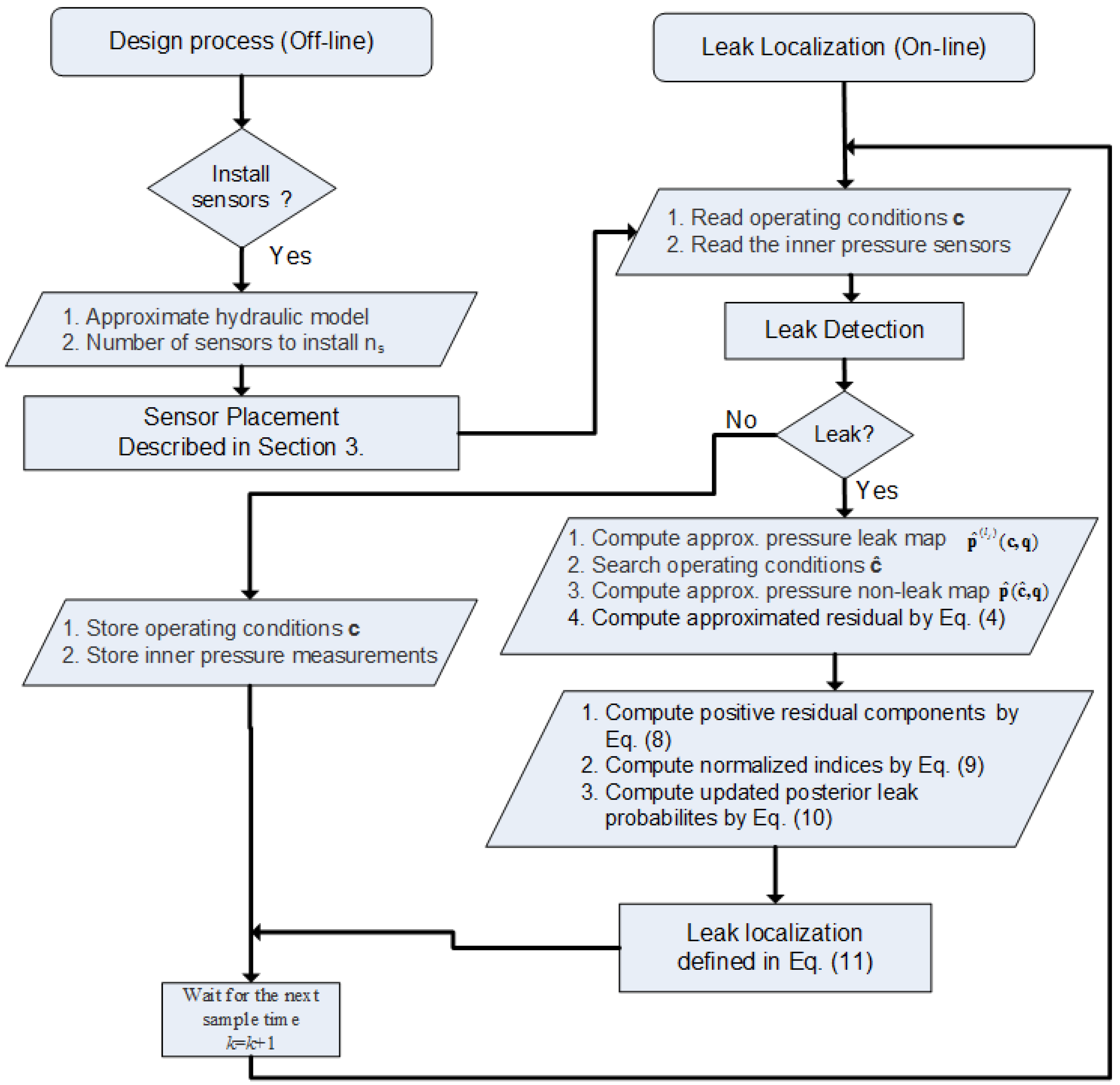
To assess the performance of the leak localization approach defined by (11), the confusion matrix ( n n × n n ) depicted in Table 1 is used. The rows correspond to the leak scenario and the columns to which leak is located ( l ^ ) by the leak localization method.
Considering m V different scenarios for every leak l i i = 1 , , n n , in an ideal case (perfect localization) the confusion matrix should be diagonal, i.e., Γ i , i = m V . However, in a real case, non-zero coefficients will appear outside the main diagonal of matrix Γ . For every leak i, the number of times that the leak l i is correctly identified as l ^ i is indicated by the coefficient Γ i , i , while the number of times that leak i is wrongly identified is indicated by j = 1 n n Γ i , j Γ i , i . The overall accuracy is defined as
Ac = i = 1 n n Γ i , i i = 1 n n j = 1 n n Γ i , j
Since the accuracy value (15) only provides a reference for the perfect leak localization and not how good the leak localization is, in this paper, the Average Topological Distance (ATD) is the indicator used to assess the overall performance as proposed in [24]. The ATD is the average value of the minimum distance in nodes between the node candidate provided by the leak localization method and the actual node with the leak. The ATD is computed as follows
ATD = i = 1 n n j = 1 n n Γ i , j A i , j i = 1 n n j = 1 n n Γ i , j
where A n n × n n is a symmetric matrix such that each element A i , j contains the minimum topological distance (in nodes) between the nodes i and j.

2.5. Summary

The application of the methodology comprises both off-line and on-line stages. The off-line stage is limited to the application of the sensor location algorithm (presented in the next section) for determining the optimal location of a given number of pressure sensors to be installed in internal network nodes. At the on-line stage, at each discrete-time instant k, some main steps are implemented. First, the current operating conditions and internal pressures are determined. If the leak detection module (the implementation of this module is out of the scope of this paper) determines that the network is not affected by any leak, then the current operating conditions and internal pressure values are used to update a database that stores an always up-to-date historical normal operation dataset. On the other hand, if the fault detection module indicates the presence of a leak, then the leak localization procedure detailed in the previous subsections is triggered:
  • Look for the most recent available leak-free historical data captured under similar operating conditions, i.e., at the same hour of the day and with similar input pressure and flow conditions.
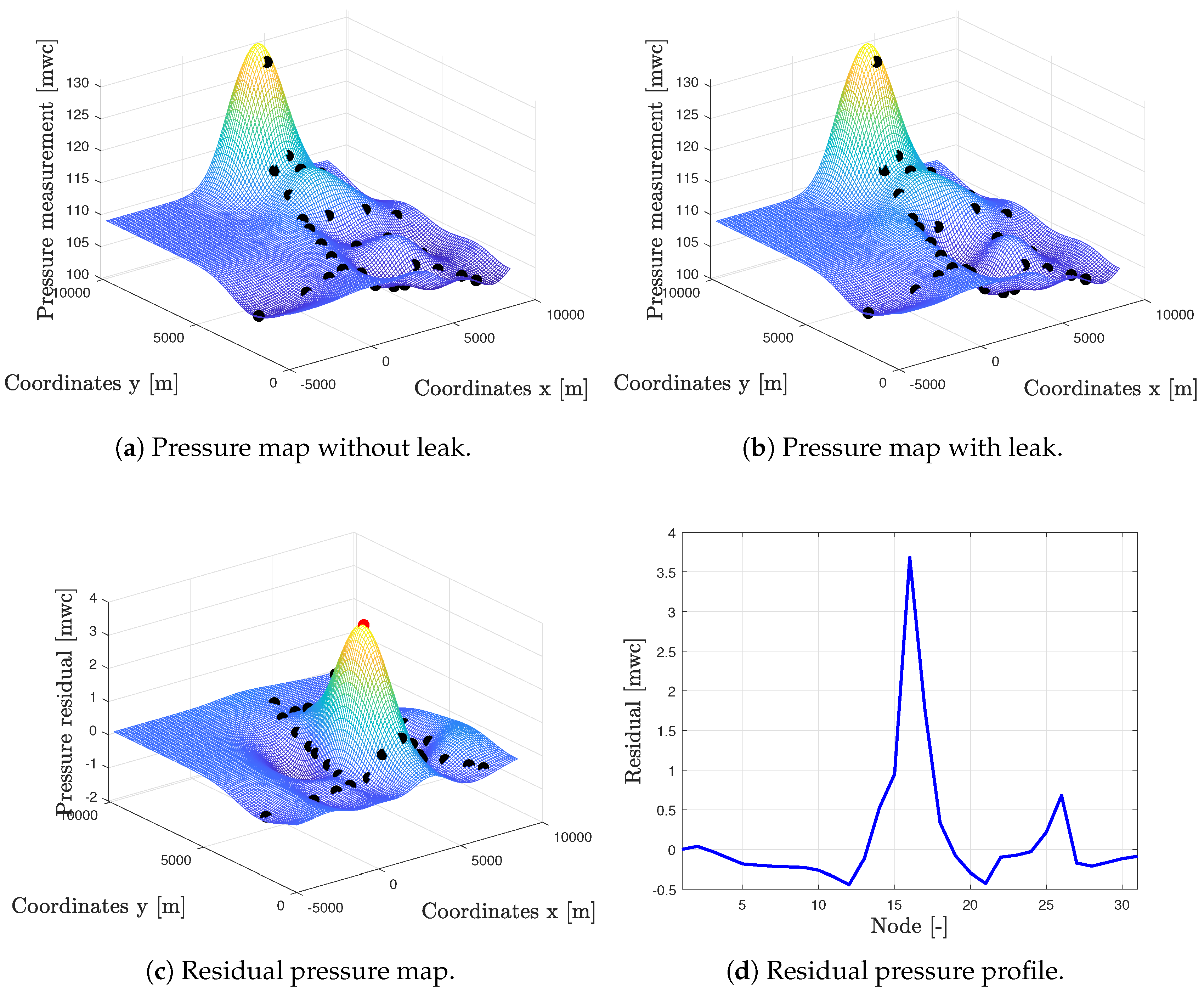
  • Apply Kriging spatial interpolation (6) to the selected historical values to obtain the reference pressure map, i.e., a map containing the reference pressure values for all the network nodes.
  • Apply Kriging (6) to the measured values to obtain the current pressure map.
  • Compare the current and the reference pressure maps by computing the residual (4).
  • Identify the leaky node as the one with greatest difference between pressure maps by using (5).
  • Integrate the individual diagnosis in a time horizon scheme to improve the performance by means of the Bayes rule (10).
The whole procedure is summarized in the flowchart presented in Figure 1.

3. Sensor Placement

The main limitation of the leak localization method based on (5) is that only the pressure measurements of some nodes are available. Therefore, actual values in non-measured nodes are not known and they are estimated by the Kriging method instead. Consequently, the selection of the nodes where the sensors will be installed is a key point to obtain a high performance in the proposed leak localization method.
Given a fixed number n s of sensors to be placed in a WDN, the optimal sensor placement can be formulated as an optimization problem with binary decision variables as follows
min q e ( q ) s . t . i = 1 n p q i = n s
where q is the binary vector that characterizes the locations of the sensors (defined in Section 2.1) and e is a cost function to be minimized. The global solution of the optimization problem (17) would be trivial if all sensor combinations could be evaluated. But, in a real WDN this is not possible due to the large number of nodes. Thus, efficient sensor placement in WDN is an active research area. Sensor placement in WDN was initially focused on water quality monitoring and it is still an active area of research [31,32,33]. Nevertheless in the last years some sensor placement methodologies for leak localization purposes have been proposed as e.g., in [34], where an entropy-based approach was proposed, in [35], where an efficient branch and bound search is used, in [36,37,38], where Genetic Algorithms are used, in [39], where a prior clustering process is applied and in [40] where the sensor placement was formulated as an hybrid feature selection problem.
In general, a given sensor placement method is designed for a particular leak localization method, since there is not a unique optimal set of sensors for a given network (a set of sensors can be optimal for a given leak localization method but not for a different one). In this paper, the sum of square relative errors of the Kriging interpolation in pressure values is used as cost function e considering no-leak and leak scenarios under different boundary conditions c ( k j ) and computed as
e ( q ) = j = 0 n n k j = 1 N j i = 1 n n p i ( l j ) c ( k j ) p ^ i ( l j ) c ( k j ) , q p i ( l j ) c ( k j ) 2
where l 0 denotes no-leak scenario, N j denotes the number of data samples in no-leak scenario ( N 0 ) and in the different leak scenarios ( N j , j 0 ). p ^ i ( l j ) c ( k j ) , q denotes pressure estimations using the sensor configuration defined by q. Since data from all nodes are required, either if they are equipped with a sensor or not, a hydraulic simulator of the WDN can be used to generate data in all the nodes for the different leak scenarios (including the no-leak case) and different boundary conditions ( c ( k j ) ) . In this paper, we will consider the same number of data (boundary conditions) for the no-leak scenario and for all the different leak scenarios N j = N j = 0 , , n n . As a remark, the accuracy of the hydraulic simulator necessary to generate the data for the sensor placement problem is not as critical as if the hydraulic simulator was used in a model-based leak localization scheme. The purpose of the hydraulic simulator that generates pressure values in (18) is to have an idea about the pressure map in the WDN in order to determine the optimal placement for the pressure sensors by means of the optimization problem (17).
In this paper, the Sequential Forward Floating Search (SFFS) algorithm presented in [41] is proposed to solve the optimization problem (17) in a suboptimal but efficient way. The particularization of this algorithm to solve the optimization problem (17) with cost function (18) is described in Algorithm  1.
This algorithm requires the number of sensors to be installed n s and a matrix T where pressure simulation values p i ( l j ) c ( k j ) i = 1 , , n n , j = 0 , , n n and k j = 0 , , N are stored. The pressure data is arranged such that T n n × m T where the n n columns are the pressure values in different nodes and the m T = ( n n + 1 ) N rows represent the different leak scenarios and boundary conditions. On the other hand, the algorithm returns a binary matrix Q ( H ) { 0 , 1 } n s × { 0 , 1 } n f that stores the optimal configurations for an incremental number of sensors n s p = 1 , , n s in its rows q n s p ( H ) { 0 , 1 } n f .
First, the variable corresponding to the number of sensors already placed n s p is initialized to 0 (line 1), the binary matrix Q ( H ) is set to zero and a vector e ( H ) n s p whose components e n s p will store the cost function associated with sensor configuration q n s p ( H ) is also set to zero. In addition, an auxiliary vector q { 0 , 1 } n f to store a sensor configuration is initialized to zero (no sensor selected). Then, the algorithm to place a given number of sensors is executed (lines 2–47) until n s p = n s . The algorithm is divided in two parts: the forward part and the backward part.
Algorithm 1 Sequential forward floating search for sensor placement.
Require: 
The number of sensor to place n s , distance matrix D, training data set T and the number of samples in the training data set m T .
Ensure: 
Suboptimal sensor placement for multiple number of sensors starting from 1 and ending in n s in matrix Q ( H ) .
1:
n s p = 0 , Q ( H ) = 0 , q = 0 , e ( H ) = 0
2:
while n s p < n s do
3:
for i = 1 , , n p do
4:
   e i = 0
5:
   if q i = 0 then
6:
    q i = 1
7:
    for z = 1 , , m T do
8:
     p = t z
9:
     p ^ = Kriging ( q , t z , D )
10:
     e i = e i + j = 1 n n ( p j p ^ j p j ) 2
11:
    end for
12:
    q i = 0
13:
   else
14:
    e i =
15:
   end if
16:
end for
17:
s = argmin ( e )
18:
q s = 1
19:
n s p = n s p + 1
20:
q n s p ( H ) = q
21:
e n s p ( H ) = min ( e )
22:
while n s p > 2 do
23:
   for i = 1 , , n p do
24:
    e i = 0
25:
    if q i = 1 then
26:
     q i = 0
27:
     for z = 1 , , m T do
28:
      p = t z
29:
      p ^ = Kriging ( q , t z , D )
30:
      e i = e i + j = 1 n n ( p j p ^ j p j ) 2
31:
     end for
32:
     q i = 1
33:
    else
34:
     e i =
35:
    end if
36:
   end for
37:
   if e n s p 1 ( H ) > min ( e ) then
38:
    s = argmin ( e )
39:
    q s = 0
40:
    q n s p 1 ( H ) = q
41:
    e n s p 1 ( H ) = min ( e )
42:
    n s p = n s p 1
43:
   else
44:
    Break while.
45:
   end if
46:
end while
47:
end while
The forward part (lines 3–21) consist in adding a new sensor to the previous selected sensor configuration q that minimizes the cost function (18). For this purpose, a vector e n n stores in its components e i the cost function (18) of the previous sensor configuration after adding sensor i. The computation of the cost function (18) is carried out in lines 7–11 where t z , z = 1 , , m T denotes the z t h row of matrix T and Kriging ( q , t z , D ) denotes the Kriging interpolation for all the pressure values using the measurements and distances associated to variable q as was described in Section 2.2. If sensor i is already placed, the cost function (18) is not computed and the component e i is set to (line 14) in order not to consider this impossible case (adding an existing sensor). Once the n p cost functions corresponding to the different n p possible sensors have been computed, the sensor addition that produces a minimum cost value is selected (lines 17–18) and the sensor combination q is stored in q n s p ( H ) , i.e., n s p t h row of matrix Q ( H ) (line 20). In addition, the value of the cost function of the selected sensor configuration is stored in the component n s p t h of vector e ( H ) (variable e n s p ( H ) in line 21). The main advantage of the forward part is that sensors are added sequentially. Therefore, the computational cost of each forward iteration is linear with the number of potential places to install the sensors n p . However, it is not guaranteed that the obtained solution is the best solution among the all possible sensor combinations. In order to minimize the effect of the suboptimality solution of the forward part, a backward part is added.
The backward part (lines 22–46) consists in given a sensor configuration q with n s p selected sensors, evaluate the different n s p sensor configurations of n s p 1 sensors obtained by subtracting one sensor of the original sensor configuration q. If the cost function of this configuration is smaller than the one stored in e n s p 1 ( H ) , the obtained sensor configuration is stored in ( n s p 1 ) t h row of matrix Q ( H ) (variable q n s p 1 ( H ) in line 41) and the number of selected sensors is set to n s p 1 . The backward part is executed after the forward part if the number of selected sensors is more than 2 and is executed until there is not improvement in the new sensor configurations or the number of sensors becomes smaller or equal to 2.

4. Case Studies

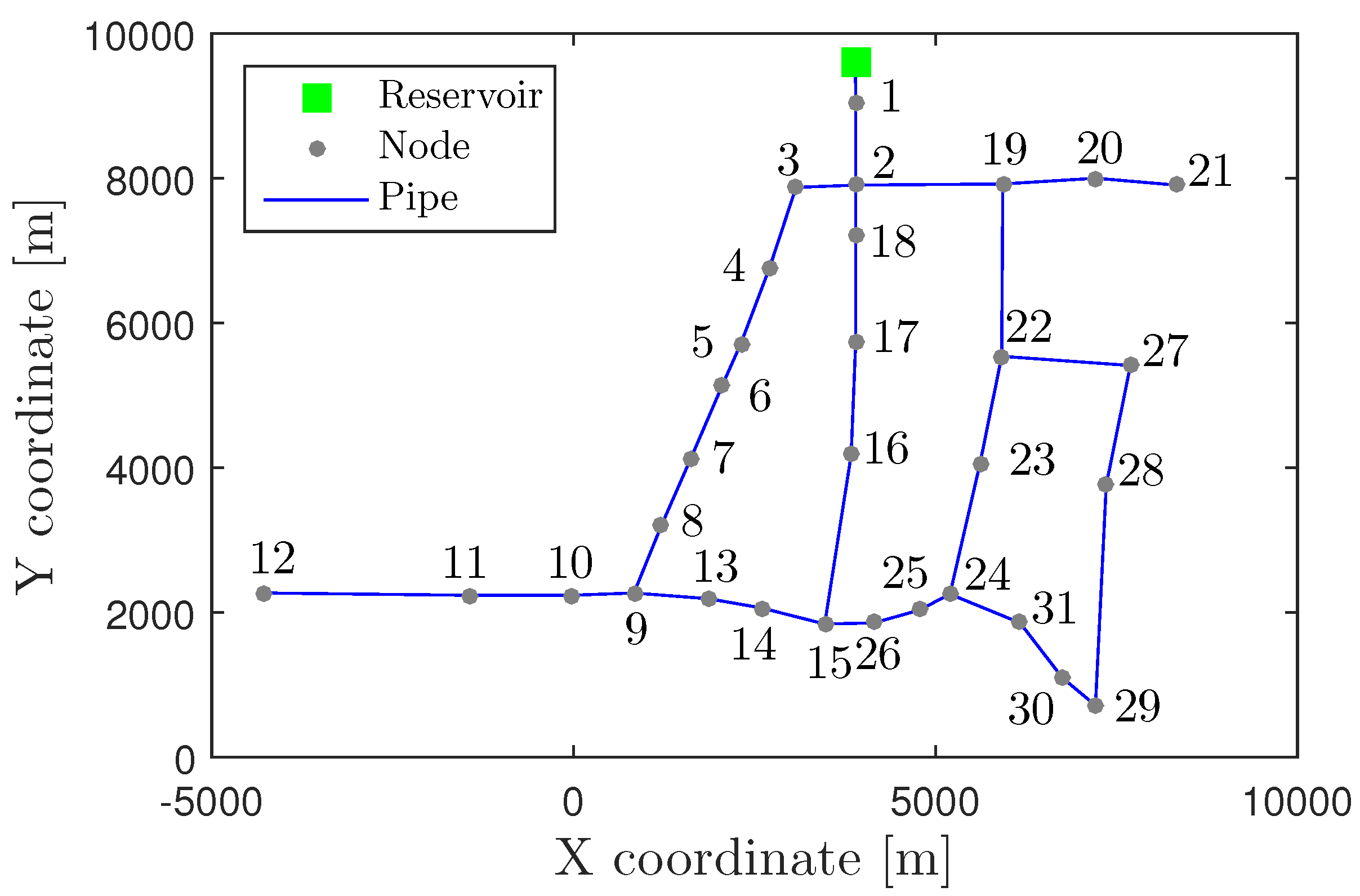
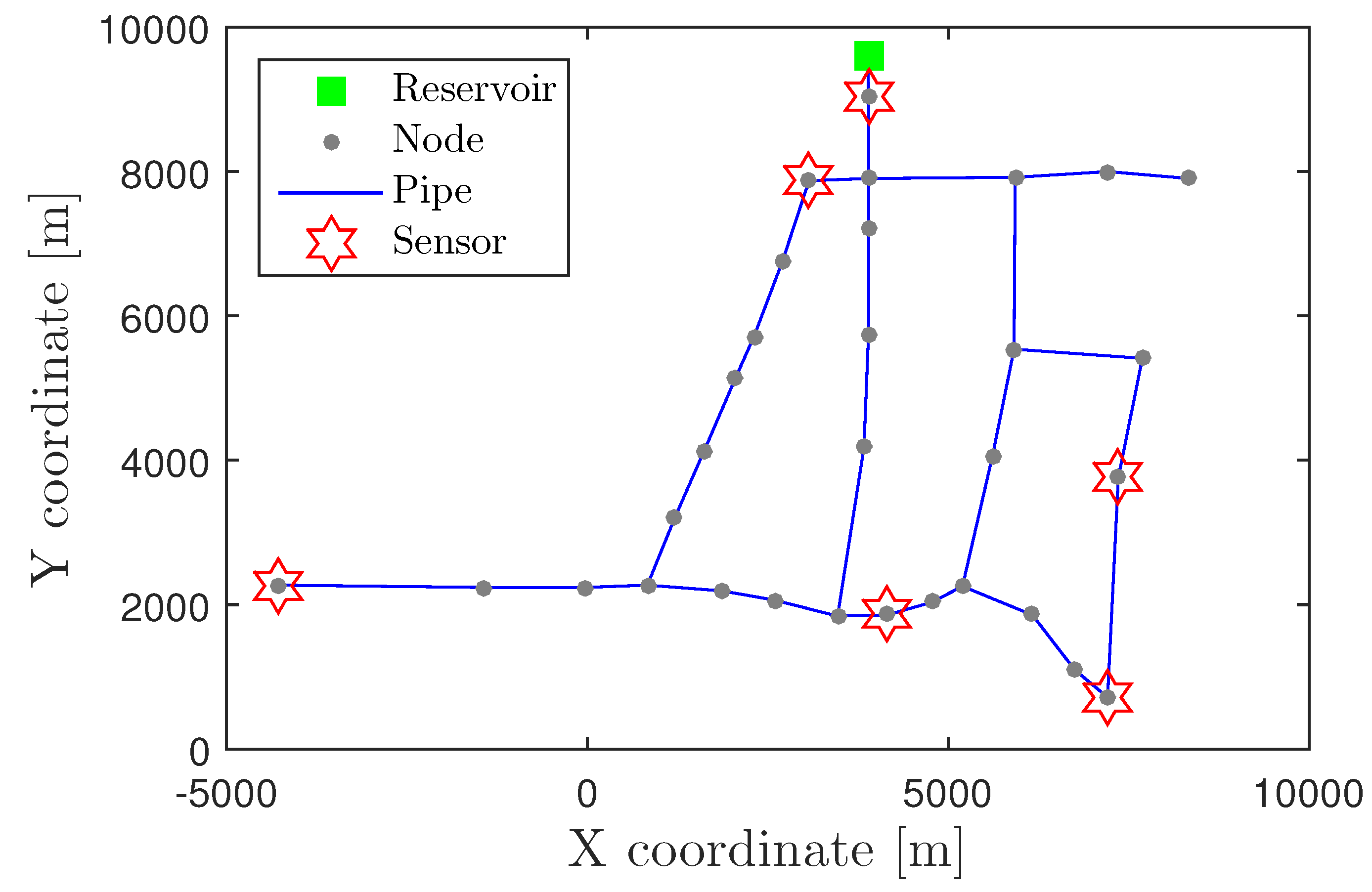
4.1. Hanoi WDN Case Study

The Hanoi WDN is a simplified version of the real WDN from the city of Hanoi (Vietnam), which is composed of one reservoir, 31 consumer nodes and 34 pipes as depicted in Figure 2. The reduced size of this network makes it suitable to illustrate the methods presented in this paper.
The network has an artificially created daily pattern consumption. This daily pattern consumption of water is extracted from the average value of the daily pattern consumption for five days of data from the Nova Icària DMA network, presented later, and adapted (scaled) to the consumption levels of this network. In order to have different daily consumption patterns bounded Gaussian noise is added to the nominal consumption pattern. One example of the daily water consumption pattern artificially generated for this network is presented in Figure 3. Since there is not a pressure valve to regulate the pressure after the reservoir, this is considered constant.
In this network, artificial data is created under different conditions using a hydraulic simulator (Epanet 2, see details in [42]) to test the assessment of the proposed leak localization and sensor placement methods.
Using the hydraulic simulator, data with uncertainties related to the nodal consumer demand, leak size and noise in the measurements are created. The later two by using white noise, while the demand uncertainty is created applying Gaussian noise to the nominal nodal demand, the default valued from the Hanoi benchmark in the Epanet repository, but maintaining the same global consumption (for more details see [43]). In particular:
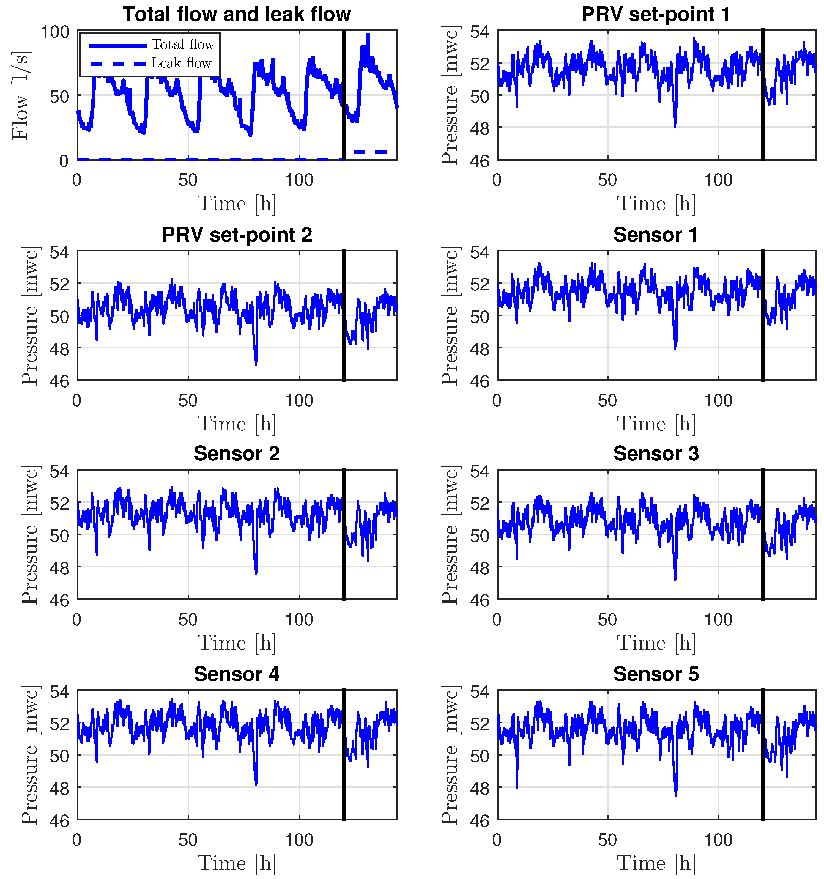
  • The leak uncertainty is taken into account by considering that the exact leak size is not known but it is contained in the range of 25 and 75 [ L / s ] .
  • The noise in the measurements is emulated by adding white noise of the amplitude of 0.1 (zero mean) meter water column ( [ mwc ] ).
  • The demand uncertainty is considered by introducing an uncertainty of the 10 [ % ] of the nominal demand value.
The sampling rate is 10 min, but the measurements at each hour are averaged to reduce the impact of the uncertainties in the diagnosis stage.

4.1.1. Leak localization Assessment in the Ideal Case

In order to illustrate the performance of the leak localization method, first an ideal case considering that all the pressure nodes in (2) are measured is presented. The fault sensitivity matrix approximated by primary residuals has been computed as ([23] for more details)
Ω 1 f 0 r ^ ( l 1 ) , , r ^ ( l n n )
where r ^ ( l j ) is the estimated residual considering a leak in the node j with magnitude f 0 , i.e., computed by (1) considering l j of magnitude f 0 and computed using the hydraulic simulator. In Figure 4, a normalized sensitivity matrix considering r ^ ( l j ) m a x ( r ^ ( l j ) ) instead of r ^ ( l j ) for a leak of 100 [ L / s ] is depicted. As it can be observed, the maximum value (that due to the normalization is 1) is in the diagonal of the matrix. This justifies the use of (1)–(2) and it illustrates that a perfect leak localization is obtained when all network nodes are equipped with sensors.
A particular case can be seen in the Figure 5.

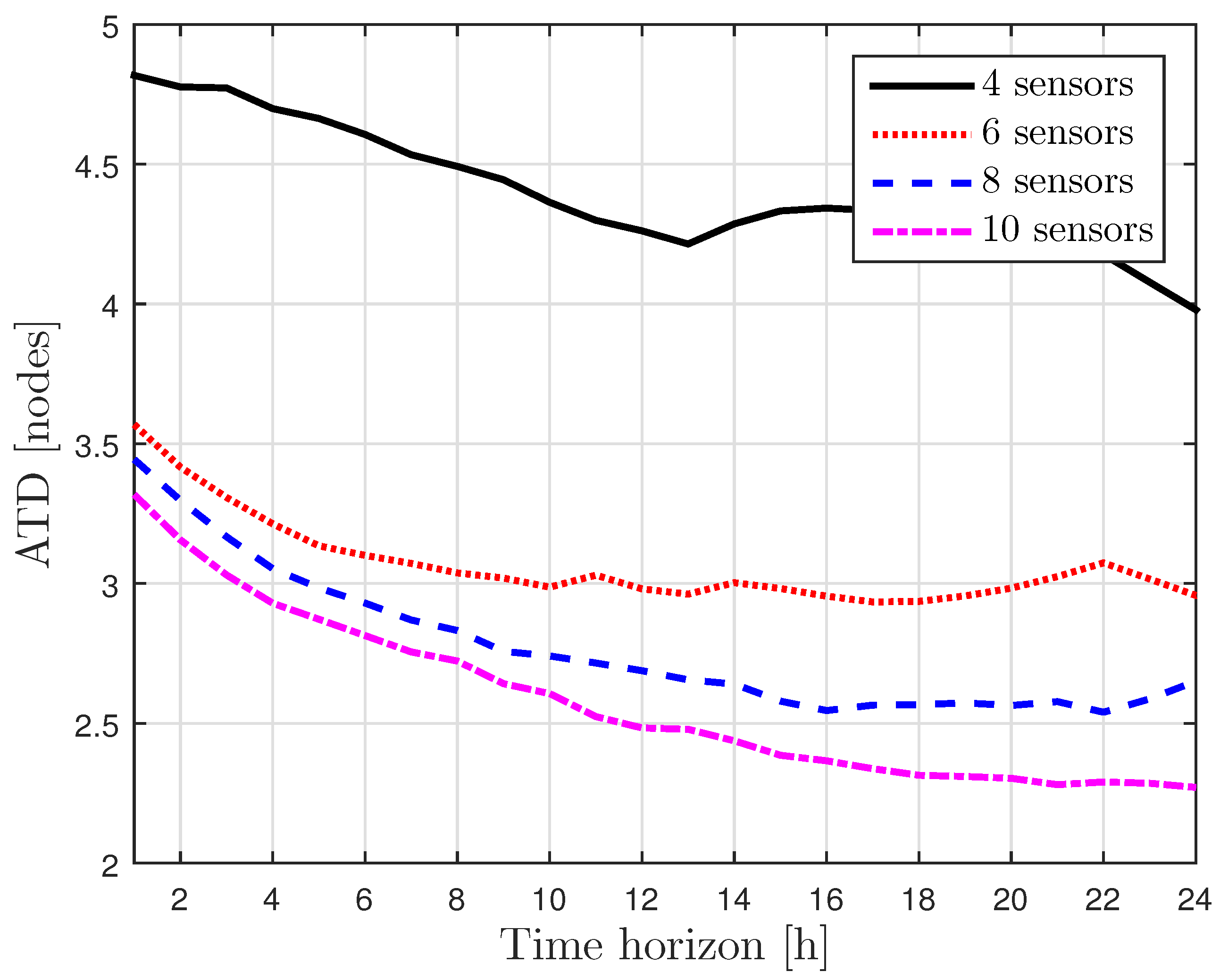
4.1.2. Sensor Placement

In order to consider a more realistic scenario, the sensor placement approach proposed in Section 3 is applied to the Hanoi network, where all the nodes are potential places to install sensors ( n p = n n = 31 ), considering n s = 31 in order to evaluate all the sensor configurations to assess the appropriate number of sensors to install. Artificial pressure data are generated from the hydraulic simulator. In particular, four days of data of no leak scenario and four more days of data for every leak scenario i.e., N = 24 × 4 = 96 has been considered for each scenario. This data has been arranged in a matrix T R n n × m T with n n = 31 and m T = ( 31 + 1 ) × 96 = 3072 since the flow at the entrance of the DMA is considered too. Algorithm 1 proposed in Section 3 has been applied for the number of sensors n s = 31 providing the results for all the suboptimal sensor configurations in matrix Q ( H ) . Kriging interpolation for non-measured nodes proposed in Section 2.2 has been implemented by means of the DACE Matlab toolbox [30]. Once the different suboptimal sensor configurations have been obtained the performance of the leak localization method defined in (5) and by using Bayesian time reasoning (10) is evaluated.
To identify the best historical pressure map p ^ ( c ^ , q ) for a given operational conditions c, past measurements collected at the same hour are used to try to catch the daily routine consumption of water to try to minimize the nodal demand differences, which are unknown. From these measurements, the ones with closest global consumption with respect to the actual measurements are used.
Figure 6 shows the evolution of the ATD as defined in (16) for four different sensor configurations stored in matrix Q ( H ) : four sensors ( q 4 ( H ) ), six sensors ( q 6 ( H ) ), eight sensors ( q 8 ( H ) ) and ten sensors ( q 10 ( H ) ). Regarding the time horizon, the recursive equation (10) is computed before applying leak localization method (11). In this figure, it is shown that leak localization performance improves significatively from four to six sensors but in a more moderate way increasing the number of sensors to eight sensors or ten sensors. The six sensors configuration can be considered the trade-off solution and it is depicted in Figure 7.

4.2. Nova Icària DMA Case Study

The Nova Icària DMA (depicted in Figure 8) is one of the networks inside the Barcelona WDN in Spain. This is a big DMA with two reservoirs, each one with a Pressure Reducing Valve (PRV), 1520 consumer nodes and 1664 pipes. Two flow sensors are placed at the inlets, and five pressure sensors are placed inside the network (the sensor placement of this five sensors is also depicted in Figure 8). All the sensors have a sampling rate of ten minutes and a resolution of 0.1 [ mwc ] . As in the Hanoi case study, here the samples taken inside each hour are averaged to obtain hourly data.
In the Nova Icària network, data from a real leak case have been taken from a test, where a leak was artificially created, in the node with index 996 in the Epanet model, by opening a fire hydrant (the leak size was approximately 5.6 [ L / s ] ). This test was initiated the 20th of December of 2012 at 00:30 am and lasted to the 21st of December of 2012 at 06:30 am approximately (for more details see [23]). Additionally, data of the network without leaks are also available, from the 10th of December of 2012 at 00:00 am to the 14th of December of 2012 at 11:50 pm. The measurements corresponding to the sum of the two DMA inflows and the approximated leak size (is considered constant and equal to 5.6 [ L / s ] ), the pressure reducing valves (PRVs) set-point values in the inlets and the pressure measurements inside the network can be seen in Figure 9 (note that only one day of data with leak is plotted since only this part is used in the leak localization method).
The five days of data without leak are used to create the interpolated maps to be compared with the maps generated with the actual pressure measurements, i.e., to generate the residuals r ^ defined in (4). The result of the leak localization method defined in (11) and using Bayesian time reasoning (10) with one day of the leak data (the first 24 h) provides as the most probable leak node candidate, the node with index 7, which is in a geometric distance of 239.9 m and a topological distance of 23 nodes from the actual leak node. This result is near to the ones obtained by using model-based methods and previously reported in the literature. The correlation method presented in [23] provides as a candidate node the node 1036 with a linear geometric distance of 222.0 m and a topological distance of 17 nodes. The k-NN classifier based method presented in [24] has as candidate node the node 3, with a linear geometric distance of 184.0 m and a topological distance of 13 nodes. Finally, the most recent method tested in this real case, that uses a Bayesian classifier, which is presented in [25], has as candidate node, the node 403 with a linear geometric distance of 183.2 m and a topological distance of 10 nodes. All the candidate nodes for the different methods and the location of the real leak are presented in the Figure 10.

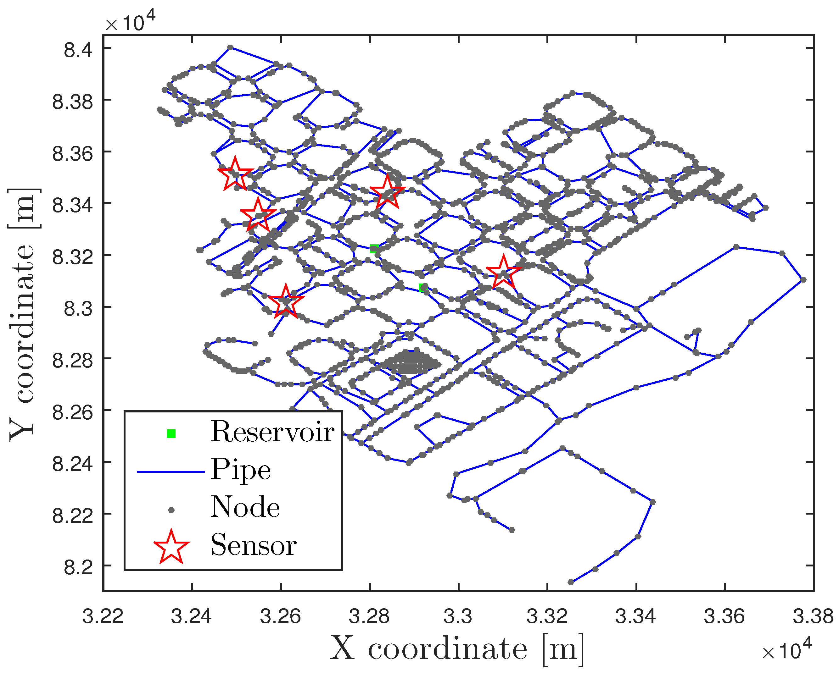
4.3. Madrid DMA Case Study

As second real case study, a DMA of the Madrid network is used. The topology is depicted in Figure 11 and it is composed of one reservoir, 608 demand consumer nodes and 638 pipes. The number of pressure inner sensors is ten, and are placed as depicted in Figure 11. The sampling rate of two minutes, which is the same used for the pressure and flow sensors placed at the inlet. In this network, a leak was artificially created by opening a fire hydrant for a little more than 54 complete hours, and placing a flow sensor (also with a sampling time of two minutes) to record the leak size.
The data from the ten pressure sensors inside the network, and the pressure sensor at the reservoir, before and during the leak, used for the leak localization and the total consumption flow and the leak are depicted in Figure 12.
As proposed earlier, the data are reduced to be hourly by averaging all the samples in each hour. The interpolation is done using the same model adjustment process with data used in the two previous examples. The data used for the training data set corresponds to the measurements taken from the day 25th of November of 2016 at 03:00 pm to the 29th of November of 2016 at 00:58 am. The data record used to do the localization of the leak starts at the 29th of November of 2016 at 04:00 am and finishes the 1st of December of 2016 at 09:58 am (54 h).
The real leak location and the candidate node resulting of the leak localization method defined in (11) and using Bayesian time reasoning (10) recursively during the 54 h are depicted in Figure 13, where the geometric distance between the two nodes is 134 m and the topological distance is 8 nodes.

5. Conclusions

In this paper, a model-free leak localization approach for WDN has been introduced. This approach is based on the particular hydraulic characteristics that appear when a leak in a particular place of the network exists. The Kriging interpolation is used to overcome the problem of a reduced number of sensor measurements in the WDN. The Bayes rule is considered for enhancing the leak localization performance by analysing the residual time evolution. The problem of sensor placement is also addressed, by using a hydraulic model and a feature selection technique with the aim of maximizing the interpolation accuracy.
The performance of the proposed sensor placement is tested in the Hanoi WDN, where the effect of the sensor placement is also evaluated. Moreover, in this network, the proposed leak localization approach is justified by means of artificially injected leaks.
The overall performance of the proposed method for leak localization is assessed for real data in two DMAs in Barcelona and Madrid. In the case of Barcelona, the results are compared to other published methods with satisfactory results.

Author Contributions

All authors have contributed equally.

Funding

This work has been funded by the Ministerio de Economía, Industria y Competitividad (MEICOMP) of the Spanish Government and FEDER through the project DEOCS (ref. DPI2016-76493) and SCAV (ref. DPI2017-88403-R), by MEICOMP and FEDER through the grant IJCI-2014-20801, and by the Catalan Agency for Management of University and Research Grants (AGAUR), the European Social Fund (ESF) and the Secretary of University and Research of the Department of Companies and Knowledge of the Government of Catalonia through the grant FI-DGR 2015 (ref. 2015 FI B 00591) and the Advanced Control Systems (SAC) group grant (2017 SGR 482). The second author acknowledges the support from the Serra Húnter program.

Conflicts of Interest

The authors declare no conflict of interest.

References

  1. Puust, R.; Kapelan, Z.; Savić, D.A.; Koppel, T. A review of methods for leakage management in pipe networks. Urban Water J. 2010, 7, 25–45. [Google Scholar] [CrossRef]
  2. Khulief, Y.; Khalifa, A.; Mansour, R.; Habib, M. Acoustic Detection of Leaks in Water Pipelines Using Measurements inside Pipe. J. Pipeline Syst. Eng. Pract. 2012, 3, 47–54. [Google Scholar] [CrossRef]
  3. Lambert, M.F.; Simpson, A.R.; Vítkovský, J.P.; Wang, X.J.; Lee, P.J. A Review of Leading-edge Leak Detection Techniques for Water Distribution Systems. In Proceedings of the 20th AWA Convention, Perth, Australia, 26–28 September 2003. [Google Scholar]
  4. Lambert, A. What do we know about pressure:leakage relationships in distribution systems? In Proceedings of the IWA Conference System Approach to Leakage Control and Water Distribution System Management, Brno, Czech Rebublic, 16–18 May 2001.
  5. Thornton, J.; Lambert, A. Progress in practical prediction of pressure: leakage, pressure: Burst frequency and pressure: Consumption relationships. In Proceedings of the IWA Special Conference’ Leakage, Halifax, NS, Canada, 12–14 September 2005. [Google Scholar]
  6. Wu, Z.Y.; Sage, P. Water Loss Detection via Genetic Algorithm Optimization-based Model Calibration. In Proceedings of the Systems Analysis Symposium ASCE, Cincinnati, OH, USA, 27–30 August 2006; pp. 1–11. [Google Scholar]
  7. Colombo, A.; Lee, P.; Karney, B. A selective literature review of transient-based leak detection methods. J. Hydro-Environ. Res. 2009, 2, 212–227. [Google Scholar] [CrossRef]
  8. Yang, J.; Wen, Y.; Li, P. Leak location using blind system identification in water distribution pipeline. J. Sound Vib. 2008, 310, 134–148. [Google Scholar] [CrossRef]
  9. Fuchs, H.; Riehle, R. Ten years of experience with leak detection by acoustic signal analysis. Appl. Acoust. 1991, 33, 1–19. [Google Scholar] [CrossRef]
  10. Muggleton, J.; Brennan, M.; Pinnington, R. Wavenumber prediction of waves in buried pipes for water leak detection. J. Sound Vib. 2002, 249, 939–954. [Google Scholar] [CrossRef]
  11. Mashford, J.; de Silva, D.; Marney, D.; Burn, S. An approach to leak detection in pipe networks using analysis of monitored pressure values by support vector machine. In Proceedings of the Third International Conference on Network and System Security, Gold Coast, QLD, Australia, 19–21 June 2009; pp. 534–539. [Google Scholar]
  12. Ferrandez-Gamot, L.; Busson, P.; Blesa, J.; Tornil-Sin, S.; Puig, V.; Duviella, E.; Soldevila, A. Leak Localization in Water Distribution Networks using Pressure Residuals and Classifiers. IFAC-PapersOnLine 2015, 48, 220–225. [Google Scholar] [CrossRef] [Green Version]
  13. Wachla, D.; Przystalka, P.; Moczulski, W. A Method of Leakage Location in Water Distribution Networks using Artificial Neuro-Fuzzy System. IFAC-PapersOnLine 2015, 48, 1216–1223. [Google Scholar] [CrossRef]
  14. Verde, C.; Torres, L. Modeling and Monitoring of Pipelines and Networks: Advanced Tools for Automatic Monitoring and Supervision of Pipelines; Springer: Berlin, Germany, 2017. [Google Scholar]
  15. Covas, D.; Ramos, H. Hydraulic Transients used for Leak Detection in Water Distribution Systems. In Proceedings of the 4th International Conference on Water Pipeline Systems, York, UK, 28–30 March 2001; pp. 227–241. [Google Scholar]
  16. Kepler, A.; Covas, D.; Reis, L. Leak detection by inverse transient analysis in an experimental PVC pipe system. J. Hydroinformatics 2011, 13, 153–166. [Google Scholar]
  17. Ferrante, M.; Brunone, B. Pipe system diagnosis and leak detection by unsteady-state tests. 1. Harmonic analysis. Adv. Water Resour. 2003, 26, 95–105. [Google Scholar] [CrossRef]
  18. Ferrante, M.; Brunone, B. Pipe system diagnosis and leak detection by unsteady-state tests. 2. Wavelet analysis. Adv. Water Resour. 2003, 26, 107–116. [Google Scholar] [CrossRef]
  19. Pudar, R.S.; Liggett, J.A. Leaks in Pipe Networks. J. Hydraul. Eng. 1992, 118, 1031–1046. [Google Scholar] [CrossRef]
  20. Savić, D.Z.; Kapelan, Z.; Jonkergouw, P. Quo vadis water distribution model calibration? Urban Water J. 2009, 6, 3–22. [Google Scholar]
  21. Pérez, R.; Puig, V.; Pascual, J.; Quevedo, J.; Landeros, E.; Peralta, A. Methodology for leakage isolation using pressure sensitivity analysis in water distribution networks. Control. Eng. Pract. 2011, 19, 1157–1167. [Google Scholar] [CrossRef] [Green Version]
  22. Casillas, M.V.; Garza-Castañón, L.; Puig, V. Extended-Horizon Analysis of Pressure Sensitivities for Leak Detection in Water Distribution Networks. In Proceedings of the 8th IFAC Symposium on Fault Detection, Supervision and Safety of Technical Processes, Mexico City, Mexico, 29–31 August 2012; Elsevier: Amsterdam, The Netherlands, 2012; pp. 570–575. [Google Scholar]
  23. Pérez, R.; Sanz, G.; Puig, V.; Quevedo, J.; Nejjari, F.; Meseguer, J.; Cembrano, G.; Mirats, J.; Sarrate, R. Leak Localization in Water Networks. IEEE Control. Syst. Mag. 2014, 34, 24–36. [Google Scholar]
  24. Soldevila, A.; Blesa, J.; Tornil-Sin, S.; Duviella, E.; Fernandez-Canti, R.M.; Puig, V. Leak localization in water distribution networks using a mixed model-based/data-driven approach. Control. Eng. Pract. 2016, 55, 162–173. [Google Scholar] [CrossRef] [Green Version]
  25. Soldevila, A.; Fernandez-Canti, R.M.; Blesa, J.; Tornil-Sin, S.; Puig, V. Leak localization in water distribution networks using Bayesian Classifiers. J. Process Control 2017, 55, 1–9. [Google Scholar] [CrossRef]
  26. Casillas, M.V.; Garza-Castañón, L.E.; Puig, V. Extended-horizon analysis of pressure sensitivities for leak detection in water distribution networks: Application to the Barcelona network. In Proceedings of the 2013 European Control Conference (ECC), Zurich, Switzerland, 17–19 July 2013. [Google Scholar]
  27. Jensen, T.; Kallesøe, C. Application of a Novel Leakage Detection Framework for Municipal Water Supply on AAU Water Supply Lab. In Proceedings of the 2016 3rd Conference on Control and Fault-Tolerant Systems (SysTol), Barcelona, Spain, 7–9 September 2016; pp. 428–433. [Google Scholar]
  28. Romano, M.; Woodward, K.; Kapelan, Z. Statistical Process Control Based System for Approximate Location of Pipe Bursts and Leaks in Water Distribution Systems. Procedia Eng. 2017, 186, 236–243. [Google Scholar] [CrossRef]
  29. Kleijnen, J.P. Regression and Kriging metamodels with their experimental designs in simulation: A review. Eur. J. Oper. Res. 2017, 256, 1–16. [Google Scholar] [CrossRef] [Green Version]
  30. Nielsen, H.B.; Lophaven, S.N.; Søndergaard, J. DACE—A Matlab Kriging Toolbox; Technical University of Denmark: Lyngby, Denmark, 2002. [Google Scholar]
  31. Rico-Ramirez, V.; Frausto-Hernandez, S.; Diwekar, U.M.; Hernandez-Castro, S. Water networks security: A two-stage mixed-integer stochastic program for sensor placement under uncertainty. Comput. Chem. Eng. 2007, 31, 565–573. [Google Scholar] [CrossRef]
  32. Eliades, D.G.; Polycarpou, M.M.; Charalambous, B. A Security-Oriented Manual Quality Sampling Methodology for Water Systems. Water Resour. Manag. 2011, 25, 1219–1228. [Google Scholar] [CrossRef]
  33. Rathi, S.; Gupta, R.; Kamble, S.; Sargaonkar, A. Risk Based Analysis for Contamination Event Selection and Optimal Sensor Placement for Intermittent Water Distribution Network Security. Water Resour. Manag. 2016, 30, 2671–2685. [Google Scholar] [CrossRef]
  34. Christodoulou, S.E.; Gagatsis, A.; Xanthos, S.; Kranioti, S.; Agathokleous, A.; Fragiadakis, M. Entropy-Based Sensor Placement Optimization for Waterloss Detection in Water Distribution Networks. Water Resour. Manag. 2013, 27, 4443–4468. [Google Scholar] [CrossRef]
  35. Sarrate, R.; Blesa, J.; Nejjari, F.; Quevedo, J. Sensor placement for leak detection and location in water distribution networks. Water Sci. Technol. Water Supply 2014, 14, 795–803. [Google Scholar] [CrossRef] [Green Version]
  36. Casillas, M.V.; Puig, V.; Garza-Castañón, L.E.; Rosich, A. Optimal Sensor Placement for Leak Location in Water Distribution Networks Using Genetic Algorithms. Sensors 2013, 13, 14984–15005. [Google Scholar] [CrossRef] [PubMed] [Green Version]
  37. Steffelbauer, D.B.; Fuchs-Hanusch, D. Efficient Sensor Placement for Leak Localization Considering Uncertainties. Water Resour. Manag. 2016, 30, 5517–5533. [Google Scholar] [CrossRef] [Green Version]
  38. Cugueró-Escofet, M.A.; Puig, V.; Quevedo, J. Optimal pressure sensor placement and assessment for leak location using a relaxed isolation index: Application to the Barcelona water network. Control. Eng. Pract. 2017, 63, 1–12. [Google Scholar] [CrossRef] [Green Version]
  39. Blesa, J.; Nejjari, F.; Sarrate, R. Robust sensor placement for leak location: analysis and design. J. Hydroinformatics 2016, 18, 136–148. [Google Scholar] [CrossRef]
  40. Soldevila, A.; Blesa, J.; Tornil-Sin, S.; Fernandez-Canti, R.M.; Puig, V. Sensor placement for classifier-based leak localization in water distribution networks using hybrid feature selection. Comput. Chem. Eng. 2018, 108, 152–162. [Google Scholar] [CrossRef] [Green Version]
  41. Pudil, P.; Novovičová, J.; Kittler, J. Floating search methods in feature selection. Pattern Recognit. Lett. 1994, 15, 1119–1125. [Google Scholar] [CrossRef]
  42. Rossman, L. EPANET 2 User’s Manual; United States Envionmental Protection Agency: Washington, DC, USA, 2000.
  43. Cugueró-Escofet, P.; Blesa, J.; Pérez, R.; Cugueró-Escofet, M.A.; Sanz, G. Assessment of a Leak Localization Algorithm in Water Networks under Demand Uncertainty. IFAC-PapersOnLine 2015, 48, 226–231. [Google Scholar] [CrossRef]
Figure 1. Proposed Method Scheme.
Water 11 01500 g001
Figure 2. Simplified Hanoi topological WDN.
Water 11 01500 g002
Figure 3. Example of a daily flow consumption in the simplified Hanoi topological WDN.
Water 11 01500 g003
Figure 4. Normalized sensitivity matrix of the Hanoi WDN for a leak of 100 [ L / s ] considering all node pressures available.
Water 11 01500 g004
Figure 5. Kriging interpolation for the case of a leak of 100 [ L / s ] at node 16.
Water 11 01500 g005
Figure 6. ATD performance for the sensor placement using different number of sensors in the simplified Hanoi WDN.
Water 11 01500 g006
Figure 7. Sensor placement in the simplified Hanoi topological WDN.
Water 11 01500 g007
Figure 8. Nova Icària DMA topological network.
Water 11 01500 g008
Figure 9. Nova Icària measurements under nominal conditions (before vertical line) and faulty conditions (after vertical line).
Water 11 01500 g009
Figure 10. Nova Icària leak localization results.
Water 11 01500 g010
Figure 11. Madrid DMA topological network and sensor placement.
Water 11 01500 g011
Figure 12. Measurements in the Madrid DMA under nominal conditions (before vertical line) and faulty conditions (after vertical line).
Water 11 01500 g012
Figure 13. Madrid DMA topological network and their sensor placement.
Water 11 01500 g013
Table 1. Confusion matrix Γ .
l ^ 1 l ^ i l ^ n n
l 1 Γ 1 , 1 Γ i , n n Γ 1 , n n
l i Γ i , 1 Γ i , i Γ i , n n
l n n Γ n n , 1 Γ n n , i Γ n n , n n

