Article

Natural Variability and Vertical Land Motion Contributions in the Mediterranean Sea-Level Records over the Last Two Centuries and Projections for 2100

1
Radboud Radio Lab, Department of Astrophysics/IMAPP-Radboud University, P.O. Box 9010, 6500GL Nijmegen, The Netherlands
2
LESIA, Observatoire de Paris, Université PSL, CNRS, Sorbonne Université, Université de Paris, 5 place Jules Janssen, 92195 Meudon, France
3
Istituto Nazionale di Geofisica e Vulcanologia, 00143 Rome, Italy
4
Istituto Nazionale di Geofisica e Vulcanologia, 40100 Bologna, Italy
*
Author to whom correspondence should be addressed.
Water 2019, 11(7), 1480; https://doi.org/10.3390/w11071480
Submission received: 14 June 2019 / Revised: 2 July 2019 / Accepted: 5 July 2019 / Published: 16 July 2019
(This article belongs to the Special Issue Relative Sea-Level Changes and their Impact on Coastal Zones)

Abstract

:
We analyzed a set of geodetic data to investigate the contribution of local factors, namely the sea level natural variability (SLNV) and the vertical land motion (VLM), to the sea-level trend. The SLNV is analyzed through the Empirical Mode Decomposition (EMD) on tidal data (>60 years of recordings) and results are used to evaluate its effects on sea levels. The VLM is measured at a set of continuous GPS (cGPS) stations (>5 years of recordings), located nearby the tide gauges. By combining VLM and SLNV with IPCC-AR5 regional projections of climatic data (Representative Concentration Pathways (RCP) 2.6 and 8.5), we provide relative sea-level rise projections by 2100. Results show that the combined effects of SLNV and VLM are not negligible, contributing between 15% and 65% to the sea-level variability. Expected sea levels for 2100 in the RCP8.5 scenario are between 475 ± 203 (Bakar) and 818 ± 250 mm (Venice). In the Venice Lagoon, the mean land subsidence at 3.3 ± 0.85 mm a−1 (locally up to 8.45 ± 1.69 mm a−1) is driving the local sea-level rise acceleration.

1. Introduction

In situ and remote sensing data show that the rate of global sea-level rise over the past two centuries has increased at faster rates than in the last two or three millennia [1,2,3,4]. Satellite radar altimetry and tide gauge data indicate a rise of the global mean sea-level rate at 1.7 mm a−1 and 3.2 mm a−1 for the 20th century and the last two decades, respectively [5,6,7]. The Mediterranean Sea has been rising at the mean rate of ~1.8 mm a−1 in the last two-three centuries [8,9,10,11,12]. At global scales, the sea-level change is described as the sum of eustatic, glacio-hydro-isostatic, and land-hydrology components [13], which are independently modeled to provide future sea-level predictions. Local sea-level change can significantly differ from mean global sea-level rise because local factors become relevant and their contribution adds up to the global components mentioned above [14]. Oceanographic and climatic effects, glacial isostatic adjustment (GIA), and continuous vertical land motion, especially coastal subsidence due to tectonics (volcanic included) or anthropic origins, are some of the factors that mainly affect sea-level changes at local scales [15]. Therefore, depending on the geographical location they cause spatial variability in the sea-level change pattern. While local effects have little influence at global scale, since they are smoothed out by averaging operations, they become critical in adaptation planning and risk management, where localized assessments are needed.
At time scales of years or decades, oceanographic and climatic factors drive non-stationary sea-level fluctuations, the so-called sea-level natural variability, whose assessment is important for future sea-level projections since their contribution is not negligible [16,17,18,19,20,21,22,23,24,25,26], (http://www.ipcc.ch). For example, in the Indian Ocean the effects of the natural variability, mainly driven by the decadal El Niño–Southern Oscillation (ENSO), Indian Ocean Dipole (IOD) and monsoon, dominate the external forcing contributing up 85% of the observed trend [27]. In the Mediterranean basin, the glacio-isostatic contribution, acting from the Last Glacial Maximum, has a predictable pattern that has been estimated and compared with direct observational data in deforming zones [4,9,15]. The vertical land motion due to natural (tectonics, isostasy and ground compaction) [4,9,13], and/or anthropogenic factors (fluid extraction) [28,29], produces changes in the shape of the basins and changes in the height of the land with respect to the sea (see e.g., [9,13] and references therein). Although this effect does not directly change the quantity of water and its physical properties it results in a net increase (in case of subsidence) or decrease (in case of uplift) of the sea level, when evaluated in restricted geographical areas (as for example the punctual measurements by tide gauges), since the land is moving. If the vertical land motion operates over time it locally results in a net sea-level rate that adds up to the rate induced by GIA, thus affecting the local sea-level change. Tide gauge records are strongly sensitive to the vertical land motion since these instruments are tied to land. Although the role and rates of the main contributors to the sea-level rise are still debated [30], it is a matter of fact that most of the coasts of the world are undergoing the effects of the continuing sea-level rise. The vertical motion due to tectonic effects is strongly variable in the Mediterranean region (as shown in [9] and references therein) and in some areas it can strongly enhance the effect of the sea-level rise. In particular, along subsiding coasts, the rising sea is expected to flood in advance, with respect to stable zones, over the coming decades [1,15,31].
In this framework, the Northern Mediterranean region, being characterized by coastal plains with low elevation (even placed below sea level as some areas of the Adriatic Sea) is therefore prone to marine flooding [9,32,33,34], (www.savemedcoasts.eu), and it represents an interesting case study. Several historical maritime densely-inhabited cities (i.e., Venice and Trieste) and valuable environmental and industrial areas (i.e., Genoa and Marseille) are located in this area. Therefore, detailed studies of local sea-level variations and future projections are relevant to support marine flooding scenarios for a cognizant coastal management.
This study aims to characterize the effect of local factors, such as the sea level natural variability (SLNV) and vertical land motion (VLM), on the sea-level changes at nine locations in the Northern Mediterranean Sea (Figure 1). The SLNV was inferred from tide gauge data through the Empirical Mode Decomposition (EMD) while VLM was measured by means of continuous GPS (cGPS) data. Our approach to estimate SLNV is comprised of two steps: (i) the EMD is applied to tide gauge data to characterize and isolate the natural variability; (ii) a simple theoretical model, based on EMD results, is developed to reproduce the observed SLNV. By combining the SLNV and VLM contributions with the local time-dependent trend based on regional IPCC- fifth Assessment Report (AR5) estimations, the expected sea levels for 2050 and 2100 at each tide gauge location were estimated.

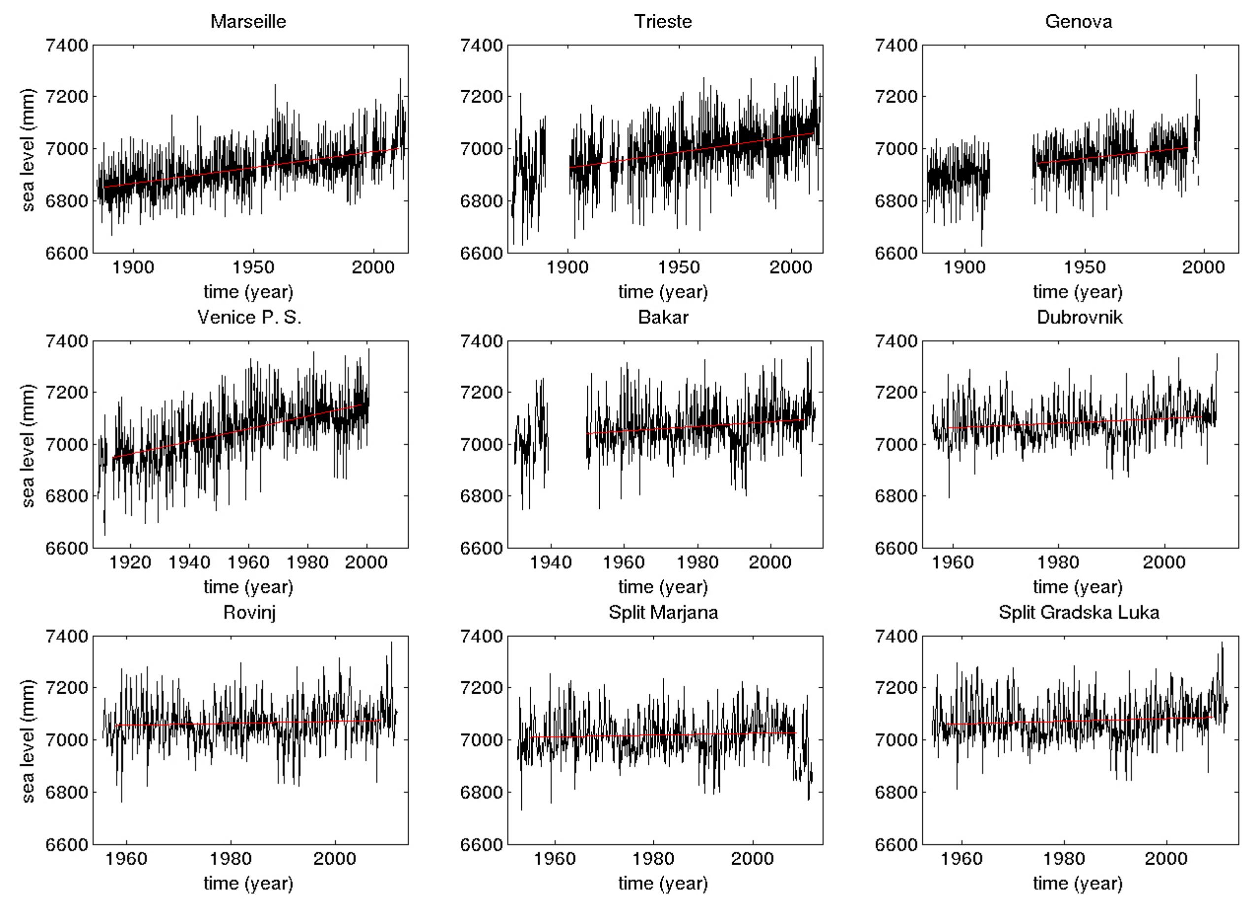
2. Materials and Methods: Data Set and Natural Variability

In this study we analyzed the longest available monthly tide gauge records (>60 years of Revised Local Reference (RLR) data collected in the 1888–2008 time span) at nine tide gauge stations located in the Mediterranean Sea, belonging to the Permanent Service for Mean Sea Level (www.psmsl.org). The location of the stations, the time span of the records and the analyzed time series are shown in Figure 1 and Figure 2. The choice of data sets with length exceeding 60 years aims to avoid the effect of inter-decadal variations affecting tidal recordings shorter than ~50 years [35,36]. In addition, to avoid the introduction of artificial signals in the records, interpolations on data gaps were not applied.
The identification of sea-level trends and large timescales variability from sea-level records is a debated argument and the best methods to discriminate between acceleration and intrinsic climate variability remains an open issue. Indeed, since in tide gauge data the long-term trend is embedded in fluctuations at many different time scales, from daily tides to the seasonal cycle as well as interannual and decadal variations, the filtering method used to remove these variations may impact the accuracy of the calculated trend. Different approaches to this problem have been proposed (for a detailed review see [37]). Among these approaches, the EMD has been used to characterize the intrinsic fluctuations and the long-term trend in sea-level data [38,39,40,41,42,43,44,45]. This technique has been developed to analyze non-stationary and non-linear data, such as tide gauge records, by decomposing the signal in modes that provide a description of the intrinsic timescales present in the time series. Being “adaptive,,” the modes are empirically obtained from the original time series according to its local characteristics. The EMD reveals the proper components of the phenomenon under study better than other methods, such as Fourier analysis, whose modes with predefined functional form are often far from being eigenfunctions of the phenomenon at hand. This makes the EMD very powerful for identifying and isolating, for example, deformed wave profiles, associated with nonlinearities in the data, preserving their local properties. For the applications of this paper, two main reasons guided us in using the EMD. Firstly, the sea level natural variability is described by a few numbers of modes with a quite simple functional form (oscillating functions). This will be exploited in the following for building up a simple low dimensional mode for sea-level estimations. Secondly, the EMD does not require a predetermined timescale to carry out the filtering operation (as it happens e.g., in moving averages commonly used as low-pass filter to recover the large timescale variability in sea-level records): this has an important rational basis, since in a nonstationary process the local timescale is unknown a priori.
In the EMD framework the measured sea level L(t) is decomposed into a finite number n of band-limited oscillating components (called intrinsic mode functions, IMFs) Lj(t), whose functional shape is not fixed a priori, but obtained from the data, and a residue rn(t) providing the nonlinear trend [40]:
  L   t =   j = 0 n L j t +   r n   t .
The procedure of IMF extraction consists of three steps: (i) local maxima and minima of L(t) are identified; (ii) these are connected through a cubic spline identifying the lower and upper envelope; (iii) the signal h(t), the difference between L(t) and the mean of lower and upper envelopes, are calculated. The signal h(t) represents the first IMF, Lj(t), if it has exactly one zero crossing between two consecutive local extrema and its mean is zero. The first condition ensures a global narrowband requirement, namely periods which are too different are not mixed together into an IMF; the second requirement ensures getting oscillations about the zero level. Both these conditions ensure that Lj(t) is an oscillating function with time-dependent amplitude and phase, namely it can be expressed as Lj(t) = Bj(t)cos[ϕj(t)]. If none of these conditions are fulfilled, then step (iii) is repeated by using h(t) as input data. This procedure is iterated until the resulting signal fulfills the IMF properties and it is repeated to find the next IMF by using L(t) − Lj(t) as new input data. When no more modes can be extracted, the difference between the original L(t) and the sum of all IMFs results in the residue rn(t). Technical details on the procedure for IMF extraction are reported in [41]. The EMD allows calculating a meaningful instantaneous phase for each IMF by using the Hilbert transform
L j *   t =   π 1   ×   P   ×   L j   t t t     ×   d t
where P denotes the Cauchy principal value and Lj* represents the complex conjugate of L(t) as ϕj (t) = arctan (Lj*/Lj). Finally, the instantaneous frequency, ωj(t), is given by j(t)/dt. For each Lj(t) we can define a characteristic timescale τj, as the time average <2π/ωj(t)>, that represents an average period of the IMF and provides an estimate of the timescale characterizing the EMD mode. We remark that τj is not to be intended as the Fourier one. It just gives an indication of the timescale characterizing the EMD mode for which it is computed, although many modes with different average periods may contribute to the variability of the actual signal at a particular timescale. The IMF statistical significance with respect to white noise can be evaluated through a test based on the comparison between IMF amplitude from the real signal and from a white noise series [46] at different confidence levels. Since IMFs are a local, complete and orthogonal set, the EMD is useful to filter raw signal through partial sums in Equation (1). Moreover, since a low number of modes are produced, this property can be exploited to build up low order theoretical models to describe the dynamics of the investigated systems.

3. Results: The EMD Analysis and a Generalized Model for Long-Term Sea-Level Variations

When the EMD is used to analyze the nine tide gauge time series, the number of IMFs, n, varies between 10 and 15, depending on the station. This is mainly related to the different lengths of the time series which vary between 137 and 53 years: for the longest time series more components of the natural variability are recovered.
Let S be the set of IMF with timescale >15 years (IMFs timescales τj are shown in Table 1) and significant with respect to a white noise at the 90th significance level. The long-term variations of the measured sea level, LLT, can be defined as:
L L T   t = j ϵ S L j t   +   r n   t ,
where IMFs in S and the residue are added together.
The choice of a 15-year threshold follows the approach used in other studies to remove the short-term variability from sea-level data [1,18]. We remark that, as pointed out by [45], the results of single IMFs from tide gauge data need of a careful interpretation. However, a discussion about the physical meaning of the single IMF is out of the scope of this paper since we use the EMD as a low-pass filter by adding up several IMFs. In this case, the EMD has shown to be a useful tool to reduce the impact of high-frequency variability and noise [45].
The contribution LLT, for the analyzed tide gauges, is shown in Figure 3. All records show a long-term variability in a well-defined range of timescales of about 20–30 and, for the longer records, >45 years, in the typical ranges where internal modes of natural variability are detected [47]. Observational datasets and simulations of the typical scales of Atlantic internal modes of natural variability show variations at decadal timescales that are linked to the ocean-atmosphere coupling [47,48,49,50]. In particular, the 20–30 year variability has been related to the Atlantic Meridional Overturning Circulation (MOC), while the >45 year fluctuations are plausibly due to salinity and matter exchange processes between the Atlantic and Arctic Ocean causing the Atlantic Multidecadal Oscillation (AMO) pattern. Both patterns are quasi-persistent and present up to 8000 years ago [51,52]. The similarity of timescales we found in the tide gauge data with those of the Atlantic modes of variability suggests a connection between climate variability and sea-level variations in the Mediterranean Sea as also indicated by [53,54]. The combined analysis of global oceanic circulation, climate models and observations, indeed, indicates that the main physical mechanism driving the connection between sea level in the Mediterranean Sea and internal modes of natural variability is the mass exchange through the Strait of Gibraltar [53]. This mechanism generates a coherent and uniform signal in the whole Mediterranean at decadal time scales [54,55]. The detected sea-level variations at 20–30 years can be thus related to the combined effect of the North Atlantic Oscillations (NAO) and AMO [26]. An additional contribution could come from the Inter-decadal Pacific Oscillation (IPO), causing variations of the global surface temperature at these timescales, which affects also the climate dynamics in the Atlantic Ocean [56,57]. Likewise, major volcanic eruptions, affecting the global temperature by acting on the radiative forcing [57,58], could also contribute to the SLNV. Fluctuations at longer timescales can be due to both atmospheric forcing [59] and exchange processes [47].
A first check of the EMD results can be performed by comparing the SLNV obtained for the four closest stations in the North Adriatic sea, namely Venice, Trieste, Bakar, and Rovinij that are separated by a minimum and maximum distance of ~65 and ~150 km, respectively. Figure 4 shows a comparison of the EMD reconstructions, through IMF with timescale >15 years (the residue rn(t) has not been added up), for these records. For the four stations the variability is very similar with maxima and minima almost in phase. Small differences can be due to border effects for shorter series (e.g., Rovinij) and/or presence of data gaps affecting the IMF calculation or natural reasons such as small local differences in the signal variability. We note that the Venice station shows a different behavior with a flatter signal between 1945 and 1980 due to temporary anthropogenic subsidence induced by groundwater [28].
Results show that, for all the stations, the SLNV is described by a small number of EMD modes (from 3 to 6). Since IMFs are oscillating functions, we modelled the long-term behavior of the tide gauge signal as the superposition of a linear trend and the sum of oscillating functions of given amplitude, frequency and phase:
L M t =   r t   +   c   +   i = j k A j   ×   cos Ω j t   +   Φ j .
In Equation (4) the trend is linear, and the long-term fluctuations are accounted by oscillating functions whose frequency Ωj is the time average of the instantaneous frequency of IMFs in S. This represents the most elementary approximation to reproduce the long-term variability inferred by the EMD through modes with time-dependent amplitude and phase. The free parameters in Equation (4) (rate r, intercept c, Aj and Φj) are calculated by fitting LM(t) to LLT(t). To avoid possible end effects due to the procedure of IMF extraction and the computation of derivative at borders, we cut three years of data at both boundaries of LLT(t) before performing the fit. In addition, since data from Trieste, Genoa, Venice, and Bakar show gaps in the initial part of their records, for these stations the fit starts from year 1901, 1931, 1914, and 1949, respectively, when recordings begin to be continuous for many decades. Two sources of uncertainty were taken into account. Firstly, the uncertainty due to the use of constant frequencies, instead of time varying ones, is evaluated by building 1000 LM(t) realizations whose j are randomly extracted from a Gaussian distribution with mean < ωj(t) > and standard deviation σ [ωj(t)]. Secondly, effects of possible undetected modes of climate variability, with periods of the order and/or longer than the record lengths, are taken into account as an increase of the estimated uncertainty. Indeed, since these very long period modes are not included in the model, the accuracy for estimating the sea level is reduced. This additional uncertainty is accounted for by adding to each realization LM(t) a normally distributed zero average white noise. Since we expect that modes with periods of the order and/or longer than the record lengths are settled on the EMD nonlinear residue, the standard deviation of the white noise signal was taken as the standard deviation of the EMD residue from which we subtracted a linear trend.
Figure 3 shows the best solutions obtained by fitting LM(t) to LLT(t). Fit parameters and adjusted R-square statistics are shown in Table 2. R-square values close to 1 indicate that a good fit is achieved for the analyzed records. Rates r obtained by a fit through Equation (4) are compatible or slightly higher than rates estimated by a linear fit to the raw data for the same time intervals shown in Figure 2 and varying between 0.35 ± 0.38 mm a−1 (Split M.) and 2.43 ± 0.23 mm a−1 (Venice P.S.). Only for Split Gradska Luka, the linear rate from Equation (4) is higher than the linear fit. This is possibly due to a steeper sea-level rise observed in LLT at this station after 2006. In the raw data, this feature is hidden by short-term fluctuations, thus resulting in a lower rate when a linear fit is computed on the original time series. The origin of this steepening has been proposed to be the coincidence of AMO-NAO phase opposition and warm AMO phase [60]. The same feature is also present in LLT for the Trieste and Rovinj data. However, for Trieste the linear rate from Equation (4) does not show significant differences with respect to the rate of the linear fit likely due to the longer duration of recordings for which the fitting procedure is very robust and not affected by variations in the last part of the data.

4. Discussion: The Vertical Land Motion and Relative Sea Levels by 2050 and 2100

The VLM trends were derived from the processing of raw data collected by regional continuous GPS networks operating in the Euro-Mediterranean region for more than 7 years [61] and located near the tide gauges. The geodetic rates of VLM were obtained from the analysis of position-times series, following the procedures described in [62], according to the IGS recommendations (http://acc.igs.org/reprocess2), to produce solutions with the most updated standards and models. GPS velocities were estimated and represented in the absolute geocentric reference frame (the IGb08 realization of the global ITRF08 [63]. Measured VLM and general information about GPS stations are shown in Figure 5 and Table 3. Due to the poor quality of the data, the VLM at ROGS (Bakar) and RIGS (Rovinj) were not used in this study.
The pattern of vertical GPS rates is variable: the VLM (the average value is considered when more than one cGPS station is available) is almost null in the Gulf of Trieste; it is ≤1 mm a−1 at Marseille, Genova, and Split and it is about 1.5 mm a−1 at Dubrovnik. Sudden temporary tectonic episodes, which can cause permanent signatures during the tidal recordings at these stations, have not occurred (www.psmsl.org).
On the other hand, vertical GPS velocities in the North Adriatic coast around the Venice lagoon, display significant subsidence rates, with values in agreement with previous studies [32,64]. The average VLM in the region, calculated as the average over 14 GPS stations, is −3.30 ± 0.85 mm a−1. Part of the detected subsidence is due to the continuing global glacio-hydroisostatic signal, estimated in this region to be between −0.12 and −0.21 mm a−1 [15], and the remaining part can be related to natural and anthropogenic effects [64,65]. We can reasonably assume that the VLM rate will remain unchanged until 2100 AD, in the absence of additional episodes of land movement that may result from eventual earthquakes with significant magnitude in the area [66] (http://www.isc.ac.uk/). The remarkable subsidence in the Venice lagoon results in a steeper sea-level rate with respect to those provided by IPCC estimations in the area [29,67].
Equation (4) can be used to evaluate sea levels at future times by including both the sea-level trend and VLM, included in r, and the effects of the natural long-term variability, reproduced by the oscillating contributions. By keeping the linear rate derived from a linear fit on the raw data, we implicitly assume a constant trend scenario for which the sea-level trend remains unchanged for the next decades. This represents, of course, a very unlikely scenario since there is high confidence that the rate of sea-level rise is increasing (IPCC – AR5). Therefore, to evaluate more realistic sea levels, a time-dependent rate, obtained from the local IPCC projections and including the VLM contribution is substituted to the constant rate r in Equation (4). Concerning the modeling of the SLNV, since the Atlantic climatic variability is quasi-persistent on secular times [51,52] and since it is connected to the sea-level variations in the Mediterranean sea (see Section 3), we can reasonably assume that the modes of oscillation associated with the natural variability observed in the past, can be considered as reliable for the next ~90 years. The contribution of the natural variability is also significant in a system dominated by a forced CO2 emission, as the Earth nowadays and possibly in future years. Studies on the effects of the long-term variability on regional sea levels from different climatic models indicate that the internal variability contribution is already relevant when 100 year integrations are considered [68,69,70]. Moreover, the estimated time of emergence, namely the time at which the CO2-forced sea level signal starts to dominate the internal variability, is close to or longer than a century in most of the Oceans. Other studies [71,72] indicate that the interplay of natural and forced variability in sea-level changes is expected to persist in time throughout the 21st century. In addition, possible variations of the modes of natural variability, between 2016 and 2100, were taken into account in our analysis by using modes with several frequencies for the uncertainty calculation.
To check the robustness of our approach in estimating future sea levels and the accuracy of the SLNV evaluation, we carried out a simple test using data from Marseille, the station with the longest and almost complete time series. Firstly, we applied the EMD analysis on sea-level data collected in the interval 1888–1957 (70 years). Two IMFs with τj > 15 years (τ9 = 33.4 ± 5.4 years and τ10 = 58.1 ± 7.6 years) were found. Then, sea levels for the next 50 years (1957–2007) were evaluated through the model, by using the linear trend from the fit to Equation (4) and were compared to the real complete data set.
Figure 6 shows real data, both reduced at the 1 year of resolution (red dashed line) and smoothed by a 15-years sliding window (red full line), and the model curve (black line) with the 90% confidence interval (enclosed by black dashed lines). The model reproduces well variations in both curves derived from the full time series. For a quantitative comparison:
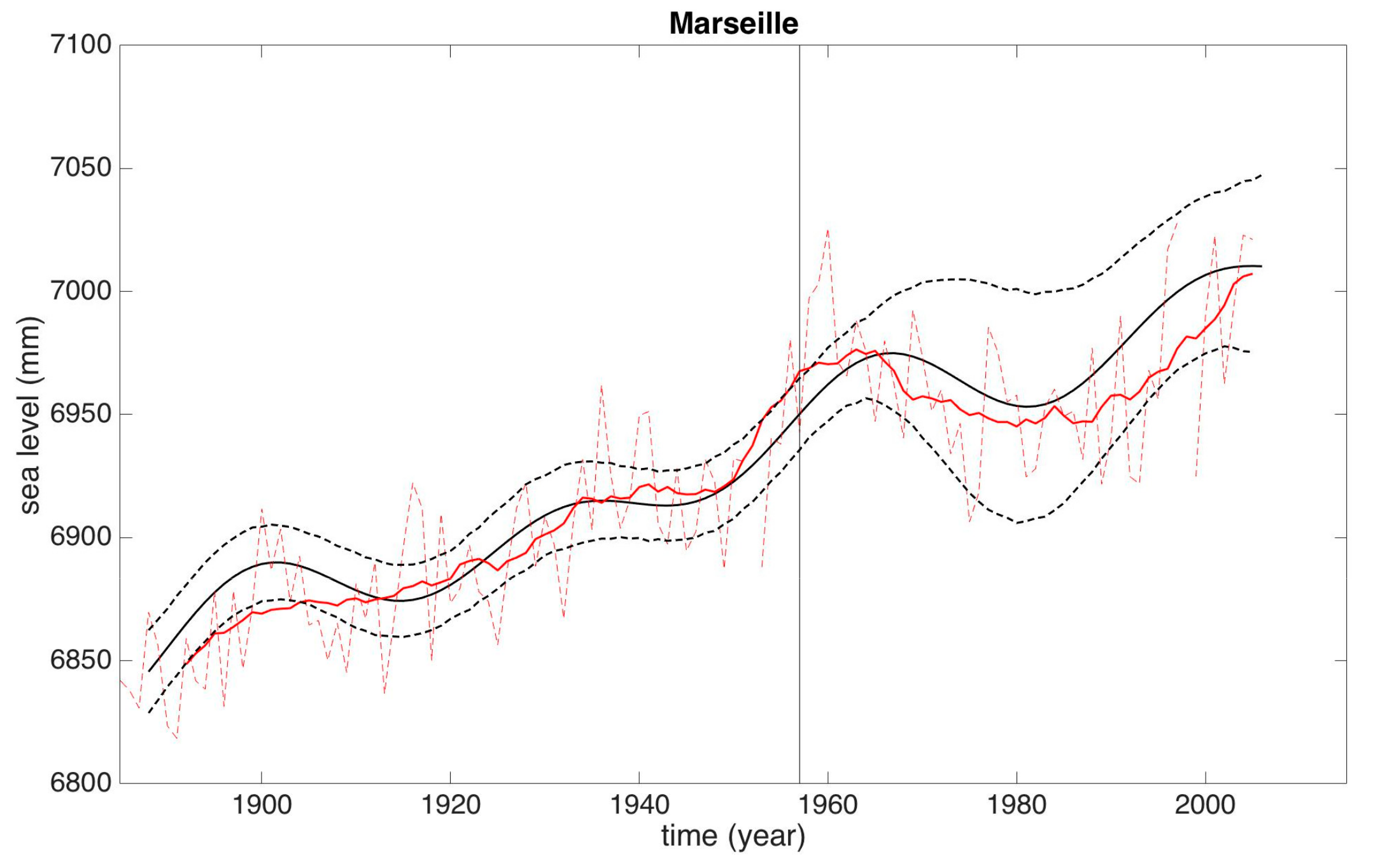
  • The normalized mean squared error (NMSE) between the 15 years smoothed and the model curves, after 1957, is 4.4 × 10⁻⁶ (if a model has a very low NMSE then it reproduces the data well);
  • The maximum and minimum discrepancy between the 15 years smoothed data and the model-derived sea levels are found in 1965 and 1997, respectively. Sea-level values are 6976 and 6977 mm for smoothed data, 6974 (6956, 6992) and 7000 (6968, 7032) mm for model data (values in parentheses represents the upper/lower 90% confidence interval).
The test shows that the modeling of the last 50 years of sea levels, based on the previous 70 years of data, fits the real sea levels within a 90% confidence interval well, thus indicating that the approach used is reliable.
To get sea-level projections at future times, time dependent rates from regional IPCC AR5 sea-level projections (spatial resolution: 1° × 1°), discussed in the Fifth Assessment Report of the IPCC-AR5 [73,74], and available from the Integrated Climate data Center-ICDC of the University of Hamburg (http://icdc.cen.uni-hamburg.de/1/daten/ocean/ar5-slr.html), were considered. Rates obtained under the Representative Concentration Pathways RCP2.6 and RCP8.5, providing the least and most amounts of future sea level rise respectively, were used. These data consist of mean values and upper/lower 90% confidence bounds obtained by summing up the contributions of several geophysical sources [73,74]: the thermosteric/dynamic contribution, from 21 CMIP5 coupled atmosphere-ocean general circulation models (AOGCMs); the surface mass balance and dynamic ice sheet contributions from Greenland and Antarctica; the glacier and land water storage contributions; the GIA and the inverse barometer effect. For each tide gauge record the IPCC regional sea-level rate was evaluated at the grid point closest to the location of the corresponding station. To take into account the VLM, we substituted the modeled GIA contribution to the IPCC rate with the measured cGPS rate that includes both real GIA and tectonics/anthropic vertical motion. When more than one cGPS station was present, the average VLM value was used (see Table 3). The IPCC rate, corrected for the measured VLM, represents the function r in Equation (4). Uncertainties for the sea-level estimations were then calculated by combining lower and upper sea level bounds from IPCC projection, errors from GPS measurements, and uncertainties from the model. Note that for the Bakar and Rovinj sea levels we used the modeled GIA component calculated from the mean of the ICE-5G model [75] and the Australian National University’s (ANU) ice sheet model [76] and subsequent improvements, since the measured VLM is not reliable.
Computed sea levels for the two considered IPCC scenarios are shown in Figure 7 and values at 2050 and 2100 (with respect to 2005) are indicated in Table 4. Let us first discuss the results without considering Venice P.S. A mean sea-level rise of 198 ± 102 mm by 2050 and 570 ± 255 mm by 2100 in the most severe RCP8.5 scenario, and 174 ± 97 mm and 342 ± 211 mm by 2050 and 2100, respectively, for the RCP2.6 scenario results from our modelling. In the most favorable scenario (RCP2.6) a sea-level rise between 142 ± 82 (Trieste) and 191 ± 106 (Split M.) mm by 2050, and between 259 ± 165 (Bakar) and 445 ± 200 (Dubrovnik) mm by 2100 is expected.
The most severe scenario projections indicate a sea-level rise between 150 ± 86 (Trieste) and 246 ± 95 (Dubrovnik) mm by 2050 and between 475 ± 203 (Bakar) and 681 ± 246 (Dubrovnik) mm by 2100. The combined effect of the VLM and SLNV produces an average increase of the sea level, with respect to pure IPCC projections, of 23/58 mm in RCP2.6 scenario and 37/65 mm in RCP8.5 scenario for 2050/2100 corresponding to a variation of about the 20% (2050) and 13% (2100). The maximum sea-level variation, with respect to pure IPCC projections, of 146/205 mm in RCP2.6 and 150/222 mm in RCP2.6 for 2050/2100 is found at Dubrovnik where the highest VLM rate is measured. The natural variability produces an average variation on the estimated sea level of about 20 (2050) and 10 (2100) mm with maximum values reaching about 65 mm with respect to the IPCC projections. Its average contribution, for the analyzed stations, is about the 9% in 2050 and 2.5% in 2100 (note that the SLNV contribution, in percentage, decreases when the effects of global changes and VLM increase). We remark that, although the contribution of the natural variability in the analyzed stations is of the order of few centimeters, its contribution is not negligible especially for coastlines that are more prone to marine flooding. In these areas, indeed, changes of some centimeters in projected sea levels can change the flooding scenarios [33].
The sea level at Venice deserves a separate discussion. At Venice P.S., future sea levels are strongly driven by the land subsidence that accounts alone up to 68% (2050) and 60% (2100) of the sea-level rise. VLM, together with the natural variability, accounts for up to 78% (2050) and 64% (2100) of the level rise. In the RCP2.6/RCP8.5 scenarios, the expected sea levels are 283 ± 103 mm/311 ± 114 mm (2050) and 603 ± 217 mm/818 ± 258 mm (2100) well above the values found for the other analyzed records. These values exceed, by about 220 (2050) and 385 mm (2100), the values obtained for Venice when pure IPCC scenarios are considered. These results have considerable implications for the area of the Venice lagoon, characterized by high-density of population, valuable historical setting, residential and industrial infrastructures, besides areas for agricultural use and national parks, for which sea-level rise can become a serious hazard.
The sea-level projections obtained in this study were finally compared with previous investigations in the same geographical areas. References [15,32] estimated the sea-level rise in the Venice area by making use of IPCC predictions, GIA modeling, and including the VLM contribution from geological and archeological data. By using the global IPCC 2007, in [15] the authors found a sea-level rise in 2100 (relative to the sea level average 1986–2005) of about 315 mm; an average sea level between 580 (minimum) and 996 mm (maximum) was estimated by [32], using the global IPCC AR5 RCP8.5 scenario. By modeling and combining the contributions of terrestrial ice melt, GIA and steric sea-level components, in [26] the authors elaborated a minimum and maximum sea-level rise scenario for sea level in 2050: sea levels at Marseille, Venice P.S., Trieste, Bakar were 60, 113, 113, 113 mm and 221, 227, 227, 229 mm respectively. Reference [14] presented a worldwide set of local sea-level projections up to 2100 and 2200 by modeling the contribution to the sea level through three ice sheet components, glacier and ice cap, oceanographic processes, and land water storage. A long-term, local, non-climatic sea-level change calculated through a Gaussian process model, based on historical tide gauge data, was also included to estimate the non-climatic contribution. A quite different approach consists of using a dynamical system model with spatial analysis capability [77,78,79] to assess the spatial variability of both temperature and sea-level changes over the 21st century. In this framework, temperature and sea level are considered as coupled variables whose behavior is described by two ordinary differential equations. After calibration through historical data, the model is able to provide reliable predictions of the two variables for the next century. For the Mediterranean Sea region, in particular, an average sea-level rise below 600 mm, relative to 1990, is expected.
The sea-level value from [15] (315 mm) is significantly lower than our RCP2.6 result for 2100 (603 ± 217 mm). This can be ascribed to the use of a global not upgraded IPCC model and an estimation of the VLM from geological and archeological data instead of GPS measurements. On the other hand, our RPC 8.5 results for 2100 are in agreement, within the error limits, with the results by [32]. Additionally, in this case small differences can arise from the use of a global IPCC model (instead of a local one) and the VLM estimation from geological data. Concerning the analysis proposed by [26], sea levels from their maximum scenario are in agreement with our predictions for both RCP2.6 and 8.5. Differences (mainly with their minimum scenario) possibly arise from differences in modeling ice melt, GIA, and steric components with respect to IPCC projections and from the lack of inclusion of the VLM contribution in their study.
Our results are in agreement with the mean sea-level values of [14], within the uncertainty limit, for both 2050 and 2100 at the nine analyzed locations. Differences between the two results are smaller (at most 10%) for the records spanning a longer period (Marseille, Trieste, and Genova) which indicates that both analyses seem to converge when longer time series are considered. We recall that both the approaches use observationally based rates to account for local effects in the sea-level predictions and both the EMD as well as the statistical approach from [14] are more accurate when longer data points are available. Small differences can also be due to differences in modeling ice sheet components, glacier and ice cap, oceanographic processes, and land water storage with respect to IPCC projections. Regarding the results from the Venice station, differences reaching 27% were found. Due to the strong subsidence affecting only the Venice area, and not the entire North Adriatic Sea, we believe that an approach that takes into account the punctual vertical land motion measured closer to the tide gauge station is more suitable for modeling this effect on the sea-level. A comparison of the sea level in 2100 in the Mediterranean Sea area from [77] shows very good agreement with our results when the RCP85 scenario is considered. Indeed, when averaged over all stations (excluding Venice) and reported to the same time basis (year 1990) as [77] we found an average sea-level of 626 ± 255 mm that fits well, within the uncertainty limits, the value found by [77].
Finally, the modeling of the effect of the natural variability on future sea-level projections, present in this study, can also introduce, to a lesser extent, differences with sea-level estimations from the works mentioned above.

5. Conclusions

Sea levels for 2050 and 2100 at nine locations in the Central-Northern Mediterranean coasts were estimated from tide gauge data by including the contribution of both the vertical land motion and the natural variability. The VLM was inferred at a set of locations nearby tide gauges through continuous GPS measurements. The SLNV was estimated by the EMD analysis on the tide gauge data. The EMD approach revealed modes at characteristic time scales in the ranges 20–30 and >45 years, associated with the long-term natural variability, resulting from the combined effect of teleconnection patterns. Expected sea levels in 2050 and 2100 were then estimated by using IPCC projection, for the time dependent sea-level rate, the measured VLM rate, and a superposition of periodic functions, whose properties were obtained from the EMD results, to model the contribution of the long-term variability. Results (excluding the Venice P.S. tide gauge station) provided a mean sea-level rise of 198 ± 102 mm by 2050 and 570 ± 255 mm by 2100 in the most severe RCP8.5 scenario, while a lower bound is estimated to be 174 ± 97 and 342 ± 211 mm by 2050 and 2100, respectively, for the RCP2.6 scenario. The contribution of natural variability to local sea-level variations is significant and can reach, on average, up to the 9% with respect to the sea-level changes induced only by global climate change. VLM and SLNV together account, on average, for about the 15% of the sea-level variation.
In the Venice lagoon, the land subsidence is increasing the local sea-level rise. By taking into account VLM rates measured by the cGPS stations in this area, relative sea levels are expected to reach 603 ± 217 and 818 ± 258 mm in 2100 for the RCP2.6 and RCP8.5 scenarios, respectively. In particular, at the Venice P.S. tidal station, VLM and SLNV contribute more than the 60% to the expected sea-level rise.
Finally, our analysis shows that the contribution of local effects, such as the natural variability and the vertical land motion, play a key role in local sea-level rise projections. Effects are even more relevant for low elevated coastal areas where marine ingression may represent a potential hazard for the environment and human activities. Even in the more optimistic scenario, the estimated sea-level rise will have an important impact along the coasts, causing diffuse erosion of the shorelines, hence determining serious impacts on many coastal areas, increasing the hazard related to flooding events, storm surges, and possibly tsunamis. In subsiding areas, like the Venice Lagoon, severe environmental impact with subsequent loss of economic value of shores and coastal infrastructures can be reasonably expected before 2100. In this regard, land planners and decision makers should take into account the rising sea levels reported in this study for cognizant coastal management.

Author Contributions

Conceptualization, A.V. and M.A.; Formal analysis, A.V. and E.S.; Funding acquisition, M.A.; Methodology, A.V.; Project administration, M.A.; Supervision, M.A. and F.F.; Validation, A.V.; Writing – original draft, A.V.; Writing—review & editing, M.A., E.S. and F.F.

Funding

This work was carried out under the umbrella of the SAVEMEDCOASTS project “Sea level rise scenarios along the Mediterranean coasts”, funded by the EU (www.savemedcoasts.eu; agreement number ECHO/SUB/2016/742473/PREV16).

Acknowledgments

We acknowledge two anonymous reviewers for the useful comments.

Conflicts of Interest

The authors declare no conflict of interest.

References

  1. Vermeer, M.; Rahmstorf, S. Global sea level linked to global temperature. Proc. Natl. Acad. Sci. USA 2009, 106, 21527–21532. [Google Scholar] [CrossRef] [PubMed] [Green Version]
  2. Church, J.A.; White, N.J. Sea-Level Rise from the Late 19th to the Early 21st Century. Surv. Geophys. 2011, 32, 585–602. [Google Scholar] [CrossRef] [Green Version]
  3. Kemp, A.C.; Horton, B.P.; Donnelly, J.P.; Mann, M.E.; Vermeer, M.; Rahmstorf, S. Climate related sea-level variations over the past two millennia. Proc. Natl. Acad. Sci. USA 2011, 108, 11017–11022. [Google Scholar] [CrossRef] [PubMed] [Green Version]
  4. Lambeck, K.; Woodroffe, C.D.; Antonioli, F.; Anzidei, M.; Gehrels, W.R.; Laborel, J.; Wright, A.J. Paleoenvironmental Records, Geophysical Modeling, and Reconstruction of Sea-Level Trends and Variability on Centennial and Longer Timescales. In Understanding Sea-Level Rise and Variability; Blackwell: Hoboken, NJ, USA, 2010; pp. 61–121. [Google Scholar]
  5. Meyssignac, B.; Cazenave, A. Sea level: A review of present-day and recent-past changes and variability. J. Geodyn. 2012, 58, 96–109. [Google Scholar] [CrossRef]
  6. Mitchum, G.T.; Nerem, R.S.; Merrifield, M.A.; Gehrels, W.R. Modern sea level changes estimates. In Understanding Sea Level Rise and Variability; Church, J.A., Woodworth, P.L., Aarup, T., Wilson, W.S., Eds.; Wiley-Blackwell Publishing: London, UK, 2010. [Google Scholar]
  7. Jevrejeva, S.; Moore, J.; Grinsted, A. Sea level projections to AD2500 with a new generation of climate change scenarios. Glob. Planet. Chang. 2012, 80, 14–20. [Google Scholar] [CrossRef]
  8. Wöppelmann, G.; Marcos, M. Coastal sea level rise in southern Europe and the nonclimate contribution of vertical land motion. J. Geophys. Res. Space Phys. 2012, 117. [Google Scholar] [CrossRef] [Green Version]
  9. Anzidei, M.; Lambeck, K.; Antonioli, F.; Furlani, S.; Mastronuzzi, G.; Serpelloni, E.; Vannucci, G. Coastal structure, sea-level changes and vertical motion of the land in the Mediterranean. Geol. Soc. Lond. Spéc. Publ. 2014, 388, 453–479. [Google Scholar] [CrossRef]
  10. Tsimplis, M.N.; Calafat, F.M.; Marcos, M.; Jorda, G.; Gomis, D.; Fenoglio-Marc, L.; Struglia, M.V.; Josey, S.A.; Chambers, D.; Fenoglio-Marc, L. The effect of the NAO on sea level and on mass changes in the Mediterranean Sea. J. Geophys. Res. Oceans 2013, 118, 944–952. [Google Scholar] [CrossRef] [Green Version]
  11. Fenoglio-Marc, L.; Rietbroek, R.; Grayek, S.; Becker, M.; Kusche, J.; Stanev, E. Water mass variation in the Mediterranean and Black Seas. J. Geodyn. 2012, 59, 168–182. [Google Scholar] [CrossRef]
  12. Fenoglio-Marc, L.; Mariotti, A.; Sannino, G.; Meyssignac, B.; Carillo, A.; Struglia, M.; Rixen, M. Decadal variability of net water flux at the Mediterranean Sea Gibraltar Strait. Glob. Planet. Chang. 2013, 100, 1–10. [Google Scholar] [CrossRef] [Green Version]
  13. Lambeck, K.; Purcell, A. Sea-level change in the Mediterranean Sea since the LGM: Model predictions for tectonically stable areas. Quat. Sci. Rev. 2005, 24, 1969–1988. [Google Scholar] [CrossRef]
  14. Kopp, R.E.; Horton, R.M.; Little, C.M.; Mitrovica, J.X.; Oppenheimer, M.; Rasmussen, D.J.; Strauss, B.H.; Tebaldi, C. Probabilistic 21st and 22nd century sea-level projections at a global network of tide-gauge sites. Earth’s Future 2014, 2, 383–406. [Google Scholar] [CrossRef]
  15. Lambeck, K.; Antonioli, F.; Anzidei, M.; Ferranti, L.; Leoni, G.; Scicchitano, G.; Silenzi, S. Sea level change along the Italian coast during the Holocene and projections for the future. Quat. Int. 2011, 232, 250–257. [Google Scholar] [CrossRef]
  16. Douglas, B.C. Global sea rise: A redetermination. Surv. Geophys. 1997, 18, 270–292. [Google Scholar] [CrossRef]
  17. Knutti, R.; Stocker, T.F. Influence of the Thermohaline Circulation on Projected Sea Level Rise. J. Clim. 2000, 13, 1997–2001. [Google Scholar] [CrossRef]
  18. Rahmstorf, S. A Semi-Empirical Approach to Projecting Future Sea-Level Rise. Science 2007, 315, 368–370. [Google Scholar] [CrossRef] [PubMed] [Green Version]
  19. Rahmstorf, S.; Cazenave, A.; Church, J.A.; Hansen, J.E.; Keeling, R.F.; Parker, D.E.; Somerville, R.C.J. Recent Climate Observations Compared to Projections. Science 2007, 316, 709. [Google Scholar] [CrossRef] [PubMed]
  20. Milne, G.A.; Gehrels, W.R.; Hughes, C.W.; Tamisiea, M.E. Identifying the causes of sea-level change. Nat. Geosci. 2009, 2, 471–478. [Google Scholar] [CrossRef] [Green Version]
  21. Tsimplis, M.; Marcos, M.; Colin, J.; Somot, S.; Pascual, A.; Shaw, A. Sea level variability in the Mediterranean Sea during the 1990s on the basis of two 2d and one 3d model. J. Mar. Syst. 2009, 78, 109–123. [Google Scholar] [CrossRef]
  22. Tsimplis, M.; Spada, G.; Marcos, M.; Flemming, N. Multi-decadal sea level trends and land movements in the Mediterranean Sea with estimates of factors perturbing tide gauge data and cumulative uncertainties. Glob. Planet. Chang. 2011, 76, 63–76. [Google Scholar] [CrossRef]
  23. Church, J.A.; Aarup, T.; Woodworth, P.L.; Wilson, W.S.; Nicholls, R.J.; Rayner, R.; Lambeck, K.; Mitchum, G.T.; Steffen, K.; Cazenave, A.; et al. Sea-Level Rise and Variability: Synthesis and Outlook for the Future. In Understanding Sea-Level Rise and Variability, 1st ed.; Church, A.J., Woodworth, P.L., Aarup, T., Wilson, S., Eds.; Blackwell Publishing Ltd.: Hoboken, NJ, USA, 2010. [Google Scholar]
  24. Cazenave, A.; Remy, F. Sea level and climate: Measurements and causes of changes. Wiley Interdiscip. Rev. Clim. Chang. 2011, 2, 647–662. [Google Scholar] [CrossRef]
  25. Zhang, X.; Church, J.A. Sea level trends, interannual and decadal variability in the Pacific Ocean. Geophys. Res. Lett. 2012, 39, 21701. [Google Scholar] [CrossRef]
  26. Galassi, G.; Spada, G. Sea-level rise in the Mediterranean Sea by 2050: Roles of terrestrial ice melt, steric effects and glacial isostatic adjustment. Glob. Planet. Chang. 2014, 123, 55–66. [Google Scholar] [CrossRef]
  27. Han, W.; Stammer, D.; Meehl, G.A.; Hu, A.; Sienz, F.; Zhang, L. Multi-Decadal Trend and Decadal Variability of the Regional Sea Level over the Indian Ocean since the 1960s: Roles of Climate Modes and External Forcing. Climate 2018, 6, 51. [Google Scholar] [CrossRef]
  28. Brambati, A.; Carbognin, L.; Quaia, T.; Teatini, P.; Tosi, L. The Lagoon of Venice: Geological setting, evolution and land subsidence. Episodes 2003, 26, 264–268. [Google Scholar]
  29. Carbognin, L.; Teatini, P.; Tosi, L. Eustacy and land subsidence in the Venice Lagoon at the beginning of the new millennium. J. Mar. Syst. 2004, 51, 345–353. [Google Scholar] [CrossRef]
  30. De Conto, R.M.; Pollard, D. Contribution of Antarctica to past and future sea-level rise. Nature 2016, 531, 591–597. [Google Scholar] [CrossRef]
  31. Syvitski, J.P.M.; Kettner, A.J.; Overeem, I.; Hutton, E.W.H.; Hannon, M.T.; Brakenridge, G.R.; Day, J.; Vörösmarty, C.; Saito, Y.; Giosan, L.; et al. Sinking deltas due to human activities. Nat. Geosci. 2009, 2, 681–686. [Google Scholar] [CrossRef]
  32. Antonioli, F.; Anzidei, M.; Amorosi, A.; Presti, V.L.; Mastronuzzi, G.; Deiana, G.; De Falco, G.; Fontana, A.; Fontolan, G.; Lisco, S.; et al. Sea-level rise and potential drowning of the Italian coastal plains: Flooding risk scenarios for 2100. Quat. Sci. Rev. 2017, 158, 29–43. [Google Scholar] [CrossRef] [Green Version]
  33. Bosman, A.; Carluccio, R.; Casalbore, D.; Caracciolo, F.D.; Esposito, A.; Nicolosi, I.; Pietrantonio, G.; Vecchio, A.; Carmisciano, C.; Chiappini, M.; et al. Flooding scenarios due to land subsidence and sea-level rise: A case study for Lipari Island (Italy). Terra Nova 2017, 29, 44–51. [Google Scholar]
  34. Marsico, A.; Lisco, S.; Presti, V.L.; Antonioli, F.; Amorosi, A.; Anzidei, M.; Deiana, G.; De Falco, G.; Fontana, A.; Fontolan, G.; et al. Flooding scenario for four Italian coastal plains using three relative sea level rise models. J. Maps 2017, 13, 961–967. [Google Scholar] [CrossRef] [Green Version]
  35. Douglas, B.C. Global sea level rise. J. Geophys. Res. 1991, 96, 6981–6992. [Google Scholar] [CrossRef] [Green Version]
  36. Douglas, B.C. Global sea level rise acceleration. J. Geophys. Res. 1992, 97, 12699–12796. [Google Scholar] [CrossRef]
  37. Visser, H.; Dangendorf, S.; Petersen, A.C. A review of trend models applied to sea level data with reference to the “acceleration-deceleration debate”. J. Geophys. Res. Oceans 2015, 120, 3873–3895. [Google Scholar] [CrossRef]
  38. Huang, N.E.; Shen, Z.; Long, S.R.; Wu, M.C.; Shih, E.H.; Zheng, Q.; Tung, C.C.; Liu, H.H. The empirical mode decomposition and the Hilbert spectrum for non-stationary time series analysis. Proc. R. Soc. Lond. 1998, 454, 903–995. [Google Scholar] [CrossRef]
  39. Vecchio, A.; Capparelli, V.; Carbone, V. The complex dynamics of the seasonal component of USA’s surface temperature. Atmos. Chem. Phys. 2010, 10, 9657–9665. [Google Scholar] [CrossRef]
  40. Vecchio, A.; Anzidei, M.; Capparelli, V.; Carbone, V.; Guerra, I. Has the Mediterranean Sea felt the March 11th, 2011, Mw 9.0 Tohoku-Oki earthquake? Europhys. Lett. 2012, 98, 59001. [Google Scholar] [CrossRef]
  41. Vecchio, A.; Anzidei, M.; Carbone, V. New insights on the tsunami recording of the May, 21, 2003, Mw 6.9 Boumerdès earthquake from tidal data analysis. J. Geodyn. 2014, 79, 39–49. [Google Scholar] [CrossRef]
  42. Breaker, L.C.; Ruzmaikin, A. The 154-year record of sea level at San Francisco: Extracting the long-term trend, recent changes, and other tidbits. Clim. Dyn. 2011, 36, 545–559. [Google Scholar] [CrossRef]
  43. Ezer, T.; Corlett, W.B. Is sea level rise accelerating in the Chesapeake Bay? A demonstration of a novel new approach for analyzing sea level data. Geophys. Res. Lett. 2012, 39, L19605. [Google Scholar] [CrossRef]
  44. Ezer, T.; Atkinson, L.P.; Corlett, W.B.; Blanco, J.L. Gulf Stream’s induced sea level rise and variability along the U.S. mid-Atlantic coast. J. Geophys. Res. Ocean 2013, 118, 685–697. [Google Scholar] [CrossRef]
  45. Chambers, D.P. Evaluation of empirical mode decomposition for quantifying multi-decadal variations and acceleration in sea level records. Nonlinear Proc. Geophys. 2015, 22, 157–166. [Google Scholar] [CrossRef] [Green Version]
  46. Wu, Z.; Huang, N.E. A study of the characteristics of white noise using the empirical mode decomposition method. Proc. R. Soc. Lond. A 2004, 460, 1597–1611. [Google Scholar] [CrossRef]
  47. Frankcombe, L.M.; Von der Heydt, A.; Dijkstra, H.A. North Atlantic multidecadal climate variability: An Investigation of dominant time scales and processes. J. Climatol. 2010, 23, 3626–3638. [Google Scholar] [CrossRef]
  48. Marshall, J.; Johnson, H.; Goodman, J. A study of the interaction of the North Atlantic Oscillation with the ocean circulation. J. Clim. 2001, 14, 1399–1421. [Google Scholar] [CrossRef]
  49. Bellucci, A.; Gualdi, S.; Scoccimarro, E.; Navarra, A. NAO-ocean circulation interactions in a coupled general circulation model. Clim. Dyn. 2008, 31, 759–777. [Google Scholar] [CrossRef]
  50. Fan, M.; Schneider, E.K. Observed decadal North Atlantic tripole SST variability. Part I: Weather noise forcing and coupled response. J. Atmos. Sci. 2012, 69, 35–50. [Google Scholar]
  51. Knudsen, M.F.; Seidenkrantz, M.-S.; Jacobsen, B.H.; Kuijpers, A. Tracking the Atlantic Multidecadal Oscillation through the last 8,000 years. Nat. Commun. 2011, 2, 178. [Google Scholar] [CrossRef]
  52. Hubeny, J.B.; King, J.W.; Santos, A. Subdecadal to multidecadal cycles of Late Holocene North Atlantic climate variability preserved by estuarine fossil pigments. Geology 2006, 34, 569–572. [Google Scholar] [CrossRef] [Green Version]
  53. Calafat, F.M.; Jordà, G.; Marcos, M.; Gomis, D. Comparison of Mediterranean sea level variability as given by three baroclinic models. J. Geophys. Res. 2012, 117, c02009. [Google Scholar] [CrossRef]
  54. Calafat, F.M.; Chambers, D.P.; Tsimplis, M.N. Mechanisms of decadal sea level variability in the eastern North Atlantic and the Mediterranean Sea. J. Geophys. Res. 2012, 117, c09022. [Google Scholar] [CrossRef]
  55. Tsimplis, M.N.; Shaw, A.G.P. The forcing of mean sea level variability around Europe. Glob. Planet. Chang. 2008, 63, 196–202. [Google Scholar] [CrossRef]
  56. Kosaka, Y.; Xie, S.-P. Recent global-warming hiatus tied to equatorial Pacific surface cooling. Nature 2013, 501, 403–407. [Google Scholar] [CrossRef] [PubMed] [Green Version]
  57. Zhang, L. The roles of external forcing and natural variability in global warming hiatuses. Clim. Dyn. 2016, 47, 3157–3169. [Google Scholar] [CrossRef]
  58. Kosaka, Y.; Xie, S.-P. The tropical Pacific as a key pacemaker of the variable rates of global warming. Nat. Geosci. 2016, 9, 669–673. [Google Scholar] [CrossRef]
  59. Marullo, S.; Artale, V.; Santoleri, R. The SST Multidecadal Variability in the Atlantic–Mediterranean Region and Its Relation to AMO. J. Clim. 2011, 24, 4385–4401. [Google Scholar] [CrossRef]
  60. Vigo, M.; Sánchez-Reales, J.; Trottini, M.; Chao, B. Mediterranean Sea level variations: Analysis of the satellite altimetric data, 1992–2008. J. Geodyn. 2011, 52, 271–278. [Google Scholar] [CrossRef]
  61. Devoti, R.; D’Agostino, N.; Serpelloni, E.; Pietrantonio, G.; Riguzzi, F.; Avallone, A.; Cavaliere, A.; Cheloni, D.; Cecere, G.; D’Ambrosio, C.; et al. The mediterranean crustal motion map compiled at INGV. Ann. Geophys. 2017, 60. [Google Scholar] [CrossRef]
  62. Serpelloni, E.; Faccenna, C.; Spada, G.; Dong, D.; Williams, S.D.P. Vertical GPS ground motion rates in the Euro-Mediterranean region: New evidence of velocity gradients at different spatial scales along the Nubia-Eurasia plate boundary. J. Geophys. Res. Solid Earth 2013, 118, 6003–6024. [Google Scholar] [CrossRef] [Green Version]
  63. Altamimi, Z.; Collilieux, X.; Métivier, L. ITRF2008: An improved solution of the international terrestrial reference frame. J. Geod. 2011, 85, 457–473. [Google Scholar] [CrossRef]
  64. Antonioli, F.; Anzidei, M.; Lambeck, K.; Auriemma, R.; Gaddi, D.; Furlani, S.; Orrù, P.; Solinas, E.; Gaspari, A.; Karinja, S.; et al. Sea level change during Holocene from Sardinia and northeastern Adriatic (Central Mediterranean sea) from archaeological and geomorphological data. Quat. Sci. Rev. 2007, 26, 2463–2524. [Google Scholar] [CrossRef]
  65. Carbognin, L.; Gatto, P.; Mozzi, G.; Gambolati, G.; Ricceri, G. New trend in the subsidence of Venice. In Proceedings of the Anaheim Symposium, Anaheim, CA, USA, 13–17 December 1976. [Google Scholar]
  66. Guidoboni, E.; Comastri, A. Catalogue of Earthquakes and Tsunami in the Mediterranean Area from the 11th to the 15th Century; INGV-SGA: Rome, Italy, 2007. [Google Scholar]
  67. Carbognin, L.; Teatini, P.; Tomasin, A.; Tosi, L. Global change and relative sea level rise at Venice: What impact in term of flooding. Clim. Dyn. 2010, 35, 1039–1047. [Google Scholar] [CrossRef]
  68. Lyu, K.; Zhang, X.; Church, J.A.; Slangen, A.B.A.; Hu, J. Time of emergence for regional sea-level change. Nat. Clim. Chang. 2014, 4, 1006–1010. [Google Scholar] [CrossRef]
  69. Bordbar, M.H.; Martin, T.; Latif, M.; Park, W. Effects of long-term variability on projections of twenty-first century dynamic sea level. Nat. Clim. Chang. 2015, 5, 343–347. [Google Scholar] [CrossRef]
  70. Carson, M.; Köhl, A.; Stammer, D. The Impact of Regional Multidecadal and Century-Scale Internal Climate Variability on Sea Level Trends in CMIP5 Models. J. Clim. 2015, 28, 853–861. [Google Scholar] [CrossRef]
  71. Kopp, R.E.; Hay, C.C.; Little, C.M.; Mitrovica, J.X. Geographic Variability of Sea-Level Change. Curr. Clim. Chang. Rep. 2015, 1, 192–204. [Google Scholar] [CrossRef] [Green Version]
  72. Little, C.M.; Horton, R.M.; Kopp, R.; Oppenheimer, M.; Yip, S. Uncertainty in Twenty-First-Century CMIP5 Sea Level Projections. J. Clim. 2015, 28, 838–852. [Google Scholar] [CrossRef]
  73. Church, J.A.; Clark, P.U.; Cazenave, A.; Gregory, J.; Jevrejeva, S.; Levermann, A.; Merrifield, M.; Milne, G.; Nerem, R.S.; Nunn, P.; et al. Sea level change. In Climate Change 2013: The Physical Science Basis; Stocker, T.F., Qin, D.G.-K., Plattner, M., Tignor, S.K., Allen, J., Boschung, A., Nauels, Y., Bex, X.V., Midgley, P.M., Eds.; Cambridge University Press: Cambridge, UK; New York, NY, USA, 2013. [Google Scholar]
  74. Church, J.A.; Clark, P.U.; Cazenave, A.; Gregory, J.; Jevrejeva, S.; Levermann, A.; Merrifield, M.; Milne, G.; Nerem, R.S.; Nunn, P.; et al. Sea Level Change Supplementary Material. In Climate Change 2013: The Physical Science Basis; Contribution of Working Group I to the Fifth Assessment Report of the Intergovernmental Panel on Climate Change; Stocker, T.F., Qin, D.G.-K., Plattner, M., Tignor, S.K., Allen, J., Boschung, A., Nauels, Y., Bex, X.V., Midgley, P.M., Eds.; Cambridge University Press: Cambridge, UK; New York, NY, USA, 2013. [Google Scholar]
  75. Peltier, W.R. Global glacial isostasy and the surface of the ice-age earth: The ICE-5G (VM2) model and GRACE. Annu. Rev. Earth Planet. Sci. 2004, 32, 111–149. [Google Scholar] [CrossRef]
  76. Lambeck, K.; Smither, C.; Johnston, P. Sea-level change, glacial rebound and mantle viscosity for northern Europe. Geophys. J. Int. 1998, 134, 102–144. [Google Scholar] [CrossRef]
  77. Aral, M.M.; Chang, B. Spatial Variation of Sea Level Rise at Atlantic and Mediterranean Coastline of Europe. Water 2017, 9, 522. [Google Scholar] [CrossRef]
  78. Chang, B.; Guan, J.; Aral, M.M. A Scientific Discourse: Climate Change and Sea-Level Rise. ASCE J. Hydrol. Eng. 2015, 20, A4014003. [Google Scholar] [CrossRef]
  79. Chang, B.; Guan, J.; Aral, M.M. Modeling Spatial Variations of Sea Level Rise and Corresponding Inundation Impacts: A Case Study for Florida, USA. Water Qual. Expo. Health 2013, 6, 39–51. [Google Scholar] [CrossRef]
Figure 1. Location of the nine analyzed tidal stations: Marseille (5.35°–43.32°, 1885–2012), Trieste (13.76°–45.57°, 1875–2012), Genova (9.92°–44.41°, 1884–1997), Venice Punta Salute (12.32°–45.39°, 1909–2000), Bakar (14.5°–45.30°, 1930–2011), Dubrovnik (19.13°–42.65°, 1956−2009), Rovinj (13.64°–45.06°, 1955–2011), Split RT Marjana (16.39°–43.51°, 1952–2011), Split Gradska Luka (16.44°–43.51°, 1954–2011). Coordinates of the station and time span of recordings are indicated in parentheses.
Water 11 01480 g001
Figure 2. Time series of the monthly mean tidal records from stations in Figure 1 (data from www.psmsl.org). Red lines show linear regressions on the data (see the text for details).
Water 11 01480 g002
Figure 3. Function LLT(t) (black line), obtained by summing up IMFs at timescales >15 years and the residue, and the best-fit function LM(t) (red line) described by Equation (4).
Water 11 01480 g003
Figure 4. EMD reconstruction by using IMFs with timescale >15 years (the residue rn(t) has not been added up) for the four closest stations in the North Adriatic Sea.
Water 11 01480 g004
Figure 5. Map of the absolute (i.e., IGb08 frame) vertical velocities for the continuous GPS (cGPS) stations used in this work. Black dots refer to the stations ROGS (Bakar) and RIGS (Rovinj) for which, due to the limited available data, calculated vertical land motion (VLM) are not reliable.
Water 11 01480 g005
Figure 6. Sea levels in the period 1888–2007 at Marseille as estimated by deriving the model from the first 70 years (1888–1957) of tidal data. Fit parameters are: r = 1.57 ± 0.04; c = 3882 ± 75; A = 13.8 ± 1.0, 9.8 ± 1.01; Φ = 1.22 ± 0.06, 1.89 ± 0.09, R2 = 0.91. The model (black line) with 90% confidence interval (enclosed by black dashed lines), sea-level data at 1 year of resolution (red dashed line) and smoothed by a 15-year sliding window (red line), are shown. The vertical bar marks the boundary between sea level data used for the model (left) and estimated sea levels (right).
Water 11 01480 g006
Figure 7. Sea-level height up to 2100 for the analyzed stations, as obtained by the model of Equation (4) that includes VLM and AR5 RCP2.6 (blue line) and RCP8.5 (red line) rate. Color bands represent the 90% confidence interval, obtained by including uncertainties from the model, VLM, and AR5 trend. The black line represents sea levels when the constant trend obtained from fits is used. Since cGPS data are not reliable, the contribution of VLM is not included for Bakar and Rovinj.
Water 11 01480 g007
Table 1. Characteristic periods (years) of the significant intrinsic mode functions (IMFs) with a characteristic timescale >15 years, obtained by the Empirical Mode Decomposition (EMD) for the analyzed data set. Errors are estimated as the standard deviation.
Tide Gauge Stationnj = 7j = 8j = 9j = 10j = 11j = 12j = 13
Marseille15 29.8 ± 14.536.5 ± 7.443.1 ± 15.663.1 ± 21.2
Trieste 15 19.8 ± 4.427.0 ± 3.637.6 ± 8.852.2 ± 12.776.3 ± 45.9
Genova1015.3 ± 2.532.2 ± 2.1
Venice P.S.12 16.0 ± 2.521.0 ± 2.144.3 ± 5.0
Bakar12 16.9 ± 2.829.4 ± 7.758.0 ± 4.9
Dubrovnik11 17.0 ± 2.549.4 ± 19.2
Rovinj11 16.2 ± 5.636.6 ± 8.3
Split M.13 18.6 ± 3.421.7 ± 4.533.7 ± 25.9
Split G.1117.8 ± 3.749.6 ± 16.4
Table 2. Fit parameters and adjusted R-square values for the analyzed data set. Uncertainties define the 90% confidence limits.
Tide Gauge StationLinear Fit
(mm a−1)
r
(mm a−1)
c
(mm)
A
(mm)
ΦR2
Marseille1.22 ± 0.101.28 ± 0.014436 ± 1210.1 ± 0.34.03 ± 0.300.9948
11.1 ± 0.3−0.84 ± 0.03
16.1 ± 0.51.84 ± 0.04
18.7 ± 0.5−0.42 ± 1.54
Trieste1.22 ± 0.151.59 ± 0.053874 ± 8610.8 ± 0.42.54 ± 2.110.9844
13.2 ± 0.82.34 ± 0.05
10.3 ± 1.74.87 ± 0.73
19.1 ± 2.9−3.04 ± 0.13
21.9 ± 2.02.52 ± 0.05
Genova1.07 ± 0.241.20 ± 0.034618 ± 547.8 ± 0.7−1.93 ± 0.080.9254
12.1 ± 0.62.58 ± 0.24
Venice P.S.2.43 ± 0.232.78 ± 0.041615 ± 7413.1 ± 1.1−0.61 ± 0.090.9579
18.8 ± 1.3−2.03 ± 0.07
23.8 ± 1.32.10 ± 0.05
Bakar0.9 ± 0.370.88 ± 0.155323 ± 30621.1 ± 1.33.36 ± 0.890.9515
21.9 ± 2.2−1.63 ± 0.11
12.1 ± 0.7−0.66 ± 2.36
Dubrovnik0.90 ± 0.441.24 ± 0.054520 ± 10427.4 ± 0.62.41 ± 0.020.9662
20.6 ± 0.8−1.74 ± 0.04
Rovinj0.38 ± 0.430.97 ± 0.105144 ± 19026.5 ± 0.9−0.45 ± 0.030.9014
20.3 ± 1.21.76 ± 0.09
Split M.0.35 ± 0.380.17 ± 0.026671 ± 2918.8 ± 0.32.62 ± 0.020.9888
26.8 ± 0.4−1.84 ± 0.01
26.4 ± 0.41.35 ± 0.01
Split G. L.0.51 ± 0.401.87 ± 0.073360 ± 13717.1 ± 0.70.68 ± 0.040.9434
35.1 ± 0.11.48 ± 0.03
Table 3. VLM measured at the cGPS station closest to the tide gauges used in this work. The cGPS station name, position, rate of VLM, time interval of the time series, mean VLM, and the closest tide gauges to the cGPS stations are indicated. Negative sign in the VLM corresponds to land subsidence.
GNSS
Station
LonLatVLM
(mm a−1)
Time IntervalAverage VLM
(mm a−1)
Tide Gauge
Location
PRIE5.372743.2768−0.65 ± 0.552007.6397–2018.0890−0.61 ± 0.43Marseille
MARS5.353843.2788−0.58 ± 0.311998.5465–2018.0917
TRIE13.763545.7098−0.20 ± 0.362003.1054–2018.0917−0.08 ± 0.49Trieste
TRI113.787845.66060.04 ± 0.612007.7821–2016.8948
GENV8.880944.41520.74 ± 0.902008.4631–2014.7602−0.12 ± 1.54Genova
GENO8.921144.4194−0.25 ± 0.301998.5575–2018.0917
GENA8.948244.3976−0.51 ± 4.302016.6270–2017.9273
GENU8.959344.4027−0.50 ± 0.682009.9465–2017.9986
DUB218.110342.6502−1.13 ± 0.962011.9739–2018.0917−1.56 ± 0.72Dubrovnik
DUBR18.110442.6500−1.99 ± 0.482000.7226–2012.7363
SPLT16.438543.50660.56 ± 0.772005.0013–2012.25270.56 ± 0.77Split
CGIA12.265545.2065−2.91 ± 0.832010.9630–2018.0917−3.30 ± 0.85Venice
SFEL12.291345.2300−4.57 ± 0.672001.5465–2011.1657
VEAR12.357845.4379−2.17 ± 1.352006.1602–2010.7164
VEN112.354145.4306−1.46 ± 0.652009.8068–2018.0917
VENE12.332045.4370−0.89 ± 0.822001.0863–2007.5630
VE0112.333945.4375−2.22 ± 1.562007.8506–2011.1821
MSTR12.238645.4904−2.50 ± 0.792007.8890–2014.6315
TREP12.454745.4677−8.45 ± 1.692004.1871–2008.0724
CAVA12.582745.4794−2.71 ± 0.582001.5438–2011.1657
TGPO12.228345.0031−4.89 ± 0.532007.3164–2018.0917
PTO112.334144.9515−4.26 ± 0.592008.4631–2017.9301
GARI12.249444.6769−3.25 ± 0.662009.3958–2018.0917
RAVE12.191944.4053−4.23 ± 0.582008.0259–2017.9986
BEVA13.069445.6719−1.69 ± 0.572008.0368–2018.0917
Table 4. Sea levels for 2050 and 2100, with respect to 2005, at the tide gauge for the two scenarios RCP2.6 and RCP8.5 including both the VLM and sea level natural variability (SLNV) contribution. Uncertainties define the 90% confidence limits. Time span used for the modeling and duration of raw records (in parenthesis) are also indicated. Since cGPS data are not reliable, the contribution of VLM is not included for Bakar and Rovinj.
Tide Gauge Station
(Duration)
Sea Level
(mm)
RCP2.6
Sea Level
(mm)
RCP8.5
2050210020502100
Marseille182 ± 79364 ± 167208 ± 79602 ± 240
1888–2009
(128 years)
Trieste142 ± 82336 ± 197150 ± 86523 ± 237
1901–2009
(138 years)
Genova163 ± 150337 ± 306193 ± 156581 ± 347
1931–1992
(92 years)
Venice P.S.283 ± 103603 ± 217311 ± 114818 ± 258
1914–1997
(92 years)
Bakar166 ± 69259 ± 165182 ± 70475 ± 203
1949–2008
(82 years)
Dubrovnik225 ± 91445 ± 200246 ± 95681 ± 246
1959–2006
(54 years)
Rovinj149 ± 65295 ± 164177 ± 80510 ± 216
1958–2008
(57 years)
Split M.191 ± 106322 ± 213220 ± 112567 ± 249
1955–2008
(60 years)
Split G.L.174 ± 106 376 ± 240204 ± 112621 ± 273
1957–2008
(58 years)

