Probability Distributions for a Quantile Mapping Technique for a Bias Correction of Precipitation Data: A Case Study to Precipitation Data Under Climate Change

 , , ,
, , ,
Abstract
:1. Introduction
2. Materials and Methods
2.1. Quantile Mapping Based Bias Correction Method
2.2. Probability Distribution Models for Precipitation Data
2.2.1. Conventional Probability Distribution Models
2.2.2. Probability Distribution Models with a Two-Shape Parameter
2.3. Case Study of Simulation Data Under a Climate Change Scenario in South Korea
2.3.1. Simulation Data for Climate Change Scenarios
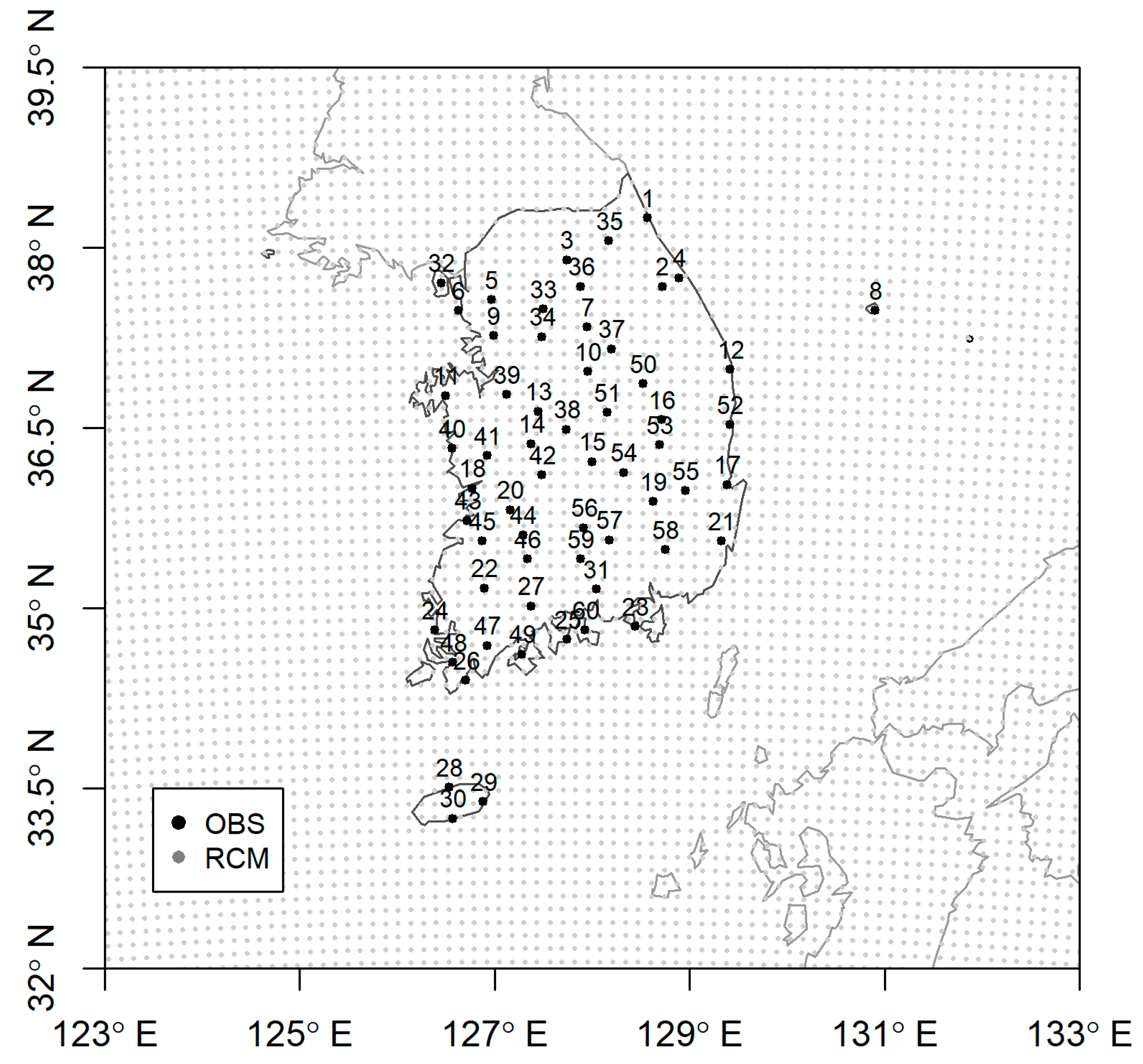
2.3.2. Observed Data
2.3.3. Case Study Methodology
3. Results
4. Discussion
5. Conclusions
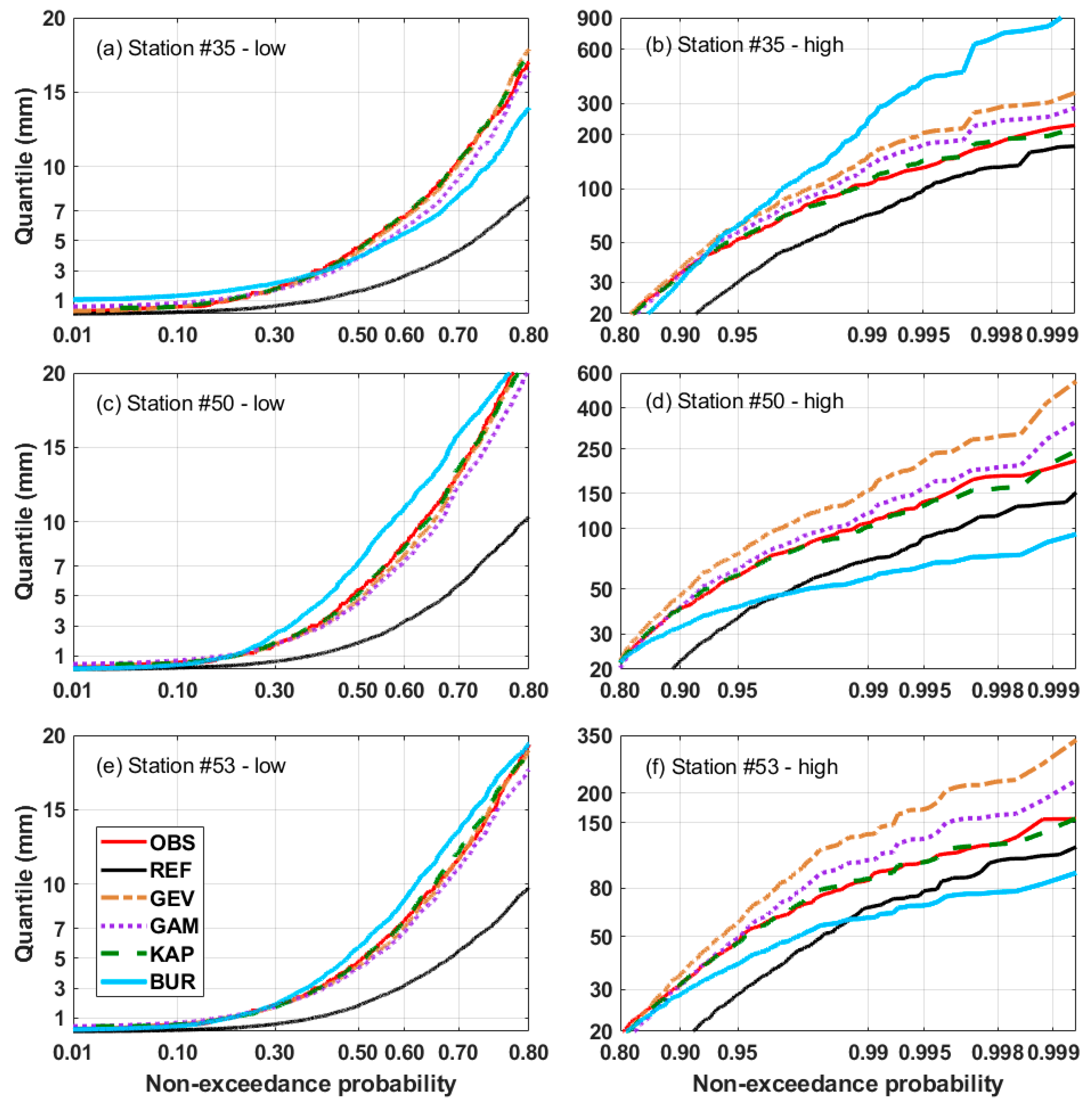
- Two-shape parameter distributions can be used in QDM for a bias correction of the daily precipitation data. The application of GLD and KAP distributions provide good performances in reproducing the statistical characteristics of observed precipitation data, while BUR leads to poor performance. KAP outperforms GAM, which is popularly used in QDM. Additionally, the performance of the GLD can be comparable to one of the GAM.
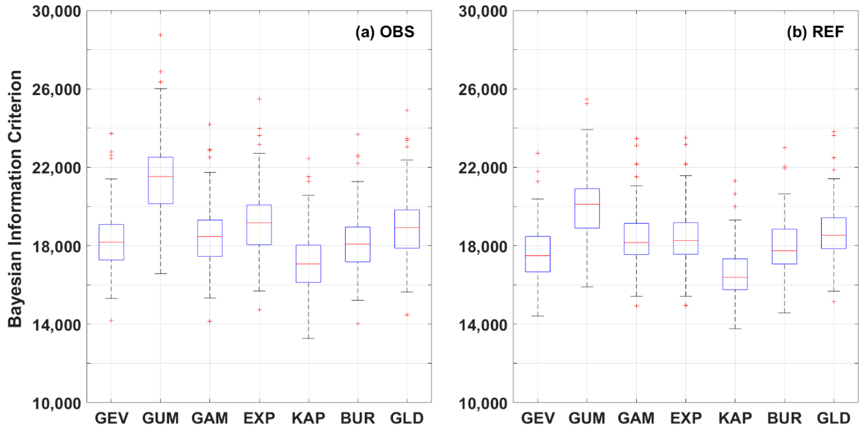
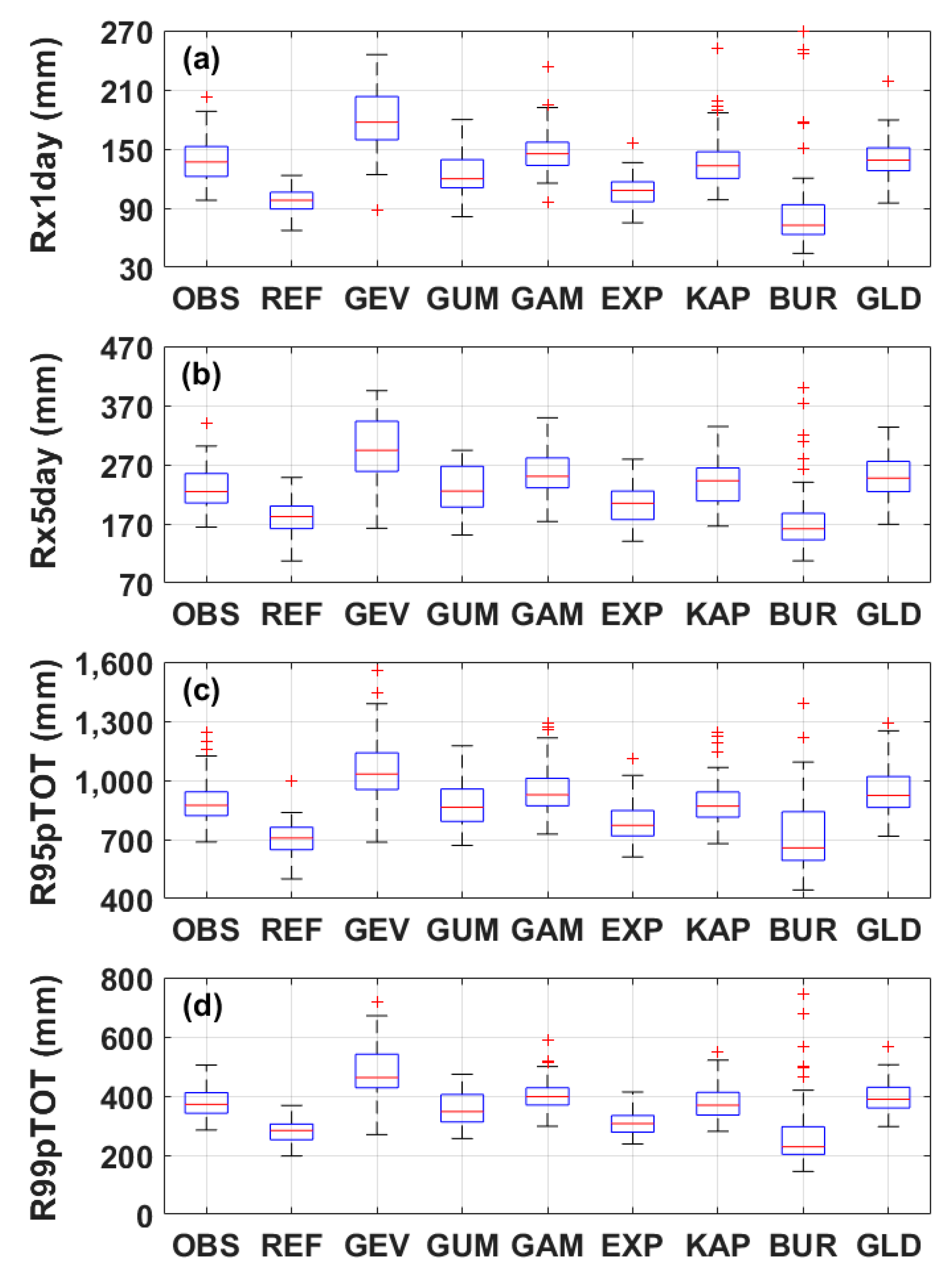
- The KAP distribution is considered as the most appropriate distribution model in QDM for the bias correction of precipitation in South Korea. KAP gives the lowest BIC. Bias-corrected precipitation data using KAP successfully reproduces the basic statistics and extreme characteristics of the observed data. Particularly, KAP is superior to the other distributions for reproducing characteristics of extreme precipitation events.
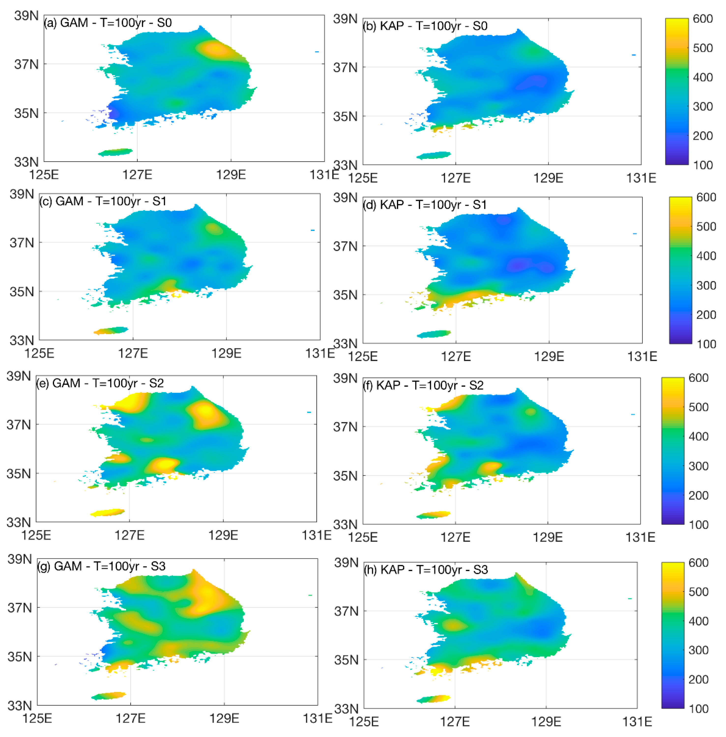
- Selection of an appropriate distribution model in QDM is very important in bias correction of precipitation data. The fit and appropriateness of GAM and KAP are better than that of the other employed distributions based on the results of basic statistics and ETCCDI indices. Results of frequency analysis for extreme precipitation bias-corrected using GAM and KAP present large differences. The precipitation bias-corrected using GAM seems to lose the spatial dependence of observed data during the S2 period, while precipitation data using KAP seems to preserve spatial dependences. When the precipitation data bias-corrected by the GAM are used for flood modeling considering climate change, the result can greatly influence the flood modeling results.
Author Contributions
Funding
Conflicts of Interest
References
- Hagemann, S.; Chen, C.; Haerter, J.O.; Heinke, J.; Gerten, D.; Piani, C. Impact of a Statistical Bias Correction on the Projected Hydrological Changes Obtained from Three GCMs and Two Hydrology Models. J. Hydrometeorol. 2011, 12, 556–578. [Google Scholar] [CrossRef]
- Sillmann, J.; Kharin, V.V.; Zhang, X.; Zwiers, F.W.; Bronaugh, D. Climate extremes indices in the CMIP5 multimodel ensemble: Part 1. Model evaluation in the present climate. J. Geophys. Res. Atmos. 2013, 118, 1716–1733. [Google Scholar] [CrossRef]
- Wilby, R.L.; Hay, L.E.; Gutowski, W.J., Jr.; Arritt, R.W.; Takle, E.S.; Pan, Z.; Leavesley, G.H.; Clark, M.P. Hydrological responses to dynamically and statistically downscaled climate model output. Geophys. Res. Lett. 2000, 27, 1199–1202. [Google Scholar] [CrossRef] [Green Version]
- Wood, A.W.; Leung, L.R.; Sridhar, V.; Lettenmaier, D.P. Hydrologic Implications of Dynamical and Statistical Approaches to Downscaling Climate Model Outputs. Clim. Chang. 2004, 62, 189–216. [Google Scholar] [CrossRef]
- Piani, C.; Weedon, G.P.; Best, M.; Gomes, S.M.; Viterbo, P.; Hagemann, S.; Haerter, J.O. Statistical bias correction of global simulated daily precipitation and temperature for the application of hydrological models. J. Hydrol. 2010, 395, 199–215. [Google Scholar] [CrossRef]
- Eden, J.M.; Widmann, M.; Grawe, D.; Rast, S. Skill, Correction, and Downscaling of GCM-Simulated Precipitation. J. Clim. 2012, 25, 3970–3984. [Google Scholar] [CrossRef] [Green Version]
- Teng, J.; Potter, N.J.; Chiew, F.H.S.; Zhang, L.; Wang, B.; Vaze, J.; Evans, J.P. How does bias correction of regional climate model precipitation affect modelled runoff? Hydrol. Earth Syst. Sci. 2015, 19, 711–728. [Google Scholar] [CrossRef] [Green Version]
- Teutschbein, C.; Seibert, J. Bias correction of regional climate model simulations for hydrological climate-change impact studies: Review and evaluation of different methods. J. Hydrol. 2012, 456, 12–29. [Google Scholar] [CrossRef]
- Gudmundsson, L.; Bremnes, J.B.; Haugen, J.E.; Engen-Skaugen, T. Technical Note: Downscaling RCM precipitation to the station scale using statistical transformations & ndash; a comparison of methods. Hydrol. Earth Syst. Sci. 2012, 16, 3383–3390. [Google Scholar] [CrossRef]
- Chen, J.; Brissette, F.P.; Chaumont, D.; Braun, M. Finding appropriate bias correction methods in downscaling precipitation for hydrologic impact studies over North America. Water Resour. Res. 2013, 49, 4187–4205. [Google Scholar] [CrossRef]
- Themeßl, M.J.; Gobiet, A.; Leuprecht, A. Empirical-statistical downscaling and error correction of daily precipitation from regional climate models. Int. J. Climatol. 2011, 31, 1530–1544. [Google Scholar] [CrossRef]
- Cannon, A.J.; Sobie, S.R.; Murdock, T.Q. Bias Correction of GCM Precipitation by Quantile Mapping: How Well Do Methods Preserve Changes in Quantiles and Extremes? J. Clim. 2015, 28, 6938–6959. [Google Scholar] [CrossRef]
- Buishand, T.A. Some remarks on the use of daily rainfall models. J. Hydrol. 1978, 36, 295–308. [Google Scholar] [CrossRef]
- Geng, S.; Penning de Vries, F.W.T.; Supit, I. A simple method for generating daily rainfall data. Agric. For. Meteorol. 1986, 36, 363–376. [Google Scholar] [CrossRef]
- Schoof, J.T.; Pryor, S.C.; Surprenant, J. Development of daily precipitation projections for the United States based on probabilistic downscaling. J. Geophys. Res. Atmos. 2010, 115. [Google Scholar] [CrossRef]
- Woolhiser, D.A.; Roldán, J. Stochastic daily precipitation models: 2. A comparison of distributions of amounts. Water Resour. Res. 1982, 18, 1461–1468. [Google Scholar] [CrossRef] [Green Version]
- Burgueño, A.; Martínez, M.D.; Lana, X.; Serra, C. Statistical distributions of the daily rainfall regime in Catalonia (Northeastern Spain) for the years 1950–2000. Int. J. Climatol. 2005, 25, 1381–1403. [Google Scholar] [CrossRef]
- Shin, J.-Y.; Lee, T.; Park, T.; Kim, S. Bias correction of RCM outputs using mixture distributions under multiple extreme weather influences. Theor. Appl. Climatol. 2018. [Google Scholar] [CrossRef]
- Papalexiou, S.M.; Koutsoyiannis, D. Entropy based derivation of probability distributions: A case study to daily rainfall. Adv. Water Resour. 2012, 45, 51–57. [Google Scholar] [CrossRef]
- Ye, L.; Hanson, L.S.; Ding, P.; Wang, D.; Vogel, R.M. The probability distribution of daily precipitation at the point and catchment scales in the United States. Hydrol. Earth Syst. Sci. 2018, 22, 6519–6531. [Google Scholar] [CrossRef] [Green Version]
- Howard, T.; Clark, P. Correction and downscaling of NWP wind speed forecasts. Meteorol. Appl. 2007, 14, 105–116. [Google Scholar] [CrossRef]
- Willems, P.; Guillou, A.; Beirlant, J. Bias correction in hydrologic GPD based extreme value analysis by means of a slowly varying function. J. Hydrol. 2007, 338, 221–236. [Google Scholar] [CrossRef]
- Jeon, S.; Paciorek, C.J.; Wehner, M.F. Quantile-based bias correction and uncertainty quantification of extreme event attribution statements. Weather Clim. Extrem. 2016, 12, 24–32. [Google Scholar] [CrossRef] [Green Version]
- Boé, J.; Terray, L.; Habets, F.; Martin, E. Statistical and dynamical downscaling of the Seine basin climate for hydro-meteorological studies. Int. J. Climatol. 2007, 27, 1643–1655. [Google Scholar] [CrossRef]
- Abatzoglou, J.T.; Brown, T.J. A comparison of statistical downscaling methods suited for wildfire applications. Int. J. Climatol. 2012, 32, 772–780. [Google Scholar] [CrossRef]
- Hwang, S.; Graham, W.D. Development and comparative evaluation of a stochastic analog method to downscale daily GCM precipitation. Hydrol. Earth Syst. Sci. 2013, 17, 4481–4502. [Google Scholar] [CrossRef] [Green Version]
- Eum, H.-I.; Simonovic, S.P.; Kim, Y.-O. Climate Change Impact Assessment Using K-Nearest Neighbor Weather Generator: Case Study of the Nakdong River Basin in Korea. J. Hydrol. Eng. 2010, 15, 772–785. [Google Scholar] [CrossRef]
- Seo, S.B.; Kim, Y.-O. Impact of Spatial Aggregation Level of Climate Indicators on a National-Level Selection for Representative Climate Change Scenarios. Sustainability 2018, 10, 2409. [Google Scholar] [CrossRef]
- Eum, H.-I.; Cannon, A.J. Intercomparison of projected changes in climate extremes for South Korea: Application of trend preserving statistical downscaling methods to the CMIP5 ensemble. Int. J. Climatol. 2017, 37, 3381–3397. [Google Scholar] [CrossRef]
- Eagleson, P.S. Dynamics of flood frequency. Water Resour. Res. 1972, 8, 878–898. [Google Scholar] [CrossRef]
- Serinaldi, F. A multisite daily rainfall generator driven by bivariate copula-based mixed distributions. J. Geophys. Res. Atmos. 2009, 114, D10103. [Google Scholar] [CrossRef]
- Kim, D.; Kwon, H.-H.; Lee, S.-O.; Kim, S. Regionalization of the Modified Bartlett–Lewis rectangular pulse stochastic rainfall model across the Korean Peninsula. J. Hydro Environ. Res. 2016, 11, 123–137. [Google Scholar] [CrossRef]
- Sunyer, M.A.; Madsen, H.; Ang, P.H. A comparison of different regional climate models and statistical downscaling methods for extreme rainfall estimation under climate change. Atmos. Res. 2012, 103, 119–128. [Google Scholar] [CrossRef]
- Rodriguez-Iturbe, I.; Cox, D.R.; Isham, V. A point process model for rainfall: Further developments. Proceedings of the Royal Society of London. Math. Phys. Sci. 1988, 417, 283–298. [Google Scholar] [CrossRef]
- Onof, C.; Wheater, H.S. Improvements to the modelling of British rainfall using a modified Random Parameter Bartlett-Lewis Rectangular Pulse Model. J. Hydrol. 1994, 157, 177–195. [Google Scholar] [CrossRef]
- Vrac, M.; Naveau, P. Stochastic downscaling of precipitation: From dry events to heavy rainfalls. Water Resour. Res. 2007, 43. [Google Scholar] [CrossRef] [Green Version]
- Ben-Gai, T.; Bitan, A.; Manes, A.; Alpert, P.; Rubin, S. Spatial and Temporal Changes in Rainfall Frequency Distribution Patterns in Israel. Theor. Appl. Climatol. 1998, 61, 177–190. [Google Scholar] [CrossRef]
- Ines, A.V.M.; Hansen, J.W. Bias correction of daily GCM rainfall for crop simulation studies. Agric. For. Meteorol. 2006, 138, 44–53. [Google Scholar] [CrossRef] [Green Version]
- Piani, C.; Haerter, J.O.; Coppola, E. Statistical bias correction for daily precipitation in regional climate models over Europe. Theor. Appl. Climatol. 2010, 99, 187–192. [Google Scholar] [CrossRef]
- Martins, E.S.; Stedinger, J.R. Generalized maximum-likelihood generalized extreme-value quantile estimators for hydrologic data. Water Resour. Res. 2000, 36, 737–744. [Google Scholar] [CrossRef]
- Katz, R.W.; Parlange, M.B.; Naveau, P. Statistics of extremes in hydrology. Adv. Water Resour. 2002, 25, 1287–1304. [Google Scholar] [CrossRef] [Green Version]
- Nam, W.; Shin, H.; Jung, Y.; Joo, K.; Heo, J.-H. Delineation of the climatic rainfall regions of South Korea based on a multivariate analysis and regional rainfall frequency analyses. Int. J. Climatol. 2015, 35, 777–793. [Google Scholar] [CrossRef]
- Kjeldsen, T.R.; Ahn, H.; Prosdocimi, I.; Heo, J.-H. Mixture Gumbel models for extreme series including infrequent phenomena. Hydrol. Sci. J. 2018, 63, 1927–1940. [Google Scholar] [CrossRef] [Green Version]
- Shin, J.-Y.; Lee, T.; Ouarda, T.B.M.J. Heterogeneous Mixture Distributions for Modeling Multi-source Extreme Rainfalls. J. Hydrometeorol. 2015, 16, 2639–2657. [Google Scholar] [CrossRef]
- Jung, Y.; Shin, J.-Y.; Ahn, H.; Heo, J.-H. The Spatial and Temporal Structure of Extreme Rainfall Trends in South Korea. Water 2017, 9, 809. [Google Scholar] [CrossRef]
- Wallis, J.R.; Schaefer, M.G.; Barker, B.L.; Taylor, G.H. Regional precipitation-frequency analysis and spatial mapping for 24-h and 2-h durations for Washington State. Hydrol. Earth Syst. Sci. 2007, 11, 415–442. [Google Scholar] [CrossRef]
- Parida, B.P. Modelling of Indian summer monsoon rainfall using a four-parameter Kappa distribution. Int. J. Climatol. 1999, 19, 1389–1398. [Google Scholar] [CrossRef]
- Shao, Q.; Wong, H.; Xia, J.; Ip, W.-C. Models for extremes using the extended three-parameter Burr XII system with application to flood frequency analysis/Modèles d’extrêmes utilisant le système Burr XII étendu à trois paramètres et application à l’analyse fréquentielle des crues. Hydrol. Sci. J. 2004, 49, null-702. [Google Scholar] [CrossRef]
- Nadarajah, S.; Bakouch, H.S.; Tahmasbi, R. A generalized Lindley distribution. Sankhya B 2011, 73, 331–359. [Google Scholar] [CrossRef]
- Ganora, D.; Laio, F. Hydrological Applications of the Burr Distribution: Practical Method for Parameter Estimation. J. Hydrol. Eng. 2015, 20, 04015024. [Google Scholar] [CrossRef]
- Norbiato, D.; Borga, M.; Sangati, M.; Zanon, F. Regional frequency analysis of extreme precipitation in the eastern Italian Alps and the August 29, 2003 flash flood. J. Hydrol. 2007, 345, 149–166. [Google Scholar] [CrossRef]
- Park, J.-S.; Jung, H.-S. Modelling Korean extreme rainfall using a Kappa distribution and maximum likelihood estimate. Theor. Appl. Climatol. 2002, 72, 55–64. [Google Scholar] [CrossRef]
- Im, E.-S.; Choi, Y.-W.; Ahn, J.-B. Robust intensification of hydroclimatic intensity over East Asia from multi-model ensemble regional projections. Theor. Appl. Climatol. 2017, 129, 1241–1254. [Google Scholar] [CrossRef]
- Kim, G.; Cha, D.-H.; Park, C.; Lee, G.; Jin, C.-S.; Lee, D.-K.; Suh, M.-S.; Ahn, J.-B.; Min, S.-K.; Hong, S.-Y.; et al. Future changes in extreme precipitation indices over Korea. Int. J. Climatol. 2018, 38, 862–874. [Google Scholar] [CrossRef]
- Giorgi, F.; Jones, C.; Asrar, G.R. Addressing climate information needs at the regional level: The CORDEX framework. World Meteorol. Organ. Bull. 2009, 58, 175. [Google Scholar]
- Oh, S.-G.; Suh, M.-S. Changes in seasonal and diurnal precipitation types during summer over South Korea in the late twenty-first century (2081–2100) projected by the RegCM4.0 based on four RCP scenarios. Clim. Dyn. 2018, 51, 3041–3060. [Google Scholar] [CrossRef]
- Change, I.C. The Physical Science Basis. Contribution of Working Group I to the Fourth Assessment Report of the Intergovernmental Panel on Climate Change; IPCC: Geneva, Switzerland, 2007; p. 996. [Google Scholar]
- Hanson, C.E.; Palutikof, J.P.; Livermore, M.T.J.; Barring, L.; Bindi, M.; Corte-Real, J.; Durao, R.; Giannakopoulos, C.; Good, P.; Holt, T.; et al. Modelling the impact of climate extremes: An overview of the MICE project. Clim. Chang. 2007, 81, 163–177. [Google Scholar] [CrossRef]
- Giorgi, F.; Gutowski, W.J., Jr. Regional Dynamical Downscaling and the CORDEX Initiative. Annu. Rev. Environ. Resour. 2015, 40, 467–490. [Google Scholar] [CrossRef]
- Mearns, L.O.; Arritt, R.; Biner, S.; Bukovsky, M.S.; McGinnis, S.; Sain, S.; Caya, D.; Correia, J., Jr.; Flory, D.; Gutowski, W.; et al. The North American Regional Climate Change Assessment Program: Overview of Phase I Results. Bull. Am. Meteorol. Soc. 2012, 93, 1337–1362. [Google Scholar] [CrossRef]
- Giorgi, F.; Coppola, E.; Solmon, F.; Mariotti, L.; Sylla, M.B.; Bi, X.; Elguindi, N.; Diro, G.T.; Nair, V.; Giuliani, G.; et al. RegCM4: Model description and preliminary tests over multiple CORDEX domains. Clim. Res. 2012, 52, 7–29. [Google Scholar] [CrossRef]
- Skamarock, W.C.; Klemp, J.B.; Dudhia, J.; Gill, D.O.; Barker, D.M.; Wang, W.; Powers, J.G. A Description of the Advanced Research WRF Version 2; National Center for Atmospheric Research Boulder Co Mesoscale and Microscale Div: Boulder, CO, USA, 2005. [Google Scholar]
- So, B.-J.; Kim, J.-Y.; Kwon, H.-H.; Lima, C.H.R. Stochastic extreme downscaling model for an assessment of changes in rainfall intensity-duration-frequency curves over South Korea using multiple regional climate models. J. Hydrol. 2017, 553, 321–337. [Google Scholar] [CrossRef]
- Park, C.; Min, S.-K.; Lee, D.; Cha, D.-H.; Suh, M.-S.; Kang, H.-S.; Hong, S.-Y.; Lee, D.-K.; Baek, H.-J.; Boo, K.-O.; et al. Evaluation of multiple regional climate models for summer climate extremes over East Asia. Clim. Dyn. 2016, 46, 2469–2486. [Google Scholar] [CrossRef]
- Kim, S.; Shin, J.-Y.; Ahn, H.; Heo, J.-H. Selecting Climate Models to Determine Future Extreme Rainfall Quantiles. J. Korean Soc. Hazard Mitig. 2019, 19, 55–69. [Google Scholar] [CrossRef]
- Wingo, D.R. Maximum likelihood methods for fitting the burr type XII distribution to multiply (progressively) censored life test data. Metrika 1993, 40, 203–210. [Google Scholar] [CrossRef]
- Hamed, K.; Rao, A.R. Flood Frequency Analysis; Taylor & Francis: Milton Park, UK, 2010. [Google Scholar]
- Hosking, J.R.M. The four-parameter kappa distribution. IBM J. Res. Dev. 1994, 38, 251–258. [Google Scholar] [CrossRef]
- Vogel, R.M.; Fennessey, N.M. L moment diagrams should replace product moment diagrams. Water Resour. Res. 1993, 29, 1745–1752. [Google Scholar] [CrossRef]
- Kjeldsen, T.R.; Ahn, H.; Prosdocimi, I. On the use of a four-parameter kappa distribution in regional frequency analysis. Hydrol. Sci. J. 2017, 62, 1354–1363. [Google Scholar] [CrossRef] [Green Version]
- Karl, T.R.; Nicholls, N.; Ghazi, A. CLIVAR/GCOS/WMO Workshop on Indices and Indicators for Climate Extremes Workshop Summary. In Weather and Climate Extremes: Changes, Variations and a Perspective from the Insurance Industry; Karl, T.R., Nicholls, N., Ghazi, A., Eds.; Springer: Dordrecht, The Netherlands, 1999; pp. 3–7. [Google Scholar]
- Kim, K.; Kim, N.W.; Kim, D.P.; Park, S.-S.; Won, Y.S.; Lee, D.; Kim, S.; Heo, J.H.; Choi, Y. Survey Report of Water Resource Management Method Development in 1999: Drawing Korean Probability Rainfall Map; Ministry of Construction & Transportation (MOCT): Gwacheon, Korea, 2000. [Google Scholar]
- Hosking, J.R.M.; Wallis, J. Regional Frequency Analysis: An Approach Based on L-Moments; Cambridge University Press: Cambridge, UK, 2005. [Google Scholar]
- Kjeldsen, T.R.; Prosdocimi, I. A bivariate extension of the Hosking and Wallis goodness-of-fit measure for regional distributions. Water Resour. Res. 2015, 51, 896–907. [Google Scholar] [CrossRef]
- Hosking, J.R.M. L-Moments: Analysis and Estimation of Distributions Using Linear Combinations of Order Statistics. J. R. Stat. Soc. Ser. B 1990, 52, 105–124. [Google Scholar] [CrossRef]
- Kay, A.L.; Jones, R.G.; Reynard, N.S. RCM rainfall for UK flood frequency estimation. II. Climate change results. J. Hydrol. 2006, 318, 163–172. [Google Scholar] [CrossRef]
- Blöschl, G.; Hall, J.; Parajka, J.; Perdigão, R.A.P.; Merz, B.; Arheimer, B.; Aronica, G.T.; Bilibashi, A.; Bonacci, O.; Borga, M.; et al. Changing climate shifts timing of European floods. Science 2017, 357, 588–590. [Google Scholar] [CrossRef] [PubMed] [Green Version]
- Dai, A. Increasing drought under global warming in observations and models. Nat. Clim. Chang. 2012, 3, 52. [Google Scholar] [CrossRef]
- Olesen, J.E.; Carter, T.R.; Díaz-Ambrona, C.H.; Fronzek, S.; Heidmann, T.; Hickler, T.; Holt, T.; Minguez, M.I.; Morales, P.; Palutikof, J.P.; et al. Uncertainties in projected impacts of climate change on European agriculture and terrestrial ecosystems based on scenarios from regional climate models. Clim. Chang. 2007, 81, 123–143. [Google Scholar] [CrossRef]
- Kim, K.B.; Bray, M.; Han, D. An improved bias correction scheme based on comparative precipitation characteristics. Hydrol. Process. 2015, 29, 2258–2266. [Google Scholar] [CrossRef]
- Baek, H.-J.; Kim, M.-K.; Kwon, W.-T. Observed short- and long-term changes in summer precipitation over South Korea and their links to large-scale circulation anomalies. Int. J. Climatol. 2017, 37, 972–986. [Google Scholar] [CrossRef]
- Ben Alaya, M.A.; Ouarda, T.B.M.J.; Chebana, F. Non-Gaussian spatiotemporal simulation of multisite daily precipitation: Downscaling framework. Clim. Dyn. 2017. [Google Scholar] [CrossRef]
- Costa, V.; Fernandes, W.; Naghettini, M. A Bayesian model for stochastic generation of daily precipitation using an upper-bounded distribution function. Stoch. Environ. Res. Risk Assess. 2015, 29, 563–576. [Google Scholar] [CrossRef]
- Hayes, M.J.; Svoboda, M.D.; Wiihite, D.A.; Vanyarkho, O.V. Monitoring the 1996 Drought Using the Standardized Precipitation Index. Bull. Am. Meteorol. Soc. 1999, 80, 429–438. [Google Scholar] [CrossRef] [Green Version]
- Husak, G.J.; Michaelsen, J.; Funk, C. Use of the gamma distribution to represent monthly rainfall in Africa for drought monitoring applications. Int. J. Climatol. 2007, 27, 935–944. [Google Scholar] [CrossRef]
- Seo, D.-J.; Smith, J.A. Rainfall estimation using raingages and radar—A Bayesian approach: 2. An application. Stoch. Hydrol. Hydraul. 1991, 5, 31–44. [Google Scholar] [CrossRef]


| Model | Cumulative Distribution Function |
|---|---|
| Gumbel | |
| Generalized extreme value | |
| Gamma | |
| Exponential | |
| Kappa | |
| Burr XII | |
| Generalized Lindley |
| No. | Name | Latitude | Longitude | No. | Name | Latitude | Longitude |
|---|---|---|---|---|---|---|---|
| 1 | Daegwallyeong | 128.72 | 37.68 | 31 | Yeongdeok | 129.41 | 36.53 |
| 2 | Jecheon | 128.19 | 37.16 | 32 | Pohang | 129.38 | 36.03 |
| 3 | Chungju | 127.95 | 36.97 | 33 | Namhae | 127.93 | 34.82 |
| 4 | Wonju | 127.95 | 37.34 | 34 | Tongyeong | 128.44 | 34.85 |
| 5 | Yangpyeong | 127.49 | 37.49 | 35 | Geumsan | 127.48 | 36.11 |
| 6 | Icheon | 127.48 | 37.26 | 36 | Chupungnyeong | 127.99 | 36.22 |
| 7 | Inje | 128.17 | 38.06 | 37 | Boeun | 127.73 | 36.49 |
| 8 | Chuncheon | 127.74 | 37.90 | 38 | Daejeon | 127.37 | 36.37 |
| 9 | Hongcheon | 127.88 | 37.68 | 39 | Cheongju | 127.44 | 36.64 |
| 10 | Seoul | 126.97 | 37.57 | 40 | Buyeo | 126.92 | 36.27 |
| 11 | Suwon | 126.99 | 37.27 | 41 | Cheonan | 127.12 | 36.78 |
| 12 | Incheon | 126.63 | 37.48 | 42 | Seosan | 126.50 | 36.77 |
| 13 | Ganghwa | 126.45 | 37.71 | 43 | Gunsan | 126.76 | 36.00 |
| 14 | Sokcho | 128.57 | 38.25 | 44 | Boryeong | 126.56 | 36.33 |
| 15 | Gangneung | 128.89 | 37.75 | 45 | Jeonju | 127.16 | 35.82 |
| 16 | Andong | 128.71 | 36.57 | 46 | Jeongeup | 126.87 | 35.56 |
| 17 | Yeongju | 128.52 | 36.87 | 47 | Buan | 126.72 | 35.73 |
| 18 | Mungyeong | 128.15 | 36.63 | 48 | Imsil | 127.29 | 35.61 |
| 19 | Uiseong | 128.69 | 36.36 | 49 | Namwon | 127.33 | 35.41 |
| 20 | Gumi | 128.32 | 36.13 | 50 | Wando | 126.70 | 34.40 |
| 21 | Daegu | 128.62 | 35.89 | 51 | Suncheon | 127.37 | 35.02 |
| 22 | Yeongcheon | 128.95 | 35.98 | 52 | Goheung | 127.28 | 34.62 |
| 23 | Geochang | 127.91 | 35.67 | 53 | Yoesu | 127.74 | 34.74 |
| 24 | Hapcheon | 128.17 | 35.57 | 54 | Gwangju | 126.89 | 35.17 |
| 25 | Sancheong | 127.88 | 35.41 | 55 | Jangheung | 126.92 | 34.69 |
| 26 | Jinju | 128.04 | 35.16 | 56 | Haenam | 126.57 | 34.55 |
| 27 | Miryang | 128.74 | 35.49 | 57 | Mokpo | 126.38 | 34.82 |
| 28 | Ulsan | 129.32 | 35.56 | 58 | Jeju | 126.53 | 33.51 |
| 29 | Ulleungdo | 130.90 | 37.48 | 59 | Seogwipo | 126.57 | 33.25 |
| 30 | Uljin | 129.41 | 36.99 | 60 | Seongsan | 126.88 | 33.39 |
| Acronym | Description | Unit |
|---|---|---|
| Mean | Mean daily precipitation | mm |
| SD | Standard deviation of daily precipitation | mm |
| CS | Coefficient of skewness of daily precipitation | - |
| PRCPTOT | Annual total precipitation in wet days (daily precipitation ≥ 1 mm) | mm |
| SDII | Annual precipitation divided by the number of wet days | mm/day |
| Rx1day | Annual maximum 1-day precipitation | mm |
| Rx5day | Annual maximum 5-day precipitation | mm |
| R95pTOT | Annual total rainfall when daily precipitation > 95 percentile | mm |
| R99pTOT | Annual total rainfall when daily precipitation > 99 percentile | mm |
| Distributions | Observed Data | Simulated Data | ||||
|---|---|---|---|---|---|---|
| 1st | 2nd | 3rd | 1st | 2nd | 3rd | |
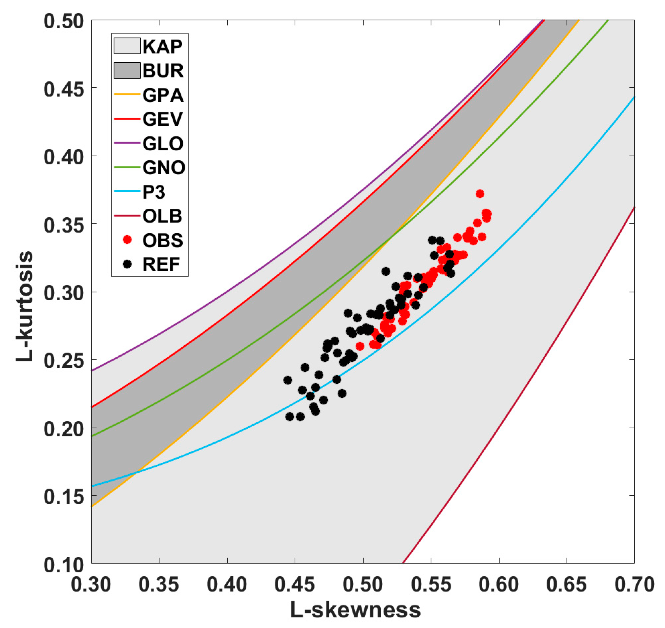
| GEV | - | 9 (15%) | 38 (63%) | - | 60 (100%) | - |
| GUM | - | - | - | - | - | - |
| GAM | - | - | 13 (22%) | - | - | 1 (2%) |
| EXP | - | - | - | - | - | - |
| KAP | 60 (100%) | - | - | 60 (100%) | - | - |
| BUR | - | 51 (85%) | 9 (15%) | - | - | 59 (98%) |
| GLD | - | - | - | - | - | - |
© 2019 by the authors. Licensee MDPI, Basel, Switzerland. This article is an open access article distributed under the terms and conditions of the Creative Commons Attribution (CC BY) license (http://creativecommons.org/licenses/by/4.0/).
Share and Cite
Heo, J.-H.; Ahn, H.; Shin, J.-Y.; Kjeldsen, T.R.; Jeong, C. Probability Distributions for a Quantile Mapping Technique for a Bias Correction of Precipitation Data: A Case Study to Precipitation Data Under Climate Change. Water 2019, 11, 1475. https://doi.org/10.3390/w11071475
Heo J-H, Ahn H, Shin J-Y, Kjeldsen TR, Jeong C. Probability Distributions for a Quantile Mapping Technique for a Bias Correction of Precipitation Data: A Case Study to Precipitation Data Under Climate Change. Water. 2019; 11(7):1475. https://doi.org/10.3390/w11071475
Chicago/Turabian StyleHeo, Jun-Haeng, Hyunjun Ahn, Ju-Young Shin, Thomas Rodding Kjeldsen, and Changsam Jeong. 2019. "Probability Distributions for a Quantile Mapping Technique for a Bias Correction of Precipitation Data: A Case Study to Precipitation Data Under Climate Change" Water 11, no. 7: 1475. https://doi.org/10.3390/w11071475