Microplastics in a Stormwater Pond


Department of Civil Engineering, Aalborg University, Thomas Manns Vej 23, 9220 Aalborg Øst, Denmark
*
Author to whom correspondence should be addressed.
Water 2019, 11(7), 1466; https://doi.org/10.3390/w11071466
Submission received: 3 June 2019
/
Revised: 28 June 2019
/
Accepted: 2 July 2019
/
Published: 15 July 2019
(This article belongs to the Special Issue Stormwater Management in Cool and Cold Climates)
Abstract
:Large amounts of microplastics (MPs) enter our environment through runoff from urban areas. This study presents results for MPs in stormwater from a wet retention pond in terms of its water, sediments, and vertebrate fauna. The analysis was done for the size range 10–500 μm, applying a focal-plane array-based µFourier transform infrared (FPA-µFTIR) imaging technique with automated data analysis. Sample preparation protocols were optimized towards this analytical method. The study revealed 270 item L−1 in the pond water, corresponding to 4.2 µg L−1. The MPs in the pond were highly concentrated in its sediments, reaching 0.4 g kg−1, corresponding to nearly 106 item kg−1. MPs also accumulated in vertebrates from the pond—three-spined sticklebacks and young newts. In terms of particle numbers, this accumulation reached levels nearly as high as in the sediments. The size of the MPs in the pond water and its fauna was quite similar and significantly smaller than the MPs in the sediments. A rough estimate on MPs retention in the pond indicated that MPs were retained at efficiencies similar to that of other particulate materials occurring in the stormwater runoff.
1. Introduction
Microplastics (MPs) in the marine environment originate mainly from land-based sources and reach it by direct transport with runoff and by weathering of larger plastic debris [1,2]. There is also a less well-understood contribution from atmospheric deposition, documented by findings of MPs in outdoor air [3]. However, the relative contribution of the various land-based MPs sources and their pathways to the environment are not well understood, leaving numerous uncertainties regarding which sources are dominant [4]. MPs are present in lakes and rivers, showing that freshwaters receive MPs from land-based sources and also transport MPs to the oceans [5,6]. Urban activities and population densities have been shown to affect the occurrence of MPs in rivers. For example, a recent study of 29 Japanese rivers revealed a correspondence between general pollutant parameters and the MPs content [7]. Studies in the Canadian part of Lake Ontario have shown similar results, concluding that MPs concentration levels increase close to urban and industrial areas [8].
One urban MPs source is wastewater discharges. Wastewater receives contributions from households and industries, as well as from surface runoff in combined sewer networks. A number of studies have pointed out that especially untreated wastewater can be a substantial source of MPs, while treated wastewater still contains MPs, but at much lower concentrations [9,10,11]. MP concentrations in untreated Danish wastewater have been reported to be about 250 µg L−1, which corresponds to 191 t MPs annually entering Danish treatment plants [11]. Taking the treatment efficiency of the plants into account, the calculated annual MPs discharge to the aquatic environment is 3 t MPs. Another urban source for MPs is the built environment itself and the activities on its surfaces. Several authors have concluded that treated wastewater alone cannot explain the occurrence of MPs in urban waters, and that stormwater runoff from impervious surfaces must contribute [12,13].
It is problematic to compare the various reports on MPs occurrences, though. The main reasons being that different analytical approaches have been used for quantification of MPs, that sampling approaches differ, and that the lower size limit of detection and quantification varies between studies (e.g., [14,15]). Another contributing factor is that the accuracy of quantification is seldom determined, leaving it uncertain whether some studies have actually captured all MPs in the targeted size range, or whether non-plastic particles have been misinterpreted as MPs [16,17,18]. Comparing studies is further complicated by the fact that the vast majority report MPs in terms of particle number per unit volume or unit mass, which makes it inherently difficult to compare studies as particles are brittle and disintegrate over time. In other words, particle concentration in terms of numbers is not a conserved quantity [2,11,19,20]. While particle numbers are very important when assessing the environmental impacts of MPs, this measure is insufficient when assessing the load of MPs in the environment or the efficiency of treatment practices. Here, the mass of MPs must be used, preferably in combination with particle size distributions. Ref. [11] showed how FPA-µFTIR imaging can be used for this purpose; namely, to quantify both MPs number and mass.
Lately, MPs have been found in the waters of urban and highway retention ponds [21]. These water bodies are small and shallow artificial lakes installed to treat the surface runoff from urban areas and roads. Their morphology is rather similar to other urban water bodies [22], but their technical purpose is flood mitigation and treatment of polluted runoff. Even though they are intended as technical treatment solutions, they do more than retain pollutants by simple settling processes, as they also sequestrate carbon and retain nutrients by biological processes [23]. They become colonized by flora and fauna quite similar to small natural water bodies, establishing ecosystems containing algae, macrophytes, invertebrates, and vertebrates [24,25]. This leads to retention ponds being versatile in terms of their pollutant retainment, and it is likely that they also act as sinks for MPs.
The objective of this investigation was to quantify the distribution of MP in stormwater retention ponds and to explore their potential as MPs sinks. The approach was to study one pond in-depth by quantifying MPs in the water, sediments, and selected fauna. Besides determining concentrations in the different phases, it was the intention to gain knowledge on which particle sizes and plastic types occurred in these matrices. FPA-µFTIR imaging with a focus on the 10 to 500 μm size range was the analytical technique used for quantification. It was an additional objective to optimize protocols for the purification and concentration of MPs from these matrices, and to evaluate the reliability of the analysis in terms of MPs recovery and background contamination.
2. Materials and Method
2.1. Study Area
The investigated stormwater retention pond is more than 30 years old and located in Viborg, Denmark (56°28′29.3″, 9°24′43.3″). It is one of Denmark’s oldest stormwater ponds and was dredged for sediments 10 to 15 years ago. Visually, it appears similar to a small natural lake (Figure 1), with a surface area of 6690 m2 and a total volume of approximately 7500 m3. It serves a drainage area of 166 ha, of which 70 ha are impervious and thus contributing to the runoff. The annual precipitation in Viborg is 800 mm, according to national meteorological data. A reasonable estimate of the hydrological reduction factor needed to calculate the runoff for such a catchment is 0.5 [26], meaning that half of the precipitation falling on the impervious area will end up as runoff entering the pond. The average inflow to the pond is thus approximately 280,000 m3 yr−1, corresponding to an average stormwater retention time of roughly 10 days. The drainage area can be described as light industry and includes production industries, retailers, building supply stores, parking lots, as well as roads with semi-heavy traffic. Additionally, plastic litter can be observed along the eastern side of the pond, where a path runs through the area.
2.2. Sampling
Samples of sediments, water, and fauna were collected from September to December 2016 at the locations shown in Figure 1. The general pollutant content of stormwater runoff is known to vary significantly during events and between events (e.g., [27,28]), causing the pollutant concentration in the water phase of stormwater ponds to vary correspondingly [25,29]. To compensate for short-term variations in bulk water concentrations, the water was sampled 5 times during dry weather and with a minimum of 14 days between samplings. At each sampling, 10 L was collected, totaling 50 L of pond water. Each batch was stored in 2 × 5 L glass storage bottles with Teflon-coated (Polytetrafluoroethylene, PTFE) screw caps. The water was sampled 2 to 3 m out from the shoreline at a water depth of at least 0.5 m. The bottles were flushed with pond water 3 times before the sample was collected 0.1 m below the water surface. Bottles were filled carefully to avoid contamination by sediments. After sampling, the two bottles were brought to the laboratory and stored at 5 °C prior to analysis.
Sediments were sampled in October 2016 by a glass corer with a diameter of 5 cm. Intact cores were collected in the littoral zone, 2 m out from the shoreline and approximately midways between the inlet and outlet of the pond. The top layer of the sediment cores (approximately 5–8 cm) was transferred into a glass jar. Multiple sediment cores were sampled, resulting in a bulk sample of 1 to 2 kg. All jars were stored at 5 °C prior to analysis.
In September 2016, three-spined sticklebacks (Gasterosteus aculeatus) and young newts (Triturus vulgaris) were sampled in quantities suitable for further analysis. The sticklebacks were caught by a 20 m long and 1 m wide surface gill net, which reached from the water surface to 1 m below. The net was placed across the pond and left for 24 h before it was collected and emptied. The fish caught were 2 to 6 cm long with an average size of 4.8 cm and an average wet weight of 6.38 g. The newts were caught with a fishing net from the shore. The newts were 5 to 7 cm long with an average size of 5.9 cm and an average wet weight of 4.61 g. The collected specimens were placed in ethanol, brought to the laboratory, cleaned in Milli-Q water, and stored at −20 °C prior to analysis.
2.3. Analysis
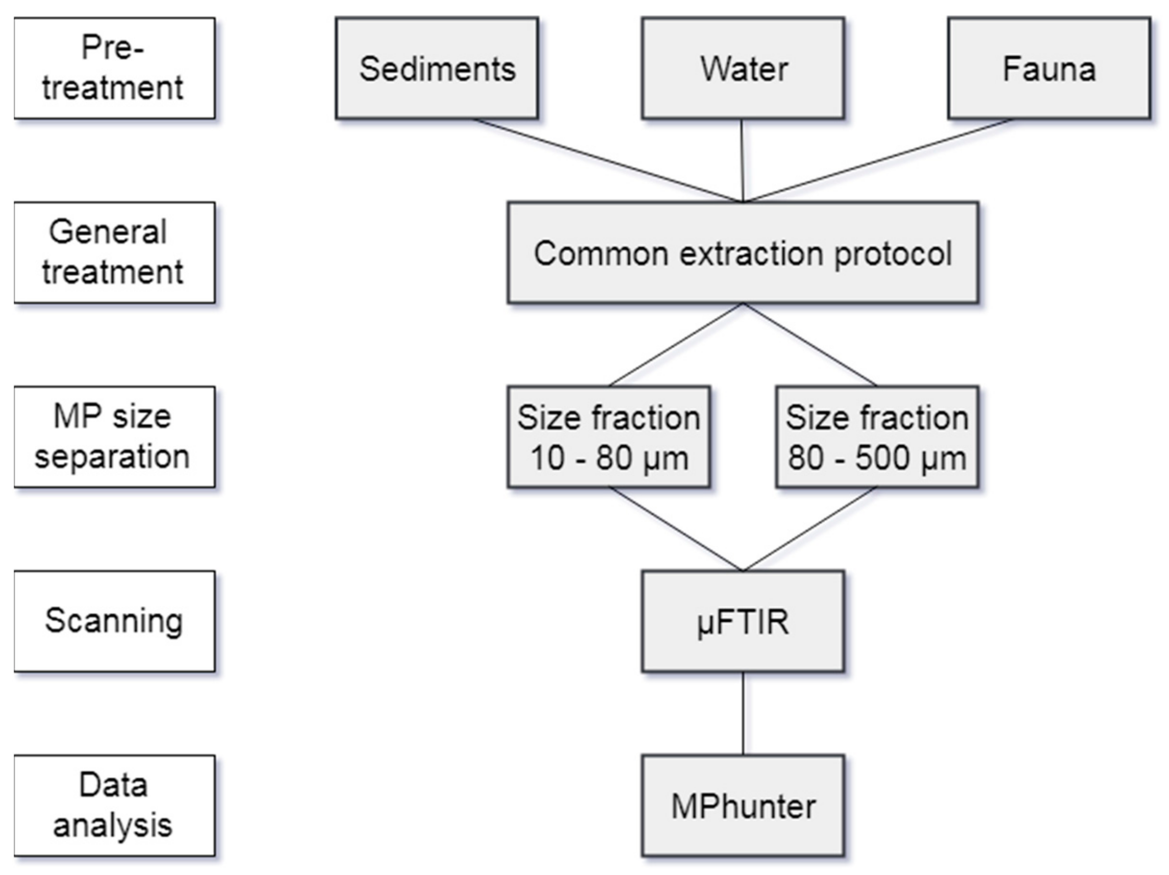
The treatment of the three matrices consisted of individual pre-treatment protocols, followed by a common treatment protocol. The final product was a concentrate of particles suspended in 50% ethanol. The MP in the extracts were quantified by FPA-µFTIR imaging, and the data analysis performed by an automatic MP detection procedure (Figure 2).
2.4. Sediment Extraction Protocol
First, large material, such as sticks, leaves, and gravel, was eliminated from the sample by wet-sieving all sediments through a 2 mm sieve using a 0.15 g L−1 sodium dodecyl sulfate (SDS) solution. A Retsch AS 200 vibratory sieve shaker was used for all wet-sieving. The effluent was collected and settled for a week at room temperature. To reduce the wet volume, most liquid was decanted off and filtered onto a stainless-steel filter with a mesh size of 10 µm (referred to as a 10 µm filter). The particles on the 10 µm filter were removed by 15 min of sonication in Milli-Q and flushed back into the settled sample slurry. The sediment slurry was divided into glass containers and stored at −20 °C before it was freeze-dried.
Upon drying, the sediments were thoroughly mixed, and a subsample of 10 g was taken for further analysis. The sample was suspended in 150 mL Milli-Q and agitated for 15 min before 145 mL of 50% w/w H2O2 was slowly added. The sample was oxidized with slow stirring at 30 °C for 48 h. The inside of the glassware was then flushed before the sample settled for another 48 h. The volume of the suspension was reduced by filtering the liquid onto several 10 µm filters.
The inorganic particles of the sediments and those collected on the filters were removed by gravimetric separation. The separation medium was an 11 M zinc chloride solution (ZnCl2) with a density of 1.7 kg L−1, filtered on a 0.8 µm GF filter. First, the settled sediments were transferred to a straight glass funnel. The sediments on the filters, which were collected during the volume reduction of the sample, were then transferred to the same funnel, using 15 min of sonication in the ZnCl2 solution. The funnel was then topped off with ZnCl2 solution to 600 to 700 mL, upon which the sample was agitated for 30 min by aeration from below. The inside of the funnel was flushed with ZnCl2 solution to recover the particles sticking to the glass wall. The funnel was left for 24 h before the approximately top 8 cm was drained through a side port of the funnel. After refilling the funnel with new ZnCl2 solution, the flotation sequence was repeated. In total, the aeration was repeated 3 times. All liquid obtained from the flotation sequence was then filtered onto a 10 µm filter. The particles on the filter were flushed with Milli-Q and removed by 15 min of sonication in a 0.15 g L−1 SDS solution. The volume of the resuspended particles was then set to 150 mL with a 0.15 g L−1 SDS solution before undergoing the common extraction protocol.
2.5. Common Extraction Protocol
In short, the common extraction protocol consisted of enzymatic digestion with cellulase followed by a Fenton’s oxidation and finally wet-sieving to separate the particles into two size fractions—above and below 80 µm. The protocol developed for raw wastewater by [11] was followed with slight modifications: The Fenton’s reaction was conducted by adding 110 mL 50% w/w H2O2, 48 mL of 0.1 M sodium hydroxide, and 46 mL of 0.1 M iron(II)sulfate to a sample volume of 150 mL. Particle concentrates were stored in 5 mL of a 50% ethanol solution (99% HPLC grade ethanol and 100% LC-MS grade water) instead of pure ethanol. To accelerate the evaporation, the samples were evaporated at 40 °C with a gentle nitrogen flow.
From the particle concentrate, a homogenized subsample was transferred to either a transmission window or a reflection slide. The size fraction above 80 µm was deposited on a MirrIR slide (Kevley Technologies, Chesterland, OH, USA) by fixing a PTFE-coated rubber washer with an inner diameter of 10 mm on top. The size fraction below 80 µm was deposited on a zinc selenide (ZnSe, Crystran Ltd., Dorset, UK) window (13 mm diameter) placed in a compression cell, reducing the diameter to 10 mm. After depositing 100 µL, the substrate (slide or window) was left for drying, and the particle density visually assessed under a microscope. If the deposited particle density was deemed too small, an additional volume was deposited. This procedure was repeated until a suitable particle density was achieved, upon which the substrate was completely dried and stored for chemical analysis.
2.6. Pond Water Extraction Protocol
The 50 L of pond water were filtered on several 10 µm filters and the particles transferred to a 0.15 g L−1 SDS solution by 15 min of sonication. The sonicated filters were rinsed for particulate matter and discharged. The SDS solution containing the particles was collected in a glass bottle and 1 mL of 150 g L−1 SDS was added to counteract particles adhering to the glass wall. The volume was adjusted to 1.5 L by adding Milli-Q. From this concentrate, a 150 mL subsample was taken and introduced to the common extraction protocol.
2.7. Fauna Protocol
The fauna samples were freeze-dried as whole organisms. To digest the soft tissue, the freeze-dried organisms were placed in a beaker where 60 mL of 5 M KOH was added per 1 g of dry weight [30,31,32]. The solution was then stirred and incubated for 48 h at 45 °C. Before terminating the digestion, 100 mL of Milli-Q was added. The solution was stirred for an additional 15 min before the undigested particles were filtered onto a 10 µm filter. To prevent the filter from clogging, the filter was flushed with 0.07 M acetic acid when needed. Finally, the particles on the filter were washed, once with 300 mL 0.07 M acetic acid and twice with 400 mL Milli-Q. The particles on the filter were removed by 15 min of sonication in 0.15 g L−1 SDS. The filter was cleaned and removed, and the volume was adjusted to 150 mL and introduced to the common extraction protocol.
2.8. Data Analysis
The substrate containing the deposited particle concentrates were analyzed by µFTIR imaging, using a Cary 620 FTIR microscope coupled with a Cary 670 FTIR spectrometer (Agilent technologies, Santa Clara, CA, USA). The microscope was operated with a 15× Cassegrain objective and the FPA was a 128 × 128 Mercury Cadmium Telluride (MCT) FPA detector. The resulting pixel resolution was 5.5 μm, yielding approximately 3.2 million individual infrared (IR) spectra per substrate. The scanning settings for the spectral range, resolution, and scanning area were set as described by [11]. The MirrIR reflection slides were scanned in reflection mode and the ZnSe windows were scanned in transmission mode.
Manual analysis of the entire scanned substrate is not feasible, and an automated approach was used. The approach is a modification of the concept presented by [18], where the many individual spectra are analyzed by comparing them to a reference library and building images of MP particles from this. The analysis was done using MPhunter; a software developed at Aalborg University, Aalborg, Denmark, in collaboration with Alfred Wegener Institute, Helgoland, Germany [21]. The customized library applied in MPhunter contained 113 spectra of primarily common polymers and some natural materials. All MP matches were checked manually for false positives and particles were only positively identified as MPs when a confirmation was found in the fingerprint region. The material groups considered in the analysis were: Acrylonitrile butadiene styrene (ABS), acrylic, acrylic paints, alkyd, aramid, cellulose acetate, diene elastomer, ethylene propylene diene monomers (EPDMs), epoxy, ethylene vinyl acetate (EVA), polyamide (PA), polyacrylonitrile (PAN Acrylic), polyethylene (PE), Pebax®, polyethylene glycol (PEG), phenoxy resin, polylactic acid (PLA), polycarbonate, polyester, polyoxymethylene (POM), polypropylene (PP), polystyrene (PS), polytetrafluoroethylene (PTFE), polyurethane (PU), polyurethane paints (PU paints), polyvinyl alcohol (PVA), polyvinyl acetate (PVAC), polyvinyl chloride (PVC), styrene acrylonitrile (SAN), styrene butadiene rubber (SBR), and vinyl copolymer. Due to the use of PTFE-coated rubber washers, sealing materials, and septa, MP particles of this material were eliminated from the results. The applied FTIR-method was not able to identify car tire rubber even though it contains SBR, as the carbon black added to the tire tread absorbs the IR light.
For each MP, the analysis resulted in polymer material and its dimensions. The major dimension was measured along the particles’ longest axis, while the minor dimension was calculated based on the area the particle covered, together with the simplifying assumption that all particles were elliptical [21]. The particle volume was estimated by the assumption that all particles were ellipsoids, with the third dimension being 0.67 times the minor dimension [11]. The calculated MP concentrations were normalized to item and mass per cubic meter (water) and item and mass per solid dry weight (sediments and fauna). Quantifying the major and minor dimensions of MPs also allowed fiber-like particles to be detected. In this study, the length to width ratio applied by [33] was used, where particles with a ratio above 3:1 are characterized as fibers.
MP data were tested with a Shapiro–Wilk test for normal distribution. For multiple comparisons, ANOVA and Tukey tests were used. In all cases, the significance level was set to 0.05. All statistical analysis was performed in the software R (v3.5.1).
2.9. Method Validation
Several precautions were taken to reduce the risk of contamination: Lab coats were worn at all times, all glassware was rinsed 3 times with Milli-Q before use, all equipment was kept covered at all times to minimize airborne contamination, and reagents were filtered on 1.2 µm glass fiber (GF) filters. Plastic materials were avoided unless otherwise stated. All chemicals were of analytical grade and diluted to the desired concentration in Milli-Q. For the 0.15 g L−1 SDS solution, 0.8 µm filtered (mixed cellulose ester filter) demineralized water was used. Furthermore, the air of the µFTIR scanning room was continuously filtered by an air treatment device (Dustbox® Hochleistungsluftreininger, Germany) with a high efficiency particulate air (HEPA) filter (H14, 7.5 m2).
Three blank controls were processed to assess the background contamination from the sample preparation. The blanks consisted of 150 mL Milli-Q water and underwent the protocol described for common extraction.
Recovery tests were performed on all sample matrices by spiking with a known number of red 100 μm PS beads (Sigma-Aldrich, product no. 56969). The spiked samples were processed, and the particles were extracted according to the described protocol. The extracted particles were transferred onto a glass microscope slide, visually identified by their distinct appearance using a Meiji Techno MT4310 trinocular phase microscope, and counted.
2.10. Other Parameters
Total suspended solids (TSSs) and the organic matter (OM) content was analyzed according to [34]. Sediment sieving curves were made on sediments dried at 105 °C for 24 h, following the protocol described in DS/EN ISO 17892-4:2016.
3. Results and Discussion
The collected water samples held 8 mg L−1 of TSSs with an OM content of 66%, which is well within the range of the 167 reservoirs and lakes studied by [35] and in the lower range of typical discharges from stormwater retention ponds and wetlands [36]. The sediments can be described as poorly graded, where 24.4 % of the particles were of a smaller size than 0.063 mm. The sediments of the pond had an organic matter content of 19%, which is in the range of reported organic matter contents for such sediments [37].
All samples contained MPs. In total, 333 particles were identified as MPs by the µFTIR imaging, with 244 MPs in the sediments, 40 in the water, and 41 in the fauna samples. Back-calculating to concentrations, this resulted in the MP numbers and masses as shown in Table 1. The highest concentration was found in the sediments, followed by the fauna and the water. In terms of items per mass of the sample, the sediments held 3500 times more MPs than the water, while the fauna held 1300 times higher concentrations. In other words, the relative MP number concentrations were 3500:1300:1 for sediments, fauna, and water, respectively. With respect to the MPs mass concentrations, the corresponding numbers were 96,000:3100:1. Hence, MPs tended to concentrate in both the sediments and the fauna by several orders of magnitude.
3.1. Contamination and Recovery
Addressing the background contamination is an acknowledged prerequisite when dealing with MP analysis [9,20]. A total of 20 MPs were found in the three blanks. Out of these, 12 were PTFE. Since PTFE was used in the sample preparation and analysis, it was excluded from the data analysis and the blank calculations. The other eight particles were polyester (5), PS (1), ABS (1), and cellulose acetate (1). In terms of mass, polyester constituted 46% of the contamination. For each blank, only a sub-sample of the 5 mL particle concentrate was analyzed, and the calculated average MP concentration in the three blanks was estimated to be 50 item (5 mL particle concentrate)−1 and 3.9 µg (5 mL particle concentrate)−1. Relating these findings to the different samples resulted in the blank concentration shown in Table 1.
The blank concentrations showed that 0.5% of the sediments’ particle concentration and 0.1% of the calculated mass concentration could be related to background contamination. However, the sediment-specific treatment steps were not included in the blank procedure, and the actual background contamination could thus be higher. For the water samples, less MPs were identified and the background contamination was hence somewhat proportionally higher, namely 3.8% and 18.6% for the MP number and mass concentrations, respectively. The fauna samples had the highest uncertainties related to the background contamination, namely 14.9% for the MP number concentration and 30.4% for the MP mass concentration. Data were not corrected for contamination due to the low numbers of MPs found in the blanks and the corresponding uncertainty on the quantification of background contamination in terms of MP numbers, masses, and polymeric composition.
The recovery tests showed that 96% of the added PS beads were recovered by the water protocol, 75% by the fauna protocol, and 64% by the sediment protocol, reflecting that the analysis of the water required less sample preparation steps than the fauna and the sediments. It cannot be ruled out that the 100 µm PS beads have a different recovery compared to some naturally occurring MPs, as the beads were spherical and had not undergone ageing prior to use. It is quite possible that different materials and particle shapes were recovered at different rates, and that the recovery of naturally occurring MPs was better for larger particles and poorer for smaller particles, further contributing to the uncertainties of quantification [38]. Due to these issues, it was not feasible to correct the data (Table 1) for recovery.
3.2. MPs in the Water Phase
The number of studies reporting MPs concentrations in the size range of 10 to 500 µm while also applying spectroscopic confirmation of the material are few, leaving comparisons with previous studies somewhat tenuous. For stormwater ponds, the only study that addressed MPs concentrations is, to the best knowledge of the authors, [21]. They analyzed the water phase of seven stormwater ponds and found MP numbers ranging from 4.9 × 10² to 2.3 × 10⁵ item m−3 and MP masses ranging from 8.5 × 10⁻² to 1.1 mg m−3. The water phase MPs concentrations of the present study were hence near the upper bound of that study. One of the ponds sampled by Liu et al. [21] was the same pond investigated in this study. For that pond, they reported 1.1 × 10⁵ item m−3 and 6.6 × 10⁻¹ mg m−3, i.e., slightly lower than in the present study. Possible explanations for the difference could be that the two studies sampled the pond at different times of the year. Furthermore, it seems quite probable that loadings on the pond have varied with activities in the catchment, leading to fluctuations in pond water MPs concentrations. Another explanation could be that the two studies used different sampling approaches. While samples in the present study were filtered in the lab, Liu et al. [21]. filtered pond water on site. Furthermore, the filtered volumes of that study were approximately 20 times larger than in the present study.
Another study addressing stormwater was presented by [39], who analyzed the particulate phase of highway runoff for SBR (tire wear particles), PE, PP, and PS using thermal decomposition coupled to gas chromatography-mass spectrometry (GC-MS). They found that about 12 mg g−1 of the stormwater particles belonged to PE, PP, and PS, while SBR was present at roughly 28 mg g−1 (tire wear particles could not be identified in the present study). Typical solids concentrations in road runoff are approximately 90 mg L−1 [28], meaning that the concentrations of PE, PP, and PS would have been roughly 1 mg L−1 in the highway runoff and hence higher than the concentrations in the stormwater pond of the present study. It must be kept in mind that the highway runoff was untreated, while the pond water had undergone extensive sedimentation in the retention pond.
Reported counts of MPs in other types of water bodies tend to be lower than these results. For example, Ref. [40] reported average water concentrations of 4.5 × 10³ item m−3 in the Maowei Sea, a small bay of China. However, the analytical procedure of that study differed from the present one, as they based the analysis on visual sorting followed by material verification by single-point µFTIR. They did not clearly define their lower size limit (only < 0.25 mm); however, it was not as low as in the present study (10 µm). Ref. [6] used a similar technique, with a similar lower size limit on urbanized streams and coastal water around Shanghai, China, and found between 8 × 101 to 7.4 × 10³ item m−3.
Ref. [41] also used a technique of sorting and analyzing selected particles when investigating MP mass and number concentrations in the water of artificial dam zones in the river of Antuã (Portugal), comparing fall to spring. Their lower size limit, as determined by the pore size of the filters they used for separation, was 55 µm. They found MPs in the range of 5.0 to 5.3 × 101 mg m−3, which is slightly higher than the mass concentrations of the present study. The MP numbers they found were 5.8 to 1.3 × 10³ item m−3, which is significantly below the numbers found here. For the latter, it is important to keep in mind that particle numbers probably increase exponentially with a lowering of the quantification size limit [2]. The particle numbers found by Rodrigues et al. [41], applying 55 µm as the lower size limit of detection, must therefore—all else being equal—be expected to yield lower MP numbers than the present study, which used a lower limit of detection of 10 µm.
Ref. [42] used an analytical technique similar to the one of the present study, but with a size detection range of 20 to 500 μm. They found from 5 × 10⁻² to 4.4 item m−3 in water from the North Sea, which is some 5 to 7 orders of magnitude lower than in the stormwater pond of Viborg, Denmark. Ref. [9] found 1 × 101 to 9 × 10³ item m−3 in the effluent from German wastewater treatment plants using similar analytical techniques and detection ranges as Löder et al. [42], while [11] found 1.9 × 10⁴ to 4.5 × 10⁵ item m−3, corresponding to 5 × 10⁻¹ to 1.2 × 101 mg m−3 in effluents from Danish wastewater treatment plants using FPA-µFTIR imaging in the range of 10 to 500 μm. In other words, MP concentrations in treated wastewater seem to be somewhat comparable to the MPs concentrations of the investigated stormwater pond.
3.3. Sediments
Very little is known about MPs concentration in the sediments of stormwater ponds. The study most similar to this system is [39], who applied thermal desorption GC-MS analysis for SBR, PE, PP, and PS on a grab sample from a sedimentation basin treating highway runoff. They found around 9 mg g−1 of SBR and around 1 mg g−1 of the three other plastics (no PE was detected). This brings their concentrations of PE, PP, and PS into a similar order of magnitude as the 4 × 10⁻¹ mg g−1 of general MPs detected in the present study. In urban river sediments of Birmingham, UK, Ref. [43] found 1.7 × 10² item kg−1 by applying a visual sorting technique, verified in terms of particle material by ATR-FTIR. The size range they addressed was 63 to 4000 µm. The fact that they found nearly 4 orders of magnitude fewer particles than in the present study can be attributed partly to the difference in analytical methods, the difference in the size limit of detection, and on river and stormwater sediments being subject to quite different loads and hydraulic conditions. Comparable numbers were found by [41] in river sediments from Portugal, who found MP numbers in the range of 1.8 × 101 to 6.3 × 10² item kg−1. They reported MP masses of 2.6 to 7.1 × 101 mg kg−1, roughly two orders of magnitude lower than the present study.
On the shores of the river Rhine, Germany, Ref. [44] found sediment concentrations up to 1 g kg−1 and 4 × 10³ item kg−1, using a similar analytic technique as Rodrigues et al. [41] with a size interval of 63 to 5000 µm. This brings their mass concentrations into a similar order of magnitude as what was found in the sediments in Viborg. In the sediments of the Lagoon of Venice, Ref. [45] reported 6.7 × 101 to 2.2 × 10³ item kg−1. From this concentration, 55.3% were MP particles with a size <100 µm. In sediments from the Norwegian Continental Shelf, Ref. [46] estimated MPs concentrations of around 60 mg kg−1, but also stated that uncertainties in the data were very high.
3.4. Fauna
The MPs in the fauna corresponded to an average of 65 items or 3 µg MPs per individual. No other study has addressed MPs in the fauna of this type of water body, and the results are therefore compared to data from other systems. Furthermore, to the best knowledge of the authors, no study has been published that applies FPA-µFTIR imaging to fish or other vertebrates, making a comparison to other studies somewhat difficult. Nevertheless, Ref. [47] found 0.2 to 5.6 item individual−1 in the stomach and intestine of freshwater fish that were all above 10 cm in length. They applied visual inspection and sorting under a microscope as a means of analysis and validated a limited selection of visually identified particles by FTIR. Their lower size detection limit was not verified. A similar concentration range was reported by Ref. [48] and Ref. [49] for fish from the sea (specimen sizes >10 cm). Nelms et al. [48] applied an MPs identification technique similar to Jabeen et al., [47] while Rochman et al. [49] based the identification solely on visual inspection, without identifying the material of the particles. In mesopelagic fish, Ref. [50] found an average of 0.03 to 1.2 item individual−1, also based on visual identification only. Ref. [51] found 0 to 18 item individual−1 in wild fish from a Chinse lake, using visual sorting and Raman-based material confirmation of selected particles. For catches of Atlantic chub mackerel, Ref. [52] found numbers comparable to Yuan et al. [51] by visual sorting confirmed by FTIR. Overall, this places the amount of MPs identified in the fauna of the stormwater pond higher than what has been reported for fish in other studies. However, it is not possible to say whether this reflects true differences in concentration levels, or if it is simply an artefact of the different analytical methods used for quantification.
3.5. Polymeric Composition
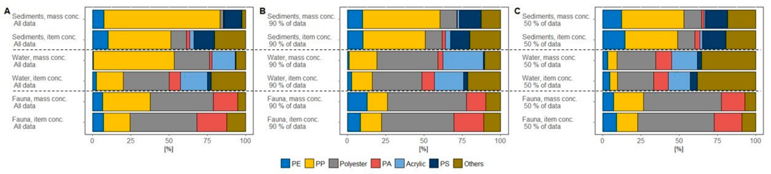
Combining all MPs data from the water, sediments, and fauna, the most abundant polymer was PP, which 35.2% of items and 75.2% of mass was composed of. In at least one of the matrices, PE, PP, polyester, PA, acrylics, or PS accounted for 10% or more of the total number or mass concentration (Figure 3A). For ease of overview, the MPs of other polymers were merged into one group (others) (see Supplementary Materials for details). Comparing the MP mass and number distributions of polymer types revealed no clear correspondence between the mass and number. However, single large particles tended to dominate the polymer distribution in terms of mass, while many small particles tended to dominate the polymer distribution in terms of items. For example, the largest MPs in the sediments (major dimension of 1506 µm) accounted for more than 50% of all the PP mass in this matrix. When removing outliers in terms of the least massive and most massive particles, the mass-based versus number-based polymer composition within each matrix became nearly identical. Figure 3B shows the polymer composition when removing the 5% least massive and the 5% most massive particles, while Figure 3C shows it when removing the 25% least and most massive particles. Regardless of whether outliers were removed, no correspondence between the polymer distributions in water, sediments, and fauna was found.
In the sediments, PP dominated in terms of mass (76%) as well as particle number (41%). The ranking of the polymer composition by mass was PP > PS > PE > other > polyester > acrylic > PA, while the ranking by particle number was PP > other > PE > polyester > PS > acrylic > PA. In the water, polyester dominated the polymeric composition with respect to MP numbers (30%), whereas PP dominated with respect to MP mass (53%). The overall ranking of MP mass in the water was PP > polyester > acrylic > other > PA > PE > PS, while MP numbers ranked polyester > other > PP > acrylic > PA > PE > PS. In the fauna samples, polyester dominated the polymer composition both in terms of mass (41%) and particle number (44%). The overall ranking of MPs in the fauna was polyester > PP > PA > PE > other, while the ranking in terms of mass was polyester > PA > PP > other > PE. The variation of polymeric materials was found to be the lowest in the fauna samples, since only six materials were detected—PE, PP, polyester, PA, epoxy, and a paint particle. The most diverse polymeric composition was found in the sediments, where 16 different material groups were found, followed by the water with 12 material groups. However, it cannot be ruled out that the difference in polymer diversity was related to the analyzed sample size, where more particles were detected for the sediments than for the water and the fauna. Direct comparison of the polymeric composition with other studies is somewhat problematic, as the material composition will depend on the water body, the processes herein, and the sources contributing to the MPs pollution. Nevertheless, the general picture showing that PE, PP, polyester, PA, and, sometimes, acrylic are abundant MPs materials have been reported by many studies of other systems [41,53,54].
3.6. MPs Size Distribution
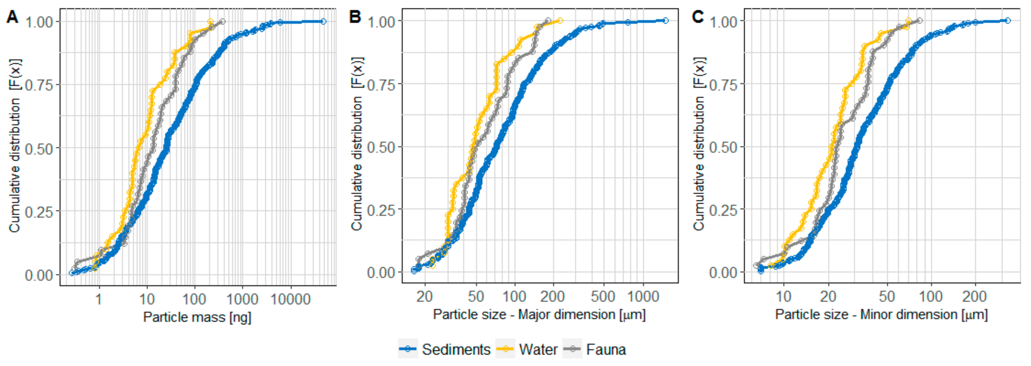
The largest MP particles were found in the sediments. This held true for the mass, volume, and size (Figure 4). The particles tended to be shaped as fragments, i.e., with a length to width ratio below 3. MPs with a ratio above 3 (fibers) constituted 19% of the MPs in the sediments, 23% in the water, and 17% in the fauna. Even sized particles (length to width ratio close to 1) constituted around 7% of all particles. The minor dimension of a particle can be related to the common sieving analysis of soils, where it determines whether a particle can pass a sieving mesh. Comparing the sediment sieving curve to the corresponding calculated pass-through curve of the MPs showed that the size distribution of the MPs in the sediments followed the size distribution of the sediment particles quite closely (see Supplementary Materials for details).
A statistical analysis of the MPs distributions showed that the mass, volume, and size of MPs in the sediments and the water were statistically different (p < 0.05) and that the MPs mass, volume, and size in the water and the fauna were similar (p > 0.50). Comparing the sediments and the fauna showed the same tendency as for the water-sediments comparison; however, the p-value here was 0.0582. An ANOVA analysis and a Tukey test were performed to compare the data, as a Shapiro–Wilk test showed that all data could be considered log-normally distributed.
A large fraction of the particles in the sediments consisted of PP and PE, both polymers with densities lower than freshwater. The largest particle found in the sediments (a PP particle with a minor dimension of 331 µm and major dimension of 1506 µm) would, according to Stokes’ law, have risen towards the water surface with more than a meter per minute, hence it should have floated. Nevertheless, it ended up in the sediments. The mechanisms bringing it and similar particles from the water into the sediments must therefore be different than simple settling processes. From the marine environment, it is well known that buoyant MPs are present in the sediments [45,55] and that processes related to marine snow and biofilm growth can ballast the particles and cause their sedimentation, while also affecting how they are ingested by vertebrates [56,57]. Another possible mechanism is ingestion of MPs by zooplankton or vertebrates and then subsequent egestion as part of their fecal pellets. Such pellets have a higher density than the surrounding water and would act as vectors for the MPs to reach the pond bottom and form part of its sediments [58,59]. Simple hydraulic mixing might also be an explanatory factor for smaller buoyant MPs ending up in the sediments, as stormwater retention ponds are shallow water bodies with high mixing rates, also during dry weather [28]. Small buoyant particles might thus be transported by convective currents at rates higher than their rising velocity and randomly come in contact with the sediment surface, where they might be immobilized due to their hydrophobic properties. The velocity of the convective currents vary with inflow and wind conditions, but can easily be in the cm per second range, which is much higher than the rising velocity of small buoyant MP particles [60].
3.7. Storm Water Ponds as Sinks for MPs
The studied pond retained some, but not all, of the MPs in the ingoing stormwater. The treatment efficiency of the pond with respect to MPs can be roughly estimated from the current study, assuming that the measured water concentration is also the concentration discharged during rain events, that the measured sediment concentration is representative for the accumulated sediments, and by assuming an annual sediment build-up rate. Using the water phase concentrations of Table 1 and the previously calculated inflow to the pond, the MPs discharge from the pond can be estimated to be 1.2 kg year−1. Assuming the pond retains roughly 60 g DM m−3 [28], the corresponding sediment build-up is 16,800 kg DM year−1, corresponding to a retained MPs mass of 6.7 kg year−1. This results in a MPs retainment efficiency of 85%, which is similar to the general treatment efficiency for particulate matter in retention ponds [36]. However, the uncertainty of the assumptions behind these calculations is unknown and probably quite large. This assessment must therefore be seen as a rough first estimate only. Nevertheless, the data shows that stormwater retention ponds are important sinks for microplastics and that such systems play a role in managing diffuse MPs pollution from urban and highway areas.
4. Conclusions
This study showed how a stormwater retention pond designed to detain and treat stormwater runoff from urban areas also acts as a sink for MPs from the runoff. A rough first estimate showed that the retention of MPs in the pond was probably similar to the retention of particulate material in general and that MPs concentrations in treated stormwater were somewhat comparable to those of treated wastewater from nutrient-removing treatment plants. The MPs accumulated to quite high concentrations in the sediments, but also in vertebrates, the latter to a level nearly as high as in the sediments. The observation that MPs accumulated to quite high concentrations in the vertebrates of the ponds is a cause for concern as to whether this can have adverse impacts on the pond ecosystems. From this investigation, it seems clear that retention ponds in general do have a role to play in managing MPs pollution in urban runoff. It does, however, also show that the quantification of the overall retention was somewhat tenuous, as was the determination of concentrations, especially in the sediments and fauna, calling for improvements of the analytical procedures and further quantitative studies.
Supplementary Materials
The following are available online at https://www.mdpi.com/2073-4441/11/7/1466/s1.
Author Contributions
K.B.O. carried out the experiments, interpreted the results, and wrote the initial draft. D.A.S. contributed to the sampling and sample preparation. N.v.A. conducted the µFTIR scanning’s and contributed to interpreting the data. J.V. developed the MPhunter software and supervised the project. All authors contributed to the final manuscript.
Funding
This research received no external funding.
Conflicts of Interest
The authors declare no conflict of interest.
References
- Andrady, A.L. Microplastics in the Marine Environment. Mar. Pollut. Bull. 2011, 62, 1596–1605. [Google Scholar] [CrossRef] [PubMed]
- Rhodes, C.J. Plastic Pollution and Potential Solutions. Sci. Prog. 2018, 101, 207–260. [Google Scholar] [CrossRef] [PubMed]
- Dris, R.; Gasperi, J.; Rocher, V.; Saad, M.; Renault, N.; Tassin, B. Microplastic Contamination in an Urban Area: A Case Study in Greater Paris. Environ. Chem. 2015, 12, 592–599. [Google Scholar] [CrossRef]
- Fahrenfeld, N.L.; Arbuckle-Keil, G.; Naderi Beni, N.; Bartelt-Hunt, S.L. Source Tracking Microplastics in the Freshwater Environment. Trends Anal. Chem. 2019, 112, 248–254. [Google Scholar] [CrossRef]
- Bordós, G.; Urbányi, B.; Micsinai, A.; Kriszt, B.; Palotai, Z.; Szabó, I.; Hantosi, Z.; Szoboszlay, S. Identification of Microplastics in Fish Ponds and Natural Freshwater Environments of the Carpathian Basin, Europe. Chemosphere 2019, 216, 110–116. [Google Scholar] [CrossRef] [PubMed]
- Luo, W.; Su, L.; Craig, N.J.; Du, F.; Wu, C.; Shi, H. Comparison of Microplastic Pollution in Different Water Bodies from Urban Creeks to Coastal Waters. Environ. Pollut. 2019, 246, 174–182. [Google Scholar] [CrossRef]
- Kataoka, T.; Nihei, Y.; Kudou, K.; Hinata, H. Assessment of the Sources and Inflow Processes of Microplastics in the River Environments of Japan. Environ. Pollut. 2019, 244, 958–965. [Google Scholar] [CrossRef]
- Ballent, A.; Corcoran, P.L.; Madden, O.; Helm, P.A.; Longstaffe, F.J. Sources and Sinks of Microplastics in Canadian Lake Ontario Nearshore, Tributary and Beach Sediments. Mar. Pollut. Bull. 2016, 110, 383–395. [Google Scholar] [CrossRef]
- Mintenig, S.M.; Int-Veen, I.; Löder, M.G.J.; Primpke, S.; Gerdts, G. Identification of Microplastic in Effluents of Waste Water Treatment Plants Using Focal Plane Array-Based Micro-Fourier-Transform Infrared Imaging. Water Res. 2017, 108, 365–372. [Google Scholar] [CrossRef]
- Talvitie, J.; Mikola, A.; Setälä, O.; Heinonen, M.; Koistinen, A. How Well Is Microlitter Purified from Wastewater?—A Detailed Study on the Stepwise Removal of Microlitter in a Tertiary Level Wastewater Treatment Plant. Water Res. 2017, 109, 164–172. [Google Scholar] [CrossRef]
- Simon, M.; van Alst, N.; Vollertsen, J. Quantification of Microplastic Mass and Removal Rates at Wastewater Treatment Plants Applying Focal Plane Array (FPA)-Based Fourier Transform Infrared (FT-IR) Imaging. Water Res. 2018, 142, 1–9. [Google Scholar] [CrossRef] [PubMed]
- Lasee, S.; Mauricio, J.; Thompson, W.A.; Karnjanapiboonwong, A.; Kasumba, J.; Subbiah, S.; Morse, A.; Anderson, T.A. Microplastics in a Freshwater Environment Receiving Treated Wastewater Effluent: Microplastics in Urban Surface Water. Integr. Environ. Assess. Manag. 2017, 13, 528–532. [Google Scholar] [CrossRef] [PubMed]
- Horton, A.A.; Walton, A.; Spurgeon, D.J.; Lahive, E.; Svendsen, C. Microplastics in Freshwater and Terrestrial Environments: Evaluating the Current Understanding to Identify the Knowledge Gaps and Future Research Priorities. Sci. Total Environ. 2017, 586, 127–141. [Google Scholar] [CrossRef] [PubMed]
- Song, Y.K.; Hong, S.H.; Jang, M.; Han, G.M.; Rani, M.; Lee, J.; Shim, W.J. A Comparison of Microscopic and Spectroscopic Identification Methods for Analysis of Microplastics in Environmental Samples. Mar. Pollut. Bull. 2015, 93, 202–209. [Google Scholar] [CrossRef]
- Lusher, A.L.; Welden, N.A.; Sobral, P.; Cole, M. Sampling, Isolating and Identifying Microplastics Ingested by Fish and Invertebrates. Anal. Methods 2017, 1346–1360. [Google Scholar] [CrossRef]
- Miller, M.E.; Kroon, F.J.; Motti, C.A. Recovering Microplastics from Marine Samples: A Review of Current Practices. Mar. Pollut. Bull. 2017, 123, 6–18. [Google Scholar] [CrossRef]
- Shim, W.J.; Hongab, S.H.; Eo, S.E. Identification Methods in Microplastic Analysis: A Review. Anal. Methods 2017, 1384–1391. [Google Scholar] [CrossRef]
- Primpke, S.; Lorenz, C.; Rascher-Friesenhausen, R.; Gerdts, G. An Automated Approach for Microplastics Analysis Using Focal Plane Array (FPA) FTIR Microscopy and Image Analysis. Anal. Methods 2017, 9, 1499–1511. [Google Scholar] [CrossRef]
- Browne, M.A.; Crump, P.; Niven, S.J.; Teuten, E.; Tonkin, A.; Galloway, T.; Thompson, R. Accumulation of Microplastic on Shorelines Woldwide: Sources and Sinks—Environmental Science & Technology (ACS Publications). Environ. Sci. Technol. 2011, 9175–9179. [Google Scholar] [CrossRef]
- Filella, M. Questions of Size and Numbers in Environmental Research on Microplastics: Methodological and Conceptual Aspects. Environ. Chem. 2015, 12, 527–538. [Google Scholar] [CrossRef]
- Liu, F.; Olesen, K.B.; Borregaard, A.R.; Vollertsen, J. Microplastics in Urban and Highway Stormwater Retention Ponds. Sci. Total Environ. 2019, 671, 992–1000. [Google Scholar] [CrossRef]
- Steele, M.K.; Heffernan, J.B. Morphological Characteristics of Urban Water Bodies: Mechanisms of Change and Implications for Ecosystem Function. Ecol. Appl. 2014, 24, 1070–1084. [Google Scholar] [CrossRef] [PubMed]
- Williams, C.J.; Frost, P.C.; Xenopoulos, M.A. Beyond Best Management Practices: Pelagic Biogeochemical Dynamics in Urban Stormwater Ponds. Ecol. Appl. 2013, 23, 1384–1395. [Google Scholar] [CrossRef] [PubMed]
- Bishop, C.A.; Struger, J.; Barton, D.R.; Shirose, L.J.; Dunn, L.; Lang, A.L.; Shepherd, D. Contamination and Wildlife Communities in Stormwater Detention Ponds in Guelph and the Greater Toronto Area, Ontario, 1997 and 1998. Part I—Wildlife Communities. Water Qual. Res. J. 2000, 35, 399–435. [Google Scholar] [CrossRef]
- Stephansen, D.A.; Nielsen, A.H.; Hvitved-Jacobsen, T.; Pedersen, M.L.; Vollertsen, J. Invertebrates in Stormwater Wet Detention Ponds—Sediment Accumulation and Bioaccumulation of Heavy Metals Have No Effect on Biodiversity and Community Structure. Sci. Total Environ. 2016, 566–567, 1579–1587. [Google Scholar] [CrossRef] [PubMed]
- Thorndahl, S.; Johansen, C.; Schaarup-Jensen, K. Assessment of Runoff Contributing Catchment Areas in Rainfall Runoff Modelling. Water Sci. Technol. 2006, 54, 49–56. [Google Scholar] [CrossRef] [PubMed]
- Brezonik, P.L.; Stadelmann, T.H. Analysis and Predictive Models of Stormwater Runoff Volumes, Loads, and Pollutant Concentrations from Watersheds in the Twin Cities Metropolitan Area, Minnesota, USA. Water Res. 2002, 36, 1743–1757. [Google Scholar] [CrossRef]
- Hvitved-Jacobsen, T.; Vollertsen, J.; Nielsen, A.H. Fundamentals of Urban Highway Stormwater Pollution. In Urban and Highway Stormwater Pollution: Concepts and Engineering; Taylor & Francis: Boca Raton, FL, USA, 2010; pp. 1–20. [Google Scholar]
- Vollertsen, J.; Hvitved-Jacobsen, T.; Nielsen, H.; Gabriel, S. Våde Bassiner til Rensning af Separat Regnvand—Baggrundsrapport; Teknologisk Institute: Taastrup, Denmark, 2012; p. 71. [Google Scholar]
- Cole, M.; Webb, H.; Lindeque, P.K.; Fileman, E.S.; Halsband, C.; Galloway, T.S. Isolation of Microplastics in Biota-Rich Seawater Samples and Marine Organisms. Sci. Rep. 2014, 4, 1–8. [Google Scholar] [CrossRef] [PubMed]
- Foekema, E.M.; De Gruijter, C.; Mergia, M.T.; Van Franeker, J.A.; Murk, A.J.; Koelmans, A.A. Plastic in North Sea Fish. Environ. Sci. Technol. 2013, 47, 8818–8824. [Google Scholar] [CrossRef] [PubMed]
- Dehaut, A.; Cassone, A.L.; Frère, L.; Hermabessiere, L.; Himber, C.; Rinnert, E.; Rivière, G.; Lambert, C.; Soudant, P.; Huvet, A.; et al. Microplastics in Seafood: Benchmark Protocol for Their Extraction and Characterization. Environ. Pollut. 2016, 215, 223–233. [Google Scholar] [CrossRef]
- WHO. Determination of Airborne Fibre Number Concentrations: A Recommended Method, by Phase-Contrast Optical Microscopy (Membrane Filter Method); WHO: Geneve, Switzerland, 1997. [Google Scholar]
- Rice, E.W.; Baird, R.B.; Eaton, A.D.; Clesceri, L.S. Solids. In Standard Methods for the Examination of Water and Wastewater; American Public Health Association, American Water Works Association, Water Environment Federation: Washington, DC, USA, 2012. [Google Scholar]
- Jones, J.R.; Obrecht, D.V.; Perkins, B.D.; Knowlton, M.F.; Thorpe, A.P.; Watanabe, S.; Bacon, R.R. Nutrients, Seston, and Transparency of Missouri Reservoirs and Oxbow Lakes: An Analysis of Regional Limnology. Lake Reserv. Manag. 2008, 24, 155–180. [Google Scholar] [CrossRef]
- Clary, J.; Jones, J. International Stormwater BMP Database 2016 SUMMARY STATISTICS; Water Environ. Reuse Found. 2017. Available online:www.bmpdatabase.org (accessed on 1 March 2019).
- Blaszczak, J.R.; Steele, M.K.; Badgley, B.D.; Heffernan, J.B.; Hobbie, S.E.; Morse, J.L.; Rivers, E.N.; Hall, S.J.; Neill, C.; Pataki, D.E.; et al. Sediment Chemistry of Urban Stormwater Ponds and Controls on Denitrification. Ecosphere 2018, 9. [Google Scholar] [CrossRef]
- Hurley, R.R.; Lusher, A.L.; Olsen, M.; Nizzetto, L. Validation of a Method for Extracting Microplastics from Complex, Organic-Rich, Environmental Matrices. Environ. Sci. Technol. 2018, 52, 7409–7417. [Google Scholar] [CrossRef] [PubMed] [Green Version]
- Eisentraut, P.; Dümichen, E.; Ruhl, A.S.; Jekel, M.; Albrecht, M.; Gehde, M.; Braun, U. Two Birds with One Stone—Fast and Simultaneous Analysis of Microplastics: Microparticles Derived from Thermoplastics and Tire Wear. Environ. Sci. Technol. 2018, 5, 608–613. [Google Scholar] [CrossRef]
- Zhu, J.; Zhang, Q.; LI, Y.; Tan, S.; Kang, Z.; Yu, X.; Lan, W.; Cai, L.; Wang, J.; Shi, H. Microplastic Pollution in the Maowei Sea, a Typical Mariculture Bay of China. Sci. Total Environ. 2019, 62–68. [Google Scholar] [CrossRef] [PubMed]
- Rodrigues, M.O.; Abrantes, N.; Gonçalves, F.J.M.; Nogueira, H.; Marques, J.C.; Gonçalves, A.M.M. Spatial and Temporal Distribution of Microplastics in Water and Sediments of a Freshwater System (Antuã River, Portugal). Sci. Total Environ. 2018, 633, 1549–1559. [Google Scholar] [CrossRef] [PubMed]
- Löder, M.G.J.; Imhof, H.K.; Ladehoff, M.; Löschel, L.A.; Lorenz, C.; Mintenig, S.; Piehl, S.; Primpke, S.; Schrank, I.; Laforsch, C.; et al. Enzymatic Purification of Microplastics in Environmental Samples. Environ. Sci. Technol. 2017, 51, 14283–14292. [Google Scholar] [CrossRef]
- Tibbetts, J.; Krause, S.; Lynch, I.; Smith, G.H.S. Abundance, Distribution, and Drivers of Microplastic Contamination in Urban River Environments. Water (Switz.) 2018, 10, 1597. [Google Scholar] [CrossRef]
- Klein, S.; Worch, E.; Knepper, T.P. Occurrence and Spatial Distribution of Microplastics in River Shore Sediments of the Rhine-Main Area in Germany. Environ. Sci. Technol. 2015, 49, 6070–6076. [Google Scholar] [CrossRef]
- Vianello, A.; Boldrin, A.; Guerriero, P.; Moschino, V.; Rella, R.; Sturaro, A.; Da Ros, L. Microplastic Particles in Sediments of Lagoon of Venice, Italy: First Observations on Occurrence, Spatial Patterns and Identification. Estuar. Coast. Shelf Sci. 2013, 130, 54–61. [Google Scholar] [CrossRef]
- Møskeland, T.; Laugesen, J.; Jensen, T.; Knutsen, H.; Arp, H.P.; Lilleeng, Ø.; Pettersen, A. Microplastics in Sediments on the Norwegian Continental Shelf; 2018-0050, Rev. 01; Miljødirektoratet: Trondheim, Norway, 2018. [Google Scholar]
- Jabeen, K.; Su, L.; Li, J.; Yang, D.; Tong, C.; Mu, J.; Shi, H. Microplastics and Mesoplastics in Fish from Coastal and Fresh Waters of China. Environ. Pollut. 2017, 221, 141–149. [Google Scholar] [CrossRef] [PubMed]
- Nelms, S.E.; Galloway, T.S.; Godley, B.J.; Jarvis, D.S.; Lindeque, P.K. Investigating Microplastic Trophic Transfer in Marine Top Predators. Environ. Pollut. 2018, 238, 999–1007. [Google Scholar] [CrossRef] [PubMed]
- Rochman, C.M.; Tahir, A.; Williams, S.L.; Baxa, D.V.; Lam, R.; Miller, J.T.; Teh, F.-C.; Werorilangi, S.; Teh, S.J. Anthropogenic Debris in Seafood: Plastic Debris and Fibers from Textiles in Fish and Bivalves Sold for Human Consumption. Sci. Rep. 2015, 5, 1–10. [Google Scholar] [CrossRef] [PubMed]
- Lusher, A.L.; O’Donnell, C.; Officer, R.; O’Connor, I. Microplastic Interactions with North Atlantic Mesopelagic Fish. ICES J. Mar. Sci. 2015, 69, 1–11. [Google Scholar] [CrossRef]
- Yuan, W.; Liu, X.; Wang, W.; Di, M.; Wang, J. Microplastic Abundance, Distribution and Composition in Water, Sediments, and Wild Fish from Poyang Lake, China. Ecotoxicol. Environ. Saf. 2019, 170, 180–187. [Google Scholar] [CrossRef] [PubMed]
- Herrera, A.; Ŝtindlová, A.; Martínez, I.; Rapp, J.; Romero-Kutzner, V.; Samper, M.D.; Montoto, T.; Aguiar-González, B.; Packard, T.; Gómez, M. Microplastic Ingestion by Atlantic Chub Mackerel (Scomber Colias) in the Canary Islands Coast. Mar. Pollut. Bull. 2019, 139, 127–135. [Google Scholar] [CrossRef]
- Kanhai, L.D.K.; Officer, R.; Lyashevska, O.; Thompson, R.C.; O’Connor, I. Microplastic Abundance, Distribution and Composition along a Latitudinal Gradient in the Atlantic Ocean. Mar. Pollut. Bull. 2017, 115, 307–314. [Google Scholar] [CrossRef]
- Erni-cassola, G.; Zadjelovic, V.; Gibson, M.I.; Christie-oleza, J.A. Distribution of Plastic Polymer Types in the Marine Environment; A Meta- Analysis. J. Hazard. Mater. 2019, 369, 691–698. [Google Scholar] [CrossRef]
- Peng, G.; Zhu, B.; Yang, D.; Su, L.; Shi, H.; Li, D. Microplastics in Sediments of the Changjiang Estuary, China. Environ. Pollut. 2017, 225, 283–290. [Google Scholar] [CrossRef]
- Kooi, M.; van Nes, E.H.; Scheffer, M.; Koelmans, A.A. Ups and Downs in the Ocean: Effects of Biofouling on Vertical Transport of Microplastics. Environ. Sci. Technol. 2017, 51, 7963–7971. [Google Scholar] [CrossRef] [Green Version]
- Porter, A.; Lyons, B.P.; Galloway, T.S.; Lewis, C. Role of Marine Snows in Microplastic Fate and Bioavailability. Environ. Sci. Technol. 2018, 52, 7111–7119. [Google Scholar] [CrossRef] [PubMed]
- Cole, M.; Lindeque, P.K.; Fileman, E.; Clark, J.; Lewis, C.; Halsband, C.; Galloway, T.S. Microplastics Alter the Properties and Sinking Rates of Zooplankton Faecal Pellets. Environ. Sci. Technol. 2016, 50, 3239–3246. [Google Scholar] [CrossRef] [PubMed] [Green Version]
- Belcher, A.; Tarling, G.A.; Manno, C.; Atkinson, A.; Ward, P.; Skaret, G.; Fielding, S.; Henson, S.A.; Sanders, R. The Potential Role of Antarctic Krill Faecal Pellets in Efficient Carbon Export at the Marginal Ice Zone of the South Orkney Islands in Spring. Polar Biol. 2017, 40, 2001–2013. [Google Scholar] [CrossRef]
- Bentzen, T.R.; Larsen, T.; Rasmussen, M.R. Wind Effects on Retention Time in Highway Ponds. Water Sci. Technol. 2008, 57, 1713–1720. [Google Scholar] [CrossRef] [PubMed]
Figure 1.
The sampled pond, its catchment, and the locations at which samples were collected. The sediments were sampled in the area marked with a dotted square, the water was sampled in the area marked with a dotted circle, and the fish were caught in the area marked with a dotted line. The blue lines show the inlets where stormwater is discharged into the pond and the red dotted line shows the outlet pipe of the pond.

Figure 2.
Protocol for treatment and analysis of samples.

Figure 3.
Polymeric composition of sediments, water and fauna. (A) All data. (B) The 5% least and most massive microplastic particles (MPs) excluded. (C) The 25% least and most massive MPs excluded.
Figure 3.
Polymeric composition of sediments, water and fauna. (A) All data. (B) The 5% least and most massive microplastic particles (MPs) excluded. (C) The 25% least and most massive MPs excluded.

Figure 4.
Cumulative distribution of the detected MP particles with respect to (A) summarized mass in percentage, (B) particle size (minor dimension) of sediment MP particles, and (C) particle size (minor dimension) of water and fauna MP particles.
Figure 4.
Cumulative distribution of the detected MP particles with respect to (A) summarized mass in percentage, (B) particle size (minor dimension) of sediment MP particles, and (C) particle size (minor dimension) of water and fauna MP particles.


Table 1.
MP mass and MP particle number concentrations in the stormwater retention pond. Particle mass and number concentrations are not corrected for blank values.
Table 1.
MP mass and MP particle number concentrations in the stormwater retention pond. Particle mass and number concentrations are not corrected for blank values.
| Particle Concentration | Blank | Unit * | Mass Concentration | Blank | Unit * | |
|---|---|---|---|---|---|---|
| Sediments | 9.5 × 10⁵ | 5 × 10³ | item (kg DW)−1 | 401.5 | 0.4 | mg (kg DW)−1 |
| Water | 2.7 × 10⁵ | 1 × 10⁴ | item m−3 | 4.2 | 0.8 | mg m−3 |
| Fauna | 3.4 × 10⁵ | 5 × 10⁴ | item (kg DW)−1 | 12.9 | 3.9 | mg (kg DW)−1 |
* DW, dry weight of sediments or fauna.
© 2019 by the authors. Licensee MDPI, Basel, Switzerland. This article is an open access article distributed under the terms and conditions of the Creative Commons Attribution (CC BY) license (http://creativecommons.org/licenses/by/4.0/).
Share and Cite
MDPI and ACS Style
Olesen, K.B.; Stephansen, D.A.; van Alst, N.; Vollertsen, J. Microplastics in a Stormwater Pond. Water 2019, 11, 1466. https://doi.org/10.3390/w11071466
AMA Style
Olesen KB, Stephansen DA, van Alst N, Vollertsen J. Microplastics in a Stormwater Pond. Water. 2019; 11(7):1466. https://doi.org/10.3390/w11071466
Chicago/Turabian StyleOlesen, Kristina Borg, Diana A. Stephansen, Nikki van Alst, and Jes Vollertsen. 2019. "Microplastics in a Stormwater Pond" Water 11, no. 7: 1466. https://doi.org/10.3390/w11071466
Note that from the first issue of 2016, this journal uses article numbers instead of page numbers. See further details here.