Hydrogeological Bayesian Hypothesis Testing through Trans-Dimensional Sampling of a Stochastic Water Balance Model

Abstract

Conceptual uncertainty is considered one of the major sources of uncertainty in groundwater flow modelling. In this regard, hypothesis testing is essential to increase system understanding by refuting alternative conceptual models. Often a stepwise approach, with respect to complexity, is promoted but hypothesis testing of simple groundwater models is rarely applied. We present an approach to model-based Bayesian hypothesis testing in a simple groundwater balance model, which involves optimization of a model in function of both parameter values and conceptual model through trans-dimensional sampling. We apply the methodology to the Wildman River area, Northern Territory, Australia, where we set up 32 different conceptual models. A factorial approach to conceptual model development allows for direct attribution of differences in performance to individual uncertain components of the conceptual model. The method provides a screening tool for prioritizing research efforts while also giving more confidence to the predicted water balance compared to a deterministic water balance solution. We show that the testing of alternative conceptual models can be done efficiently with a simple additive and linear groundwater balance model and is best done relatively early in the groundwater modelling workflow.

1. Introduction

The conceptualization of a groundwater flow problem is considered one of the major sources of uncertainty in groundwater flow modelling [1,2]. Conceptual uncertainty stems from the fact that the available data more often than not will fit more than one conceptual understanding [3]. When dealing with conceptual uncertainty, hypothesis testing is essential to increase system understanding by refuting alternative conceptual models [4].

The question we ask of the hypothesis testing exercise is framed by the model development approach. In practice, individual conceptual hypotheses cannot be tested through model-based hypothesis testing; only collections of hypotheses can be tested [5,6]. That is, if a hypothesis cannot be falsified in a model, it is only conditionally validated given the assumptions in other parts of the model. The challenge is to develop alternative models so that differences in performance can be attributed to individual hypotheses. For exploratory purposes, model development should aim at maximizing the difference between alternative models in order to gain the most information from a potential model rejection [7,8].

One branch of hypothesis testing is based on the Bayesian probability theory. In Bayesian hypothesis testing, a prior belief about the suitability of a conceptual model is updated to a posterior belief by evaluating the model performance against data. The performance of alternative models are then compared in order to quantitatively rank and potentially reject hypotheses based on the so-called Bayes factor [9,10]. Fields of application in hydrogeology include groundwater modelling [11,12], hydrogeophysics [13,14] and solute transport modelling [15,16]. In many applications, the data is not sufficient to allow for discrimination between the models, in which case Bayesian model averaging is often applied where model predictions are weighed according to their performance against data [17].

In hydrogeology, conceptual models are often tested in mathematical models (e.g., [18,19]). Since a model comprises the description of a system as a whole, all assumptions and the interaction of assumptions are tested at once. Also, data that does not directly relate to the conceptually uncertain feature can be integrated because of the holistic testing of the system.

A stepwise approach in regards to the complexity of groundwater flow modelling and hypothesis testing is often promoted [20,21]. In this paper the simplicity of a model is defined in terms of setup and run-time. In a stepwise approach, complexity is gradually built up, and involves testing the models in each step to better understand the relative importance of various assumptions. This is opposed to starting with a complex model where all known processes and structural aspects are incorporated “because they exist, not because they matter” [20].

Although there seems to be a consensus that testing simple models is advantageous, most model-based hypothesis testing in hydrogeology happens in complex models. We argue that there is a need to also test models as early as possible with models being as simple as possible for at least four reasons. First, simple models can offer insight into system understanding that can be obscured in more complex models [22,23]. Second, testing models early in the workflow enables identification of important sources of uncertainty and knowledge gaps to help prioritize research efforts, including data collection [24]. Third, pragmatic constraints on time and budget limit the number of models that can be tested and fewer models are tested when they are more complex [25]. Finally, rigorous model testing identifies conceptual surprises early in the research effort, rather than detecting them after modelling is completed. A stepwise approach to groundwater modelling is especially important when the multi-model approach is adopted; this is still mainly an academic exercise since developing several conceptual models rather than a single one is a time-consuming task.

One of the most widely applied and simplest approaches to represent a groundwater system is through an additive groundwater system water balance [26,27]. Water balances are systematic records of the water fluxes going into and out of a groundwater system, and how these fluxes affect the stored volumes of water. The estimation of uncertainties in water balance components is the topic of several studies [28,29,30], but conceptualization issues are rarely considered. By applying different conceptualizations, the number of parameters describing the water balance is variable. A trans-dimensional [31] inverse problem is one where the dimension of the parameter space, not just values of the parameters, is a variable to be solved for. Within the geosciences, trans-dimensional sampling is most often applied in geophysics (e.g., [32]), but has gained ground in hydrology in recent years [33,34,35]. In this paper we apply trans-dimensional sampling to a stochastic water balance in order to test conceptually uncertain components in the water balance problem.

The aim of this study is to (1) develop a model development framework to test alternative conceptual models in a Bayesian framework, (2) apply it to a simple groundwater balance model and (3) evaluate if there is sufficient information in the water balance to gain insight on the conceptualization of a groundwater system. We apply this methodology to the Wildman River area in the Northern Territory, Australia.

2. Materials and Methods

A simplified representation of the applied methodology is illustrated in Figure 1. In the stochastic water balance, different components, represented by different coloured circles, are included or excluded in the water balance equation in order to represent conceptual uncertainty. In each parameter realization, the magnitude of the components is varied in order to represent aleatory uncertainty (i.e., uncertainty that can be modelled stochastically), represented by the size of the circle in Figure 1a. The likelihood of each of these parameter and model realizations is based on the error of the water balance and a Metropolis–Hastings sampler [36,37] is applied over these likelihoods (Figure 1b) in order to estimate the probability of the different plausible models. The more likely a model is, the more often the sampling algorithm will visit the model. The posterior probability of a model is the number of accepted visits that is based on an acceptance probability. An inter-comparison of the posterior model probabilities reveals whether some models are preferred over others based on predefined threshold values of the Bayes factor. More details about the workflow illustrated in Figure 1 will be provided in Section 2.4.

In the following section, a detailed description of the methodology is presented. First, we propose an alternative model development methodology, and introduce the Bayesian inference and interpretation methods. The methodology described in these sections are entirely generic and therefore applicable to any type of model. Last, we describe the setup of the groundwater balance that facilitates effortless evaluation of numerous model realizations.

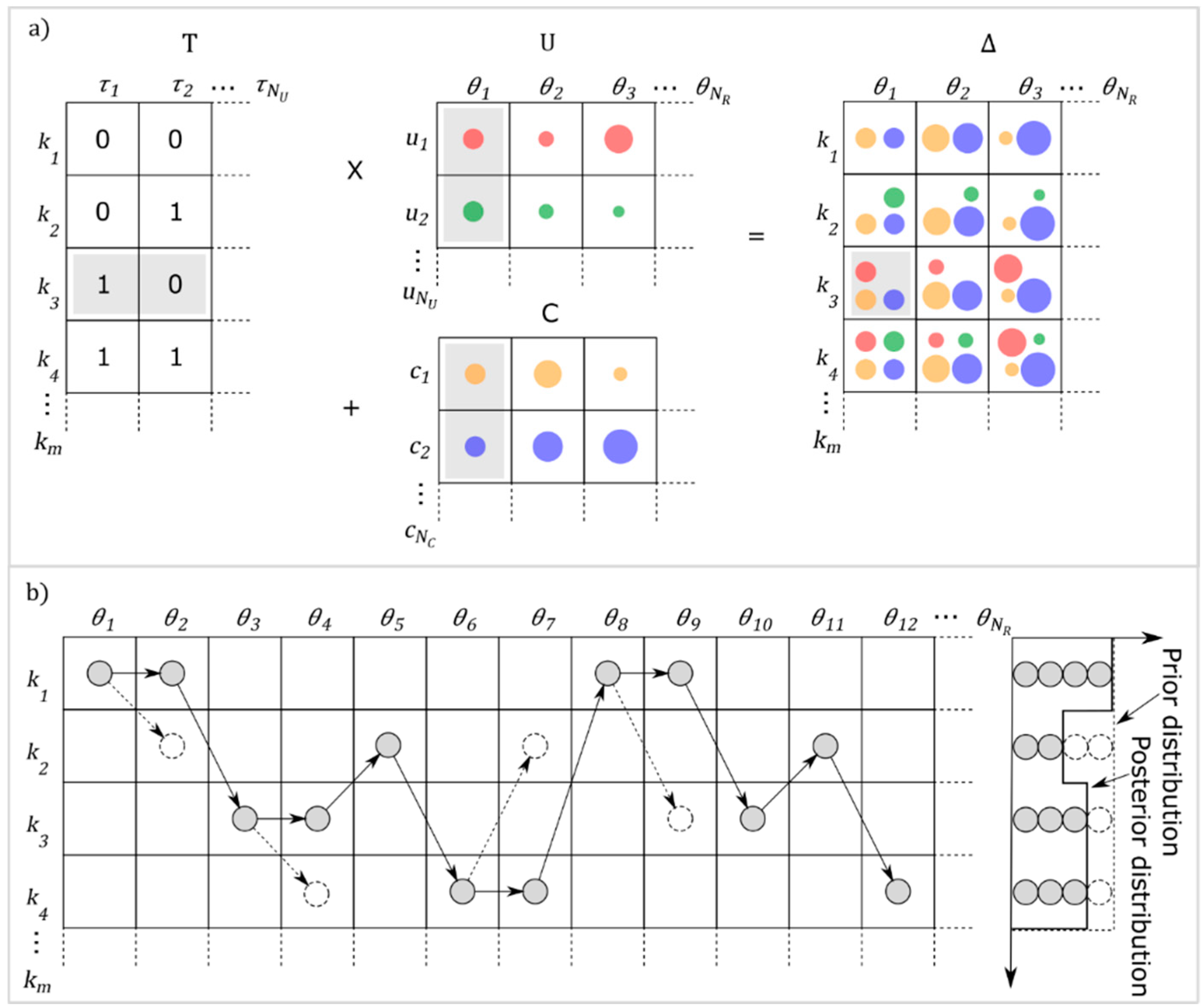
2.1. Model Development Method

Conceptual models can generally be decomposed into a collection of hypotheses that describe the conceptual physical structure and the conceptual process structure [1]. Note that the term conceptual model comprises a collection of hypotheses, while the term hypothesis concerns individual uncertain components in the conceptual model. More often than not, uncertain components will exist in the conceptual model, either to do with the geometry (e.g., hydrostratigraphy) or processes (i.e., boundary conditions) in the groundwater system. We suggest defining hypotheses for each conceptually uncertain component in the conceptual model in the following manner:

• H₀: The process/geometry does not matter for the prediction of interest.
• H_A: The process/geometry matters for the prediction of interest.

In the null hypothesis (H₀) the uncertain component is excluded, while the alternative hypothesis (H_A) will include the uncertain component. Although we apply a Bayesian hypothesis testing framework, we borrow the null and alternative hypothesis terminology from null hypothesis significance testing to illustrate that the two hypotheses are mutually exclusive. This framework ensures models are mutually exclusive, so that the probability of the null hypothesis and the alternative hypothesis for a single uncertain component adds up to one. Making a statement about whether the conceptually uncertain component matters for the prediction of interest rather than whether it is present or not, places emphasis on the objective of the modelling exercise and makes the hypotheses easier to disprove.

In a mathematical model, we can add an extra parameter to represent the conceptual uncertainty. We can turn an uncertain conceptual component on or off in function of ${\tau }_h$ with $h\in \left\{1,\dots ,m\right\}$ that takes a value of either 0 or 1. Here ${\tau }_h=0$ represents the null hypothesis and ${\tau }_h=1$ represents the alternative hypothesis. For the number of uncertain components, $N_U$, the number of possible combinations of the null and the alternative hypotheses is $m=2^{N_U}$. All possible models can be defined in matrix T, where each row represents an individual conceptual model, $k_j$ with $j\in \left\{1,\dots ,m\right\}$ (Figure 1a):

$$\mathrm{T}=\left[\begin{array}{cccc}{\tau }_{1,1}& {\tau }_{1,2}& \cdots & {\tau }_{1,N_U}\\ {\tau }_{2,1}& {\tau }_{2,2}& \cdots & {\tau }_{2,N_U}\\ ⋮& ⋮& \ddots & ⋮\\ {\tau }_{m,1}& {\tau }_{m,2}& \dots & {\tau }_{m,N_U}\end{array}\right]\begin{array}{c}{k}_1\\ k_2\\ ⋮\\ k_m\end{array}$$

(1)

By developing alternative models with a factorial design [39] of uncertain model components, the difference in model performance can be attributed to individual uncertain model components.

In hydrogeology, similar approaches have previously been presented (e.g., [15,40,41]). This factorial approach is in contrast to approaches where alternative model development hypotheses are grouped in alternative models [42,43,44], thus limiting the information that can be gained from the modelling exercise. Hierarchical Bayesian model averaging (HBMA) (e.g., [45,46]), presents a similar approach that also aims at separating and quantifying the contribution of uncertain model components to prioritize and provide an understanding of a conceptual model. The main difference between the model building approach in HBMA and the one presented here, is that in HBMA the hypotheses are not necessarily mutually exclusive.

2.2. Bayesian Inference Framework

The goal of the Bayesian inference is to compute posterior probabilities for parameters and hypotheses based on data. When the dimension of the parameter vector is one of the unknowns, the joint posterior probability, $p\left(k,{\theta }_k|Y\right)$ of the model indicator $k$ and a parameter vector, ${\theta }_k$ given the data, $Y$, becomes the basis of the inference, and the problem can be categorized as trans-dimensional. The inference starts from a prior probability of models, $p\left(k\right)$, and a prior probability of parameters $p({\theta }_k|k)$, for each model, $k$. The prior is linked to the posterior through a likelihood function, $p\left(Y|k,{\theta }_k\right)$:

$$p\left(k,{\theta }_k|Y\right)=p\left(Y|k,{\theta }_k\right)p({\theta }_k|k)$$

(2)

The likelihood function describes the probability of the observed data given the model. To approximate the posterior probability, we apply Markov chain Monte Carlo simulation where each iteration consists of moving from the current parameter vector ${\theta }^p$ to the proposed parameter vector ${\theta }^q$ and from the current model $k$ to the proposed model, $k^{\prime }$ (Figure 1b). If the proposal distribution is symmetric, each iteration step can be accepted with an acceptance probability, $\alpha$, of [47]:

$$\alpha =\min \left\{1,\frac{p\left(Y|{\theta }^q,k^{\prime }\right)p\left(k^{\prime }\right)}{p\left(Y|{\theta }^p,k\right)p\left(k\right)}\right\}$$

(3)

In practice, models are accepted if a uniform random number between 0 and 1 is lower than the acceptance probability, $\alpha$. If the acceptance probability is lower than this random number between 0 and 1, the proposed model position (${\theta }^q, k^{\prime })$ is rejected and the algorithm stays at position $({\theta }^p, k)$.

2.3. Interpretation

The Bayesian hypothesis testing problem involves interpretation of the marginal evidence for each model, $p\left(Y,k\right)$. The marginal evidence is obtained by integrating the posterior over all plausible model parameters and describes how well the model explains data taking all plausible parameter combinations into account.

For pairwise comparison of the evidence provided by data for models, the Bayes factor can be calculated. When the probabilities are converted to an odds scale (odds = probability/(1 − probability), the Bayes factor is defined as [9]:

$$B_{1,2}=\frac{p\left(k_1|Y\right)p\left(k_2\right)}{p\left(k_2|Y\right)p\left(k_1\right)}$$

(4)

where the two indices, 1 and 2, are used here as a simple example to indicate two mutually exclusive models. When prior probabilities are uniform, the Bayes factor is equal to the ratio of posterior probabilities. To ease interpretation, Kass and Raftery applied descriptions of the evidence provided for intervals of the Bayesian factor [9] (

Table 1. Interpretation of level of support for model $k_1$ or $k_2$ from Bayes factors as defined in Equation (4), with $k_1$ in the numerator and $k_2$ in the denominator. When the probability of $k_1$ and $k_2$ is 1, the ranges of Bayes factor correspond to the probabilities in the “Probabilities” column.

Bayes Factor	Probabilities	Description
<0.005	<0.075	Decisive support for k2
0.005–0.05	0.075–0.182	Strong support for k2
0.05–0.3	0.182–0.366	Substantial support for k2
0.3–3	0.366–0.634	Inconclusive, no support for either k1 or k2
3–20	0.634–0.818	Substantial support for k1
20–150	0.818–0.925	Strong support for k1
>150	>0.925	Decisive support for k1

). A Bayes factor below 1 shows support for the model in the denominator ($k_2$). These thresholds can be used as a guideline for decisions about model selection or rejection, however the interpretation may depend on context.

2.4. Water Balance Model

The additive groundwater balance approach is based on the conservation of mass principle subtracting the water flowing out of the aquifer from the water flowing into the aquifer over a specified time period. We use positive numbers for water going into the aquifer and negative numbers for water going out of the aquifer. In this study we will independently identify the contribution of each component in the water balance, so that no component will have to be estimated from the residual. Not assuming perfect water balance closure is a requirement for the suggested method as the water balance error will be used to assess the likelihood of the model. The groundwater balance can be written:

$$Q_{\mathrm{Input}}=-Q_{\mathrm{Output}}\pm \Delta S\pm \delta$$

(5)

where $Q_{\mathrm{Input}}$ is the quantity of water entering the watershed (e.g., recharge, lateral recharge, river recharge); $Q_{\mathrm{Output}}$ is the quantity of water leaving the watershed (e.g., lateral discharge, river discharge, evapotranspiration); $\Delta S$ is the change in storage over the specified period of time and $\delta$ is the error term that represents the remaining error in the water balance. The water balance may contain many subcomponents within the input and output component and a more general definition is therefore:

$$\delta =\pm c_1\pm c_2\dots \pm c_{N_c}$$

(6)

where each $c$ is a subcomponent in the water balance, either positive or negative, depending on whether water is flowing into or out of the aquifer and $N_c$ is the number of known subcomponents of the water balance. The different subcomponents are represented by different coloured circles in Figure 1a.

Conceptual uncertainty in a water balance arises when some or all parts of the water balance components are hypothesized to exist, but not known to exist. We set up several hypotheses for the uncertain water balance components using the method described in Section 2.1:

• H₀: Water balance component does not matter for the prediction of interest.
• H_A: Water balance component matters for the prediction of interest.

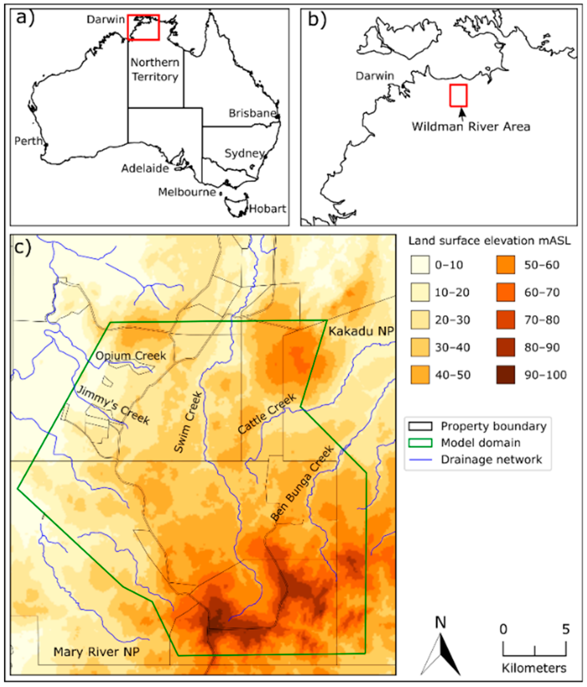
By applying the $\tau$ parameter to capture conceptual uncertainty as described in Section 2.1, the water balance can then be expanded to:

$$\delta =\pm c_1\pm c_2\dots \pm c_{N_C}\pm {\tau }_1{u}_1\pm {\mathsf{\tau }}_2{u}_2\dots \pm {\tau }_{N_U}{u}_{N_U}$$

(7)

where each $u$ represents a conceptually uncertain subcomponent which is associated with a $\tau$ value, and $N_U$ is the number of conceptually uncertain components.

The uncertain components can be organized in a matrix $U$ (Figure 1a) where the number of rows equals the number of uncertain components, $N_U$, while the certain components are organized in the matrix C, where the number of rows equals the number of certain components, $N_C$:

$$U=\left[\begin{array}{cccc}{u}_{1,1}& u_{1,2}& \cdots & u_{1,N_R}\\ u_{2,1}& u_{2,2}& \cdots & u_{2,N_R}\\ ⋮& ⋮& \ddots & ⋮\\ u_{N_U,1}& u_{N_U,1}& \dots & u_{N_U,N_R}\end{array}\right], C=\left[\begin{array}{cccc}{c}_{1,1}& c_{1,2}& \cdots & c_{1,N_R}\\ c_{2,1}& c_{2,2}& \cdots & c_{2,N_R}\\ ⋮& ⋮& \ddots & ⋮\\ c_{N_C,1}& c_{N_C,1}& \dots & c_{N_C,N_R}\end{array}\right]$$

(8)

In both matrices each column represents an individual parameter realization, where $N_R$ is the number of parameter realizations. In each realization the value of the subcomponent will be different, illustrated by the different sizes of the circles in Figure 1a. The magnitude of the subcomponents is modelled stochastically by drawing the value from a predefined prior distribution.

By computing the dot product of T and C and adding $U$, all models can be simulated at the same time for all parameter vectors. This will yield a matrix Δ in which each row presents realizations within each individual conceptual model, $k_j$ with $j\in \left\{1,\dots ,m\right\}$ and each column represents an individual realization based on different parameter vectors ${\theta }_i$ with $i\in \left\{1,\dots ,N_R\right\}$ (Figure 1a):

$$\Delta =T·C+U=\begin{array}{c}\left[\begin{array}{cccc}{\delta }_{1,1}& {\delta }_{1,2}& \cdots & {\delta }_{1,N_R}\\ {\delta }_{2,1}& {\delta }_{2,2}& \cdots & {\delta }_{2,N_R}\\ ⋮& ⋮& \ddots & ⋮\\ {\delta }_{p,1}& {\delta }_{p,2}& \dots & {\delta }_{p,N_R}\end{array}\right]\begin{array}{c}{k}_1\\ k_2\\ ⋮\\ k_p\end{array}\\ \begin{array}{ccccc}{\theta }_{p,1}& {\theta }_{p,2}& \dots & {\theta }_{p,N_R}& \end{array}\end{array}$$

(9)

In Figure 1a, a zero in the T matrix will exclude the subcomponent in matrix Δ while a 1 will include the subcomponent illustrated by the presence and absence of the coloured circles in matrix Δ. This setup of the water balance problem takes advantage of parallelization and vectorization, enabling millions of random realizations to be realized per second. The metropolis sampling algorithm described in Section 2.1 can be defined on top of the already generated realizations by sequentially stepping through the columns of the matrix (Figure 1b). The proposed model $k^{\prime }$ is randomly chosen with weights according to the likelihoods of the different models based on the same parameter vector.

Likelihoods ($p\left(Y|k,{\theta }_k\right)$) can be computed based on the error of the water balance in matrix Δ. The water balance error $\delta$ is scaled to the magnitude of the input to the water balance ($Q_{\mathrm{Input}}$) to get a relative error. By using the relative error, a larger error is accepted for water balances with large water balance components, and a smaller error for water balances with small water balance components. All priors will be constrained by data, so that all samples of the magnitude of the water balance components are considered plausible.

The relative error term is assumed to be normally distributed with a mean of 0 and a standard deviation $\sigma$:

$$p\left(Y|k,{\theta }_k\right)=\frac{1}{\sqrt{2\pi {\sigma }^2}}\exp \frac{{\left(\frac{\delta }{Q_{Input}}-0\right)}^2}{2{\sigma }^2}$$

(10)

The observation error is here assumed to be captured by the parameters set of the prior probabilities of parameter values and $\sigma$ is therefore only related to the remaining conceptual error in the model representing the unknown unknown conceptual components. The standard deviation of the water balance error directly controls the acceptance rate of the water balance realizations; as $\sigma$ increases, more realizations will be accepted. It should be stated that as for all error formulas, errors of an opposite sign will cancel out, reducing the overall error, and a conceptual model with many unknown unknowns might therefore perform well in this framework.

As the magnitude and number of unknown unknowns in the model is unknown, there is no way of determining the value of $\sigma$. The robustness of model ranking as defined by [48], was evaluated in a sensitivity analysis by varying the standard deviation of the relative error of the water balance between 0% and 10%. To avoid making wrong model selection decisions based on the results, we selected a standard deviation of the model error that is least decisive. That is, the difference between the probability of the null and the alternative hypotheses are closest to each other. The least decisive value is the most conservative choice when the model objective is to differentiate between models. From the sensitivity analysis we determined that the most conservative value is $\sigma$ = 2.5%.

3. Case Study

The Wildman River area (Northern Territory, Australia) was chosen as the case study area (Figure 2). The area covers about 400 km² in the northern part of the Northern Territory, next to the Kakadu National Park, between latitudes 12.77° S and 12.47° S and between longitudes 131.7° E and 131.93° E.

The topography in the catchment is relatively flat, and ranges from 100 m above sea level (ASL) in the south to 20 m ASL in the north (Figure 2). Most of the land use is limited to cattle grazing and conservation. Mary River National Park lies south-west of the area and Kakadu National Park to the east. The area has a tropical climate with about 98% of annual precipitation (1450 mm) occurring in the wet season, December to April [49].

The basement geology in the region mainly consists of three units of the Mount Partridge Group which is a part of the Pine Creek Orogen: the Wildman Siltstone, the Koolpinyah Dolostone and the Mundogie Sandstone. The basement is tight to isoclinally folded with a strike of between 180 and 200 degrees. Unconsolidated sediments deposited in the Money Shoal Basin are unconformably overlaying the basement. These sediments are flat laying but repeated incision and infill through the Cenozoic is thought to have created two southwest–northeast oriented palaeovalleys [50], referred to as Mesozoic–Cenozoic (Mz/Cz) sediments, as ambiguity surrounds their age.

The main aquifers consist of a semi-confined Mz/Cz sand aquifer and a confined dolostone aquifer that are assumed to be connected, supported by similarity in hydrogeochemistry [50]. Very limited topographical and piezometric data in the area suggest that the main flow direction is vertical with a very slow horizontal component.

Two major investigations were carried out in the area by the Northern Territory Department of Environment and Natural Resources in relation to a water resource assessment for the area [50] and CSIRO as part of the Northern Australia Water Resources Assessment [49,51]. Tickell and Zaar provided a first-order assessment of the regional-scale groundwater balance [50], while Turnadge et al. provided a refinement of water balance components and a conceptual model [49].

In Section 3.1, we will present the components that constitute the groundwater balance of the Wildman River area. The different components will be computed based on parameter values described in Section 3.2 and on the alternative conceptual models described in Section 3.3. The parameter values and conceptualizations used here are based on the abovementioned investigations.

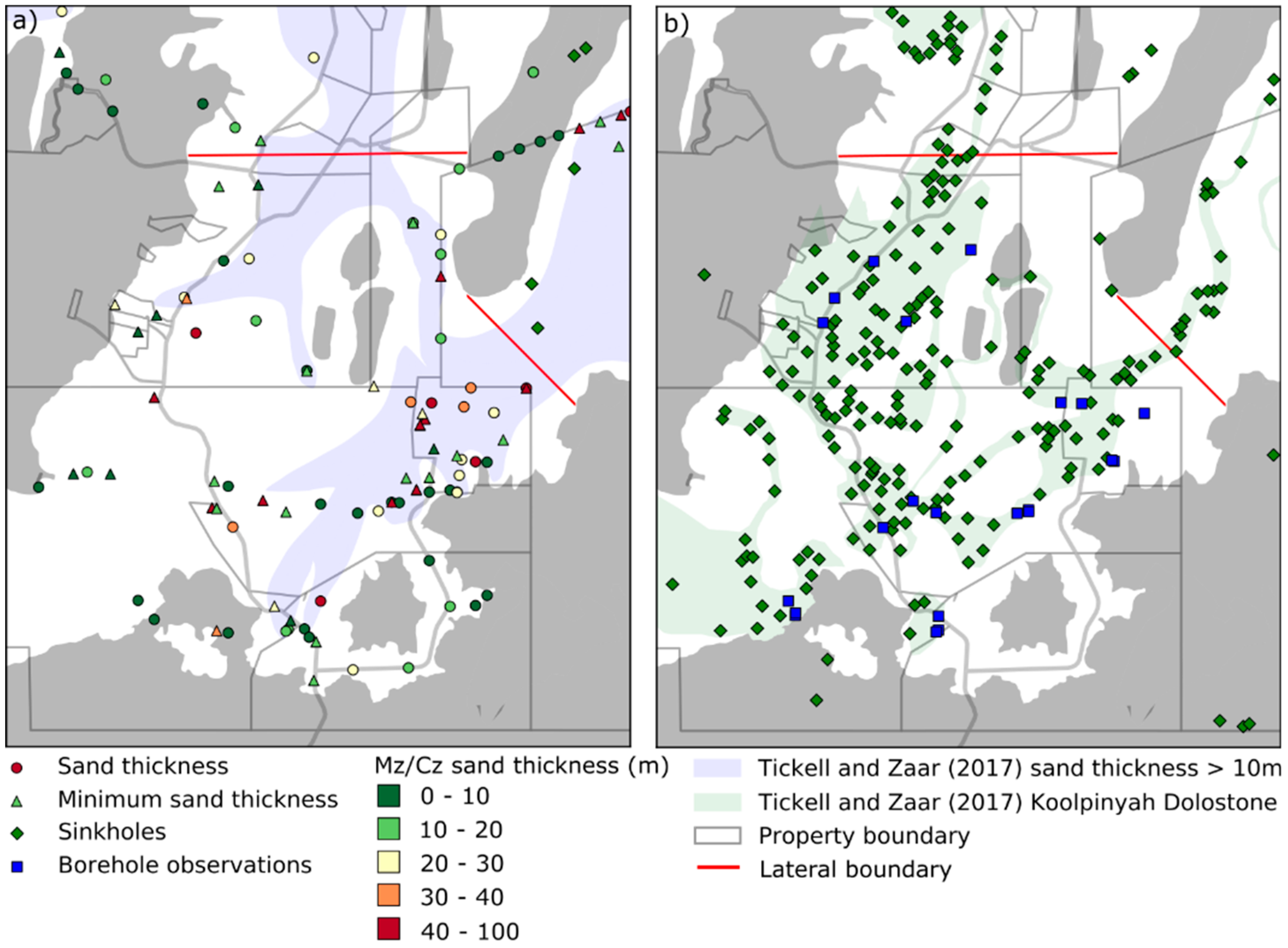
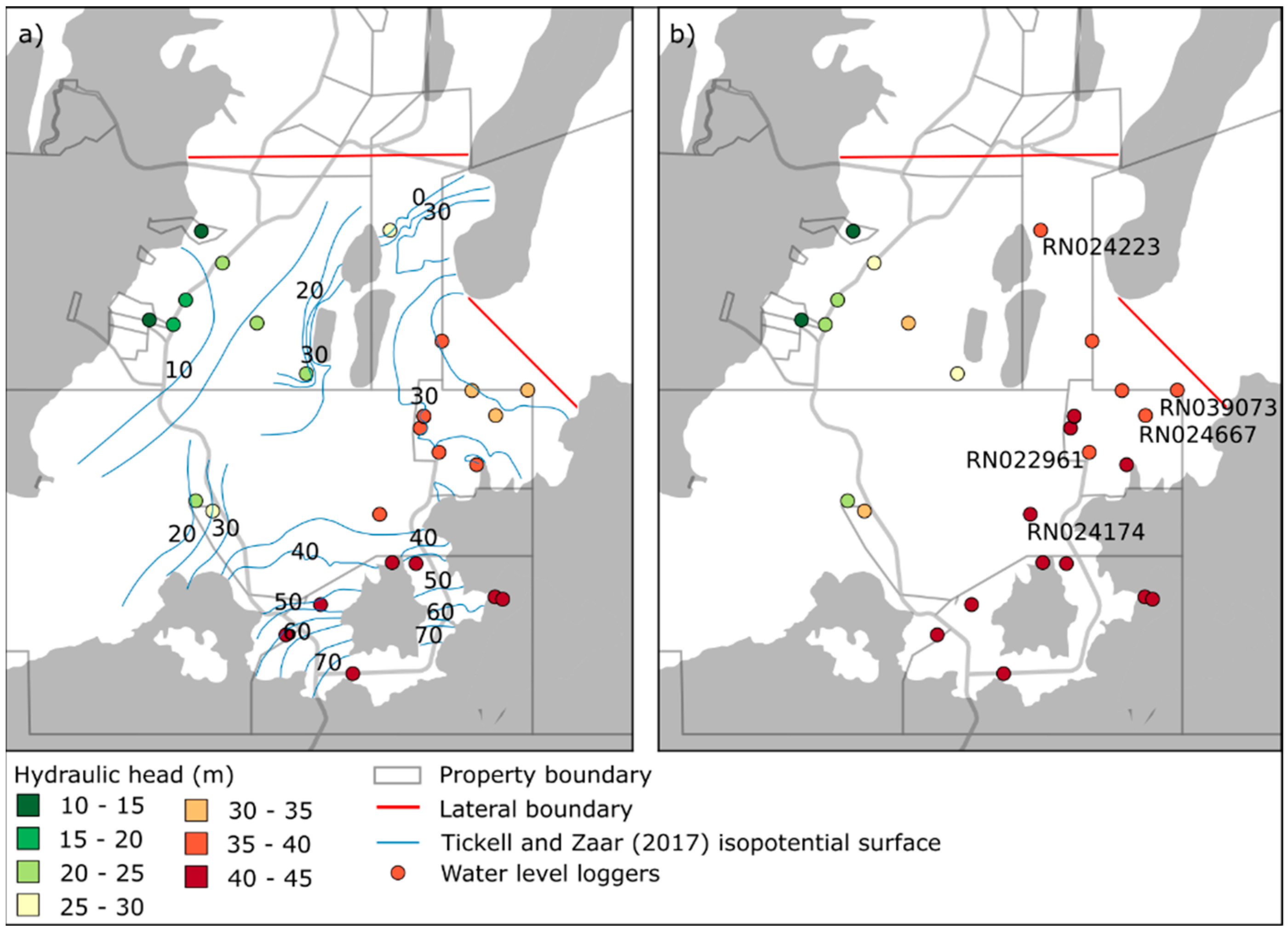
3.1. Water Balance Components

The simplified groundwater balance of the Wildman River area is written as:

$$0=Q_R-Q_L-Q_B+\Delta S+\delta$$

(11)

where $Q_R$ is the net recharge to the water table from rainfall accounting for the losses due to plant transpiration and/or direct soil evaporation [52]. Net recharge is calculated based on a recharge area ($A_R$) and a recharge rate ($R_R$):

$$Q_R=A_R·R_R$$

(12)

$Q_L$ is the lateral groundwater outflow from the aquifers to adjacent areas. The lateral outflow for the Wildman River area is calculated through cross-sections based on Darcy’s law. Darcy’s law depends on the transmissivity of the aquifer ($T_l$), the width of the aquifer ($W_l$) and the hydraulic gradient perpendicular to the cross-section ($\Delta h_l$):

$$Q_L=T_l·W_l·\Delta h_l$$

(13)

The lateral discharge consists of up to four subcomponents: lateral discharge across a northern boundary and a north-eastern model domain boundary, through the Mz/Cz sand aquifer and finally through the Koolpinyah Dolostone aquifer (Figure 3). The remaining boundaries in the model domain in the south and northwest arebounded by impermeable (an order of magnitude less transmissive) bedrock.

$Q_b$ is the baseflow from the aquifer to streams and lagoons. In every time step ($t$), total streamflow ($y_t$) consists of overland flow that reaches the stream quickly, hence named quick flow ($f_t$), and baseflow ($Q_B$) that originates from groundwater discharge. The fraction of the streamflow that makes up the baseflow component is described by the baseflow index $(\beta$) [53]:

$$Q_{B,\mathrm{streams}}=y_t-f_t=\beta ·y_t$$

(14)

The baseflow to streams consist of up to five subcomponents: Jimmy’s Creek, Opium Creek, Swim Creek, Cattle Creek and Ben Bunga Creek (Figure 3). The groundwater discharge to lagoons can be calculated based on seepage rate ($R_L$) and lagoon area ($A_L$):

$$Q_{B,\mathrm{lagoons}}=A_L·R_L$$

(15)

The same seepage rate is assumed for all lagoons in the area.

The final water balance component relates to groundwater storage, $\Delta S$. Based on the observations, the groundwater level returns to a similar level after each year [49] and the annual storage is assumed to be around 0 m³.

For the Wildman River area, transient data for each of the water balance components is scarce, therefore a steady-state water balance is considered. However, the Wildman River area is quite dynamic as the aquifers are filled up in the wet season by the high rainfall events and starts emptying again in the dry season when only very limited rainfall occurs. Given the large difference between the wet and dry season, we will set up a steady-state water balance for both the end of the dry season (1 December) and the end of the wet season (1 April). The wet season and dry season model will be combined into an annual model, so that:

$$\delta =\left(Q_{R,\mathrm{wet}}+Q_{R,\mathrm{dry}}\right)-\left(Q_{L,\mathrm{wet}}+Q_{L,\mathrm{dry}}\right)-\left(Q_{B,\mathrm{wet}}+Q_{B,\mathrm{dry}}\right)+(\Delta S_{\mathrm{wet}}+\Delta S_{\mathrm{dry}})$$

(16)

3.2. Water Balance Parameters

An overview of the parameter values used in the stochastic water balance model is shown in

Table 2. Parameter values describing the water balance components in the Wildman River area. The parameters are described with a uniform distribution between the minimum and the maximum value in the dry and wet season. Parameters that describe areas, width and transmissivities are constant over the year, and therefore only described by one set of a minimum and a maximum value. The term sand refers to Mesozoic–Cenozoic (Mz/Cz) sand, while the term Dolostone refer to the Koolpinyah Dolostone.

Component	Parameter	Dry Min	Dry Max	Wet Min	Wet Max	Unit
Net Recharge	Rate	0	0	32	178	mm/year
	Area	350	400	350	400	km2
Lateral discharge	Transmissivity Dolostone	109	2630	109	2630	m2/day
	Transmissivity Sand	163	1920	163	1920	m2/day
	Gradient North	0.0003	0.0009	0.0004	0.0012	-
	Gradient Northeast	0.0002	0.002	0.0004	0.004	-
	Width Dolostone North	3000	10,000	3000	10,000	m
	Width Dolostone Northeast	1000	7000	1000	7000	m
	Width Sand North	1000	13,000	1000	13,000	m
	Width Sand Northeast	1000	7000	1000	7000	m
Lagoons	Area	2.9	3.2	2.9	3.2	km2
	Rate	0.5	2	0.5	2	mm/day
Streams/springs	Baseflow Jimmy’s Creek	0.06	0.09	0.2	0.3	m3/day
	Baseflow Opium Creek	0.05	0.07	0.2	0.3	m3/day
	Baseflow Swim Creek	0.03	0.1	0.7	2.1	m3/day
	Discharge Cattle Creek	0.001	0.005	0.005	0.03	m3/day
	Discharge Ben Bunga Creek	0.001	0.005	0.005	0.03	m3/day
	Base Flow Index	0.22	0.81	0.22	0.82	-
Annual storage		0	0	0	0	-

. A discussion of the derivation of the prior parameter distributions is found in Appendix A. Uniform distributions are used for all parameters defined by the minimum and maximum value, so that all parameter values in the ranges are equally likely. All the defined rates are used as spatial averages over the whole area.

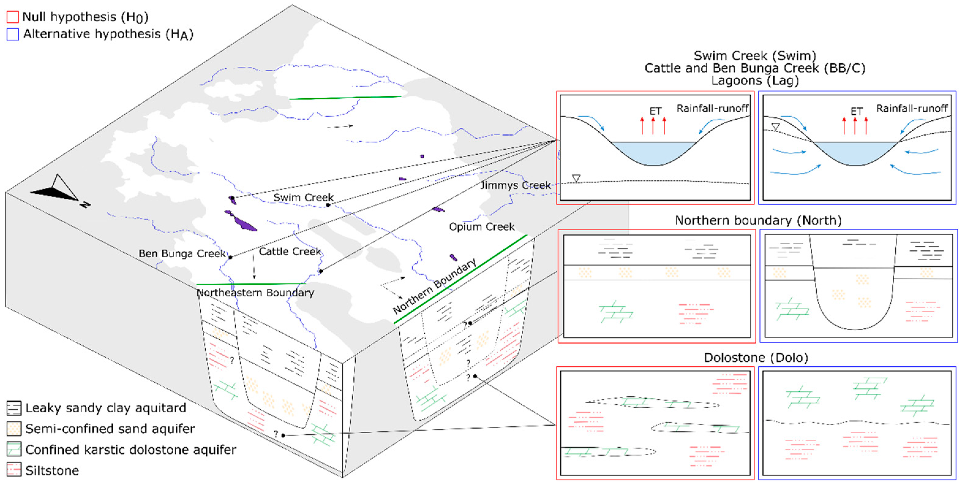
3.3. Alternative Conceptual Models

Even though many investigations [49,50,51] were carried out in the Wildman River area recently, there are still several open conceptual questions. In this paper we focus on the conceptual issues that have a direct influence on the annual water budget of the catchment. In the following discussion, five uncertain water balance components will be identified, and alternative hypotheses will be defined that demonstrate the conceptual issues; in a subsequent step their influence on the water balance will be quantified. The definition of hypotheses will be based on the method specified in Section 2.1. An overview of the conceptual model and conceptual uncertainties in the Wildman River area is shown in Figure 3.

Given the spatially sparse groundwater level observations in the study area, the groundwater flow around the northern boundary of the system can be interpreted in different ways. In one instance [50], groundwater was considered to flow north across the boundary along a northern palaeovalley (i.e., out of the domain) contributing to lateral discharge in the water balance. However, observations may also indicate a northeastward groundwater flow, in which case groundwater will flow along the northern boundary rather than across, resulting in limited lateral discharge across the boundary. Two alternative hypotheses regarding the northern boundary component of lateral discharge are defined:

• H₀: A northern palaeovalley does not exist and the groundwater flows along (i.e., parallel to) the northern boundary of the system and therefore no lateral discharge into or out of this area occurs.
• H_A: A northern palaeovalley exists and the groundwater flows across the northern boundary and therefore contributes to the total lateral discharge out of the model domain.

Based on borehole observations and the location of what is inferred to be sinkholes developed above the Dolostone, Tickell and Zaar interpreted the extent of the Koolpinyah Dolostone as a relatively continuous aquifer [50]. However, the fact that the basement geology including the Koolpinyah Dolostone is folded tightly indicates the plausibility that the Dolostone aquifer consist of more or less structurally isolated aquifers. In this case only the Mz/Cz sand aquifer would contribute to lateral discharge while the Dolostone aquifer would not. This leads to the following hypotheses regarding the Dolostone component of lateral discharge:

• H₀: The Koolpinyah Dolostone is a compartmentalized aquifer and therefore its contribution to lateral discharge is unimportant.
• H_A: The Koolpinyah Dolostone is a continuous aquifer and contributes significantly to lateral discharge.

Ben Bunga and Cattle Creek are ephemeral streams that drain northeastward towards Kakadu National Park. They cease to flow in the early dry season but maintain several isolated permanent pools that are hypothesized to receive groundwater flow through diffuse streambed discharge [50]. However, their ephemeral nature makes this a questionable assumption. It is considered very unlikely that only one of these creeks would receive groundwater and the other not; therefore, the hypotheses for both creeks are combined into a single one:

• H₀: Ben Bunga and Cattle Creek are a rainfall-runoff feature, disconnected from the groundwater system.
• H_A: The streamflow in Ben Bunga and Cattle Creek originates from both groundwater discharge and rainfall-runoff.

Swim Creek is an ephemeral stream that drains the central region of the Wildman River area and flows northward. It ceased to flow at the end of the dry season in 15 out of 29 years of the recorded stream flow. The baseflow index was previously estimated to be around 50% [50]. A different conclusion was obtained by comparing the streamflow record from Swim Creek to that from Opium Creek [49]: streamflow for the former is generally an order of magnitude larger than that for the latter. This was attributed to the much larger surface water catchment of Swim Creek, which led to the assumption that Swim Creek is primarily fed by rainfall-runoff. The hypotheses regarding Swim Creek are defined as follows:

• H₀: Swim Creek is a rainfall-runoff feature, disconnected from the groundwater system.
• H_A: Streamflow in Swim Creek originated from groundwater as well as rainfall-runoff.

A large number of shallow depressions exist in the Wildman River area that are interpreted to be sinkholes formed on top of the Koolpinyah Dolostone [50]. Some of these shallow depressions serve as permanent water features, referred to as lagoons, which led Turnadge et al. to hypothesize that they are groundwater discharge features [49]. However, using a mass balance approach, groundwater discharge to the lagoon was found to only occur during wetter than average climate conditions [50]. Until date, only the largest of the Twin Sisters Lagoons has been subject to investigations, involving the comparison of lake stage recession to evaporation rate [54]. Based on one year of observations, it was estimated that the lagoon was a flow-through feature. In yet another study, analysis of the noble gas tracer Rn-222 in surface water samples collected from the lagoon, also did not yield conclusive results in regards to whether or not groundwater inflow occurs [49]. These ambiguous findings around potential groundwater contribution to the Twin Sisters Lagoon makes this an important conceptual uncertainty. The other permanent lagoons in the area (Number One Billabong, Lake Lucy and Mistake Billabong) are assumed to behave in the same way as the Twin Sisters Lagoons. The hypotheses regarding permanent lagoons are defined as follows:

• H₀: The permanent lagoons are rainfall-runoff features, disconnected from the groundwater system.
• H_A: The permanent lagoons are, at least in part, groundwater discharge features.

In the above discussion, a total of five uncertain water balance components were identified, while two alternative models were defined for each uncertain component. Using the factorial design approach described in Section 2.1 thus gives 2⁵ or 32 individual models that will be quantitatively evaluated.

We assign a uniform prior probability to the 32 alternative combinations (i.e., all models are considered equally likely). By using uniform priors, we expect that the evaluation of internal model consistency expressed as the likelihood function (Section 2.4) dominates the resulting posterior distribution. Alternatively, the prior could have been based on an expert elicitation process, as in (e.g., [55,56]), to be able to further differentiate between the models. However, the scope of the paper is to evaluate whether there is enough information in the water balance to offer insight into the conceptualizations. Expert elicitation of the prior probabilities is therefore beyond the scope of this paper.

4. Results

In this section, we apply the Bayesian hypothesis testing framework to the stochastic water balance in the case study. On a 2.4 GHz computer with 8 GB RAM every 10,000 realisations take ~1 s with an acceptance rate of the water balance realizations of ~27%. A graphical description of the setup of the model is seen in Figure 1. The illustration shows that the forward model (i.e., the groundwater balance problem), is linear and additive, and the setup allows for vectorization and parallelization, which allows for evaluation of a large set of model versions. All implementations, calculations and sampling is performed in the Python 3.6 computing environment with the software stack of NumPy [57] while the figures are prepared with Matplotlib [58]. The script is available as supplementary material.

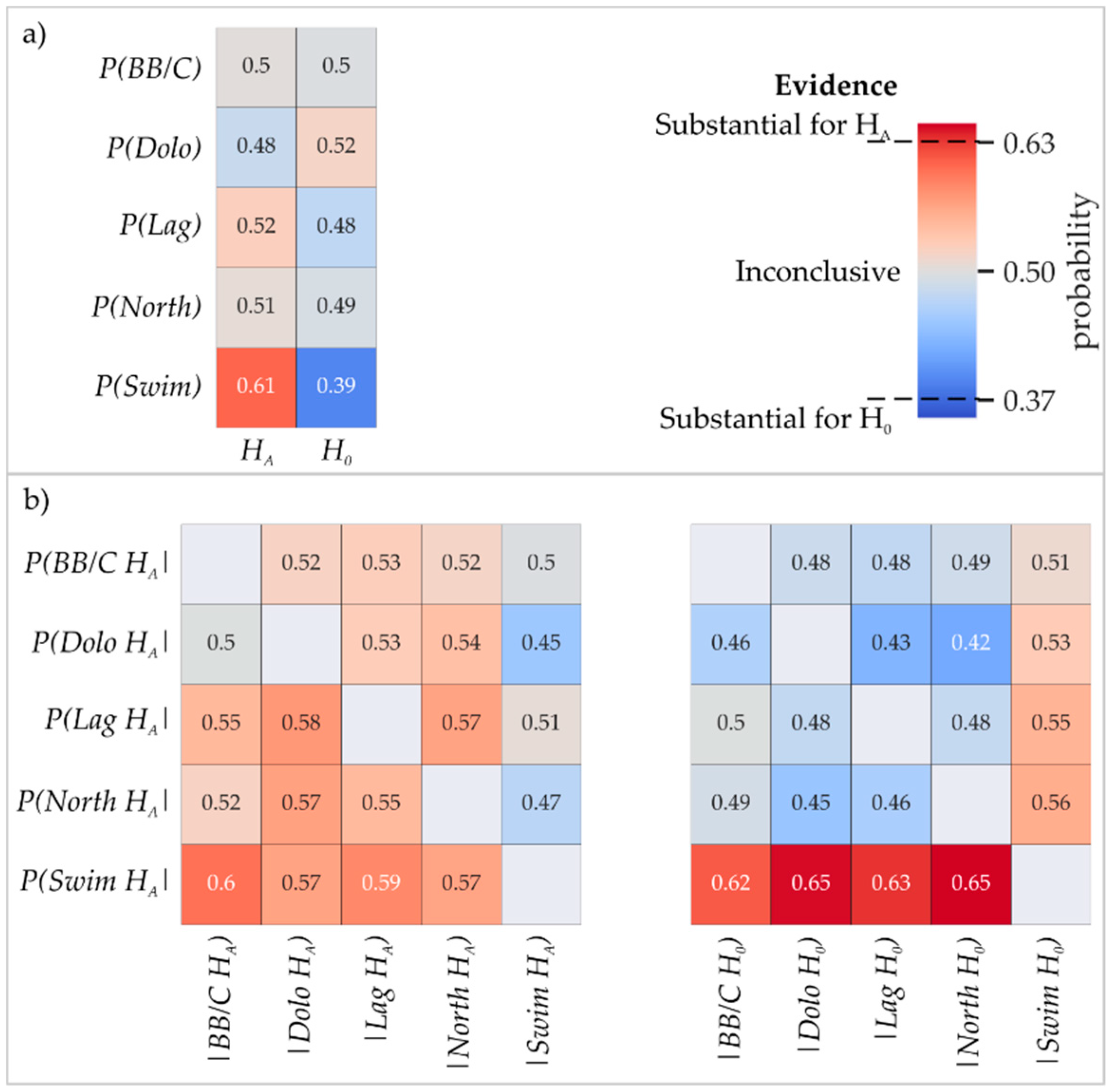
4.1. Posterior Probabilities of Hypotheses based on Assumed Error

The simple and conditional probabilities for the alternative hypotheses (H_A) are shown in Figure 4. The simple probability shown in Figure 4a is the marginal probability of a subset of 16 out of 32 different models (H₀ vs. H_A). The conditional probability shown in Figure 4b is the marginal probability of a subset of 8 out of 32 different models that meets the conditions described in the parentheses. The corresponding probabilities for the null hypotheses (H₀) (only shown for Figure 4a) can be obtained as 1 subtracted by the probabilities for an alternative hypothesis. By applying Bayesian hypothesis testing, we have implicitly assumed that a quasi-true model can be identified from the alternative model ensemble [17]. Given more data, the probabilities for H_A or H₀ would therefore further approach either 1 or 0.

The simple probabilities (Figure 4a) show that a clear preference for the alternative hypothesis is supported only for the conceptually uncertain Swim Creek with a value of 39% and 61% for the null and alternative hypotheses, respectively. The support can, however, still only be described as “Inconclusive” (Section 2.3), based on a Bayes factor of less than 3 (63.5%, Table 1). For the rest of the conceptual uncertain components, the change between the prior probability of 0.5 and the posterior probability is even smaller. This indicates that the information content in the closure of the water balance is too small to sufficiently differentiate between models in order for valid model rejection to occur. A balanced water budget can result from sufficiently accounting for all water balance components, but can also arrive from globally balanced errors [26]. The results therefore suggest that without other constraints, all suggested conceptual models are valid because they are either true or can sufficiently balance errors in the conceptualization globally. A possible strategy to increase model discrimination is to further constrain parameter priors by collection of more data [40]. With further constraints on the parameter priors (i.e., reduction of parameter ranges in Table 2), the ability of the different models to balance errors globally reduces as the magnitude of the water balance components will vary less. Another strategy to increase the ability to differentiate between models is to apply informed priors, but as already stated in Section 3.3, this is beyond the scope of this paper.

The conditional probabilities (P(X|Y)) (Figure 4b) describe the probability of a hypothesis X given the assumption that another hypothesis Y is true. It thereby offers a preview of how the probabilities would change for hypothesis X if we found hypothesis Y to be true (e.g., by collecting additional data).

Provided the alternative hypothesis of any uncertain component, but Swim Creek, the conditional probabilities are higher in case an alternative hypothesis (P(X H_A|Y H_A)) rather than a null-hypothesis (P(X H_A|Y H₀)) is used as the other given event (i.e., other uncertain component). This indicates a general preference for applying more components to balance the water budget. That is, if none of the additional uncertain discharge components (alternative hypotheses) are applied, there is a surplus in the water balance. However, when the Swim Creek model component is involved, a trade-off with the remaining alternative hypotheses can be observed. This is especially true for the conditional probability of the alternative hypothesis for Swim Creek given the Dolostone (P(Swim H_A|Dolo H₀)) and the northern boundary (P(Swim H_A|North H₀)) hypotheses, where the support becomes “substantial” (both 0.65), when the null-hypotheses are applied. This indicates that the input to the water balance is not large enough to account for both the alternative hypotheses for Swim Creek and the Dolostone or Northern boundary, that all include extra discharge terms. In conclusion, the largest change in conditional probability can be observed for when Swim Creek is involved, and future field work should therefore aim at resolving this conceptual uncertainty first.

4.2. Model Predictions

The prior and posterior predictions for recharge, lateral discharge and baseflow as obtained from the stochastic water balance calculations are shown in the top row of Figure 5. The obtained predictions represent a multi-model probability density function that takes account of all the conceptual models that seem plausible under the current state of knowledge as well as the parameter uncertainty. These results are compared with the deterministic estimates for the different water balance components in [50], which provided two independent water balance estimates, shown as vertical lines in Figure 5.

Compared to the deterministic solutions from [50], the posterior probability has not changed significantly. However, in our stochastic predictions both parameter and conceptual uncertainty are accounted for. We therefore have a water balance of which the confidence limits are quantified.

The prior probability for baseflow is highly bimodal, caused by the trans-dimensional sampling between models that include extra baseflow components (alternative hypotheses for Ben Bunga and Cattle Creek, Lagoons and Swim Creek) and the models that exclude the extra baseflow component (corresponding null hypotheses). The prior probability for recharge and lateral discharge is however unimodal, suggesting that the conceptual uncertainty is of less importance than the parameter probability.

The posterior probability for recharge and baseflow is multimodal (Figure 5, top row). While the prior probability for the baseflow is already multimodal, the prior for recharge is not and the shape of the posterior is therefore caused by the conditioning to the closure of the water balance. Overall the range of the posterior of the recharge is shown to be reduced to a maximum of 60 GL/year, whereas the maximum for the prior distribution is 70 GL/year. However, the posterior probability of the lateral discharge and baseflow has not changed significantly, indicating low information in data (the balancing of the water budget), because a trade-off exists between the output components. Both lateral discharge and baseflow are loss terms in the water balance that will respond in a similar way when poorly defined parameter distributions are used, as is the case here.

The impact of different hypotheses on the simulated recharge, lateral discharge and baseflow is shown in Figure 5; each row represents posterior probability subdivided into the models that includes the null and the alternative hypotheses (16 models each) for one of the five uncertain components, as referenced in the row header. The within model variance is represented by either the red or blue probability distribution depending on the chosen model, while the between-model variance is represented by the difference between the red and the blue probability distribution.

In three out of five cases, we can observe an increase in the amount of recharge that can be supported in the model when an alternative hypothesis (blue) is applied, as all alternative hypotheses add an extra discharge component to the water balance. In only two cases recharge does not increase: for the conceptual uncertainty regarding Ben Bunga and Cattle Creek (row BB/C) and the Lagoons (row Lag). While these components directly impact the baseflow prediction, they are shown to have very little impact on recharge and lateral discharge. The conceptual uncertainty regarding the Dolostone (row Dolo) and the northern lateral boundary (row North), both directly impacting the lateral discharge prediction, is however shown to have a more pronounced indirect impact on recharge (i.e., the probability distribution shifts to higher values by about 10 GL/year). The largest impact on the overall predictions is, however, caused by the conceptual uncertainty regarding Swim Creek (row Swim). The trans-dimensional sampling between including and excluding the discharge component from Swim Creek hypothesis directly impacts baseflow, which becomes bimodal, and thereby indirectly affects the prediction of recharge which also becomes bimodal.

Again, it is shown that the reduction of uncertainty would be greatest if we were able to resolve the Swim Creek conceptual uncertainty (e.g., by additional field work). The additional field work could target Swim Creek directly, but it could also aim at reducing the aleatory uncertainty of the net recharge component. Figure 5 shows that if the net recharge to the area is more than 40 GL/year the alternative hypothesis for Swim Creek is true. However, if the net recharge to the area is less than 20 GL/year, the null hypothesis for Swim Creek would be true.

5. Discussion

The results presented in Section 4 are consistent with what is presented in other groundwater modelling studies (e.g., [11,12,15,59,60,61]), in that we have obtained posterior model probabilities and a probability distribution of predictions including both parameter and conceptual uncertainty. However, the methods with which these model results have been obtained, differ. The advantages and disadvantages of our approach compared to the abovementioned studies are discussed in the following.

We applied a factorial design approach, where all possible combinations of hypotheses are tested, which enables the attribution of differences in model performance, directly to specific conceptually uncertain components. The factorial design approach is capable of isolating the causes affecting the model predictions. However, as every new conceptually uncertain component doubles the number of possible models (assuming two hypotheses are defined for each uncertain component), the problem can quickly become time consuming. This practical barrier is referred to as the fallacy of factorial design in [62].

To avoid making the problem numerically intractable, we have applied a very simple additive and linear model setup (rather than a 3D numerical groundwater flow or transport model), which enables us to run millions of models in a matter of seconds. The studies we compare our results to run between 4000 and 300,000 realizations. By being able to run more realizations, we ensure a more stable result and that there is no practical limitation to how many different conceptual models can be evaluated. The simplicity of the model setup allows us to gain insight, without undue amount of time, which can be brought forward into subsequent more complex modelling.

The disadvantage of our simple approach is that the data the models are tested against is limited. In the applied setup the only data used to evaluate the models against, is the assumption that the water budget is balanced. All other data in the case study were used to set up the priors for the parameters describing the water balance. In contrast, the abovementioned studies included testing data such as hydraulic head, contaminant concentrations and pumping tests. The limited available evaluation data in the suggested approach means that we will not be able to discriminate between models to the same extent as the abovementioned studies. To improve the discriminatory power of this modelling approach more data should be reserved for model evaluation.

The model cannot underpin environmental management but is an initial screening tool built to allow the modeler to gain insight into the system functioning, identify important sources of uncertainty and prioritize research efforts. In a stepwise approach to groundwater modelling (discussed in Section 1), the suggested approach would constitute one of the initial steps after the hydrogeological characterization before moving towards testing a more complex mathematical model. This model testing step would then inform the succeeding steps ensuring a transparent workflow.

6. Conclusions

We presented an approach to model-based Bayesian hypothesis testing in a simple additive groundwater balance model, which involves optimization of a model in function of both parameter values and a conceptual model. The proposed systematic conceptual model development method allows for directly attributing the differences in performance of alternative models to individual uncertain components in the conceptual model.

The method was demonstrated on a water balance model for the Wildman River area. Five conceptually uncertain components resulted in 32 individual conceptual models and millions of realizations with all conceptualizations being conditioned to the closure of the water balance. The following can be concluded from the case study:

• More confidence was gained in the water balance compared to the deterministic solution. Probabilistic distribution of predictions take account of all the conceptual models that seem plausible under the current state of knowledge as well as the parameter uncertainty.
• The understanding of the system functioning has increased. None of the conceptual models can be ruled out, but we have a better idea of how important they are to the water balance predictions and how they impact parameter ranges.
• The fieldwork going forward can now be prioritized in terms of the impact the different components have shown on the water balance predictions.

Testing alternative conceptual models is recognized to increase transparency, help prioritize research effort and help uncover potential conceptual surprises. The overall conclusion of this study is that testing alternative conceptual models does not have to be a time-consuming task but can be done in relatively simple models (e.g., as here, in a water balance model).

References

1. Gupta, H.V.; Clark, M.P.; Vrugt, J.A.; Abramowitz, G.; Ye, M. Towards a comprehensive assessment of model structural adequacy. Water Resour. Res. 2012, 48, 1–16. [Google Scholar] [CrossRef]
2. Enemark, T.; Peeters, L.J.M.; Mallants, D.; Batelaan, O. Hydrogeological conceptual model building and testing: A review. J. Hydrol. 2019, 569, 310–329. [Google Scholar] [CrossRef]
3. Bredehoeft, J.D. The conceptualization model problem-surprise. Hydrogeol. J. 2005, 13, 37–46. [Google Scholar] [CrossRef]
4. Beven, K.J. On hypothesis testing in hydrology: Why falsification of models is still a really good idea. WIREs Water 2018, 3, e1278. [Google Scholar] [CrossRef]
5. Nearing, G.S.; Gupta, H.V. Ensembles vs. information theory: Supporting science under uncertainty. Front. Earth Sci. 2018, 12, 653–660. [Google Scholar] [CrossRef]
6. Oreskes, N.; Shrader-frechette, K.; Belitz, K. Verification. Validation and Confirmation of Numerical Models in the Earth Sciences. Science 1994, 263, 641–646. [Google Scholar] [CrossRef] [PubMed]
7. Caers, J. Bayesianism in Geoscience. In Handbook of Mathematical Geosciences; Sagar, B.S.D., Cheng, Q., Agterberg, F., Eds.; Springer: Stanford, CA, USA, 2018; pp. 527–566. [Google Scholar]
8. Guillaume, J.H.A.; Hunt, R.J.; Comunian, A.; Blakers, R.S.; Fu, B. Methods for Exploring Uncertainty in Groundwater Management Predictions. In Integrated Groundwater Management; Jakeman, A.J., Barreteau, O., Hunt, R.J., Rinaudo, J., Ross, A., Eds.; Springer: Berlin, Germany, 2016; pp. 602–614. [Google Scholar]
9. Kass, R.E.; Raftery, A.E. Bayes Factors. J. Am. Stat. Assoc. 1995, 90, 773–795. [Google Scholar] [CrossRef]
10. Jeffreys, H. Theory of Probability, 3rd ed.; Oxford University Press: Oxford, UK, 1939. [Google Scholar]
11. Rojas, R.M.; Kahunde, S.; Peeters, L.; Batelaan, O.; Feyen, L.; Dassargues, A. Application of a multimodel approach to account for conceptual model and scenario uncertainties in groundwater modelling. J. Hydrol. 2010, 394, 416–435. [Google Scholar] [CrossRef] [Green Version]
12. Rojas, R.M.; Batelaan, O.; Feyen, L.; Dassargues, A. Assessment of conceptual model uncertainty for the regional aquifer Pampa del Tamarugal–North Chile. Hydrol. Earth Syst. Sci. Discuss. 2010, 6, 5881–5935. [Google Scholar] [CrossRef]
13. Hermans, T.; Nguyen, F.; Caers, J. Uncertainty in training image-based inversion of hydraulic head data constrained to ERT data: Workflow and case study. Water Resour. Res. 2015, 51, 5332–5352. [Google Scholar] [CrossRef]
14. Brunetti, C.; Linde, N.; Vrugt, J.A. Bayesian model selection in hydrogeophysics: Application to conceptual subsurface models of the South Oyster Bacterial Transport. Adv. Water Resour. 2017, 102, 127–141. [Google Scholar] [CrossRef]
15. Troldborg, M.; Nowak, W.; Tuxen, N.; Bjerg, P.L.; Helmig, R.; Binning, P.J. Uncertainty evaluation of mass discharge estimates from a contaminated site using a fully Bayesian framework. Water Resour. Res. 2010, 46, 1–19. [Google Scholar] [CrossRef]
16. Thomsen, N.I.; Binning, P.J.; Mcknight, U.S.; Tuxen, N.; Bjerg, P.L.; Troldborg, M. A Bayesian belief network approach for assessing uncertainty in conceptual site models at contaminated sites. J. Contam. Hydrol. 2016, 188, 12–28. [Google Scholar] [CrossRef] [PubMed] [Green Version]
17. Höge, M.; Guthke, A.; Nowak, W. The hydrologist’s guide to Bayesian model selection, averaging and combination. J. Hydrol. 2019, 572, 96–107. [Google Scholar] [CrossRef]
18. Remson, I.; Gorelick, S.M.; Fliegner, J.F. Computer Models in Ground-Water Exploration. Ground Water 1980, 18, 447–451. [Google Scholar] [CrossRef]
19. Dausman, A.M.; Doherty, J.; Langevin, C.D.; Dixon, J. Hypothesis testing of buoyant plume migration using a highly parameterized variable-density groundwater model at a site in Florida, USA. Hydrogeol. J. 2010, 18, 147–160. [Google Scholar] [CrossRef]
20. Haitjema, H.M. Introduction. In Analytic Element Modeling of Groundwater Flow; Haitjema, H.M., Ed.; Academic Press: Cambridge, MA, USA, 1995; pp. 1–4. [Google Scholar]
21. Neuman, S.P.; Wierenga, P.J. A Comprehensive Strategy of Hydrogeologic Modeling and Uncertainty Analysis for Nuclear Facilities and Sites (NUREG/CR-6805); U.S. Nuclear Regulatory Commission: Washington, DC, USA, 2003; p. 311.
22. Haitjema, H.M. The Role of Hand Calculations in Ground Water Flow Modeling. Groundwater 2006, 44, 786–791. [Google Scholar] [CrossRef]
23. Hunt, R.J.; Zheng, C. The Current State of Modeling. Ground Water 2012, 50, 330–333. [Google Scholar] [CrossRef]
24. Turnadge, C.; Mallants, D.; Peeters, L. Sensitivity and uncertainty analysis of a regional-scale groundwater flow model featuring coal seam gas extraction. CSIRO, Australia. ResearchGate 2018. [Google Scholar] [CrossRef]
25. Refsgaard, J.C.; Christensen, S.; Sonnenborg, T.O.; Seifert, D.; Højberg, A.L.; Troldborg, L. Review of strategies for handling geological uncertainty in groundwater flow and transport modeling. Adv. Water Resour. 2012, 36, 36–50. [Google Scholar] [CrossRef]
26. Dassargues, A. Chapter 2: Hydrologic balance and groundwater. In Hydrogeology: Groundwater Science and Engineering; Dassargues, A., Ed.; CRC Press: Boca Raton, FL, USA, 2018. [Google Scholar]
27. Barnett, B.; Townley, L.R.; Post, V.; Evans, R.E.; Hunt, R.J.; Peeters, L.; Richardson, S.; Werner, A.D.; Knapton, A.; Boronkay, A. Australian Groundwater Modelling Guidelines; National Water Commision: Canberra, Australia, 2012; ISBN 9781921853913. [Google Scholar]
28. Baalousha, H. Stochastic water balance model for rainfall recharge quantification in Ruataniwha Basin, New Zealand. Environ. Geol. 2009, 58, 85–93. [Google Scholar] [CrossRef]
29. Sebok, E.; Refsgaard, J.C.; Warmink, J.J.; Stisen, S.; Jensen, K.H. Using expert elicitation to quantify catchment water balances and their uncertainties. Water Resour. Res. 2016, 52, 5111–5131. [Google Scholar] [CrossRef] [Green Version]
30. Thompson, S.; MacVean, L.; Sivapalan, M. A stochastic water balance framework for lowland watersheds. Water Resour. Res. 2017, 53, 9564–9579. [Google Scholar] [CrossRef]
31. Green, P.J. Trans-dimensional Markov chain Monte Carlo. In Highly Structured Stochastic Systems; Green, P.J., Hjort, N.L., Richardson, S., Eds.; Oxford Statistical Science Series: Oxford, UK, 2003; pp. 179–198. [Google Scholar]
32. Malinverno, A.; Leaney, W. A Monte Carlo method to quantify uncertainty in the inversion of zero-offset vsp data. In Proceedings of the 70th SEG Annual Meeting Expanded Abstracts, Tulsa, Oklahoma, 6–11 August 2000; pp. 2392–2396. [Google Scholar]
33. Jiménez, S.; Mariethoz, G.; Brauchler, R.; Bayer, P. Smart pilot points using reversible-jump Markov-chain Monte Carlo. Water Resour. Res. 2016, 52, 3966–3983. [Google Scholar] [CrossRef] [Green Version]
34. Mondal, A.; Efendiev, Y.; Mallick, B.; Datta-Gupta, A. Bayesian uncertainty quantification for flows in heterogeneous porous media using reversible jump Markov chain Monte Carlo methods. Adv. Water Resour. 2010, 33, 241–256. [Google Scholar] [CrossRef]
35. Somogyvari, M.; Jalali, M.; Parras, S.J.; Bayer, P. Synthetic fracture network characterization with transdimensional inversion. Water Resour. Res. 2017, 53, 5104–5123. [Google Scholar] [CrossRef]
36. Metropolis, N.; Ulam, S. The Monet Carlo Method. J. Am. Stat. Assoc. 1949, 44, 335–341. [Google Scholar] [CrossRef]
37. Hastings, W.K. Monte Carlo Sampling Methods Using Markov Chains and Their Applications. Biometrika 1970, 57, 97–109. [Google Scholar] [CrossRef]
38. Lee, J.; Sung, W.; Choi, J.H. Metamodel for efficient estimation of capacity-fade uncertainty in Li-Ion batteries for electric vehicles. Energies 2015, 8, 5538–5554. [Google Scholar] [CrossRef]
39. Fisher, R.A. The factorial design of experimentation. In The Design of Experiments; Fisher, R.A., Ed.; Oliver and Boyd: London, UK, 1935; pp. 96–113. [Google Scholar]
40. Pham, H.V.; Tsai, F.T.C. Optimal observation network design for conceptual model discrimination and uncertainty reduction. Water Resour. Res. 2016, 52, 1245–1264. [Google Scholar] [CrossRef] [Green Version]
41. Aphale, O.; Tonjes, D.J. Multimodel Validity Assessment of Groundwater Flow Simulation Models Using Area Metric Approach. Groundwater 2017, 55, 219–226. [Google Scholar] [CrossRef] [PubMed]
42. Højberg, A.L.; Refsgaard, J.C. Model uncertainty-parameter uncertainty versus conceptual models. Water Sci. Technol. 2005, 52, 177–186. [Google Scholar] [CrossRef] [PubMed]
43. Seifert, D.; Sonnenborg, T.O.; Refsgaard, J.C.; Højberg, A.L.; Troldborg, L. Assessment of hydrological model predictive ability given multiple conceptual geological models. Water Resour. Res. 2012, 48, 1–16. [Google Scholar] [CrossRef]
44. Ye, M.; Meyer, P.D.; Neuman, S.P. On model selection criteria in multimodel analysis. Water Resour. Res. 2008, 44, 1–12. [Google Scholar] [CrossRef]
45. Tsai, F.T.C.; Elshall, A.S. Hierarchical Bayesian model averaging for hydrostratigraphic modeling: Uncertainty segregation and comparative evaluation. Water Resour. Res. 2013, 49, 5520–5536. [Google Scholar] [CrossRef]
46. Chitsazan, N.; Nadiri, A.A.; Tsai, F.T.C. Prediction and structural uncertainty analyses of artificial neural networks using hierarchical Bayesian model averaging. J. Hydrol. 2015, 528, 52–62. [Google Scholar] [CrossRef] [Green Version]
47. Sambridge, M.; Gallagher, K.; Jackson, A.; Rickwood, P. Trans-dimensional inverse problems, model comparison and the evidence. Geophys. J. Int. 2006, 167, 528–542. [Google Scholar] [CrossRef] [Green Version]
48. Schöniger, A.; Wöhling, T.; Nowak, W. A statistical concept to assess the uncertainty in Bayesian model weights and its impact on model ranking. Water Resour. Res. 2015, 51, 7524–7546. [Google Scholar] [CrossRef] [Green Version]
49. Turnadge, C.; Crosbie, R.S.; Tickell, S.J.; Zaar, U.; Smith, S.D.; Dawes, W.R.; Davies, P.; Harrington, G.A.; Taylor, A.R. Hydrogeological characterisation of the Mary–Wildman rivers area, Northern Territory. In A Technical Report to the Australian Government from the CSIRO Northern Australia Water Resource Assessment, Part of the National Water Infrastructure Development Fund: Water Resource Assessments; CSIRO: Canberra, Australia, 2018; Available online: https://publications.csiro.au/rpr/download?pid=csiro:EP185984&dsid=DS3 (accessed on 16 January 2019).
50. Tickell, S.J.; Zaar, U. Water Resources of the Wildman River Area, Technical Report 8/2017D; Northern Territory Department of Environment and Natural Resources: Palmerston City, Australia, 2017.
51. Turnadge, C.; Taylor, A.R.; Harrington, G.A. Groundwater flow modelling of the Mary–Wildman rivers area, Northern Territory. In A Technical Report to the Australian Government from the CSIRO Northern Australia Water Resource Assessment, Part of the National Water Infrastructure Development Fund: Water Resources Assessments; CSIRO: Canberra, Australia, 2018. [Google Scholar] [CrossRef]
52. Doble, R.C.; Crosbie, R.S. Review: Current and emerging methods for catchment-scale modelling of recharge and evapotranspiration from shallow groundwater. Hydrogeol. J. 2017, 25, 3–23. [Google Scholar] [CrossRef]
53. Eckhardt, K. A comparison of baseflow indices, which were calculated with seven different baseflow separation methods. J. Hydrol. 2008, 352, 168–173. [Google Scholar] [CrossRef]
54. Graham, B. Surface Water Resources in the Northeastern Corner of Wildman River Station (Final Report for Water Resources Division Project Number 2026); Department of Mines and Energy: Darwin, Australia, 1985.
55. Meyer, P.D.; Ye, M.; Rockhold, M.L.; Neuman, S.P.; Cantrell, K.J. Combined Estimation of Hydrogeologic Conceptual Model, Parameter, and Scenario Uncertainty with Application to Uranium Transport at the Hanford Site 300 Area; Pacific Northwest National Lab.: Richland, WA, USA, 2007. [Google Scholar]
56. Ye, M.; Pohlmann, K.F.; Chapman, J.B. Expert elicitation of recharge model probabilities for the Death Valley regional flow system. J. Hydrol. 2008, 354, 102–115. [Google Scholar] [CrossRef]
57. Oliphant, T.E. A Guide to NumPy; CreateSpace Independent Publishing Platform: Scotts Valley, CA, USA, 2006. [Google Scholar]
58. Hunter, J.D. Matplotlib: A 2D Graphics Environment. Comput. Sci. Eng. 2007, 9, 90–95. [Google Scholar] [CrossRef]
59. Rojas, R.M.; Feyen, L.; Dassargues, A. Conceptual model uncertainty in groundwater modeling: Combining generalized likelihood uncertainty estimation and Bayesian model averaging. Water Resour. Res. 2008, 44. [Google Scholar] [CrossRef] [Green Version]
60. Schöniger, A.; Illman, W.A.; Wöhling, T.; Nowak, W. Finding the right balance between groundwater model complexity and experimental effort via Bayesian model selection. J. Hydrol. 2015, 531, 96–110. [Google Scholar] [CrossRef]
61. Zeng, X.; Wang, D.; Wu, J.; Zhu, X.; Wang, L.; Zou, X. Evaluation of a Groundwater Conceptual Model by Using a Multimodel Averaging Method. Hum. Ecol. Risk Assess. Int. J. 2015, 21, 1246–1258. [Google Scholar] [CrossRef]
62. Betini, G.S.; Avgar, T.; Fryxell, J.M. Why are we not evaluating multiple competing hypotheses in ecology and evolution? R. Soc. Open Sci. 2017, 4, 160756. [Google Scholar] [CrossRef] [Green Version]
63. Cook, P.G.; Bohlke, J.-K. Determining Timescales for Groundwater Flow and Solute Transport. In Environmental Tracers in Subsurface Hydrology; Cook, P.G., Herczeg, A.L., Eds.; Springer: Berlin, Germany, 2000; pp. 1–30. ISBN 9781461370574. [Google Scholar]
64. Lyne, V.; Hollick, M. Stochastic Time-Variable Rainfall-Runoff Modeling. In Proceedings of the Institute of Engineers Australia National Conference, Perth, Australia, September 1979; Available online: https://www.researchgate.net/publication/272491803_Stochastic_Time-Variable_Rainfall-Runoff_Modeling (accessed on 23 January 2019).
65. Eckhardt, K. How to construct recursive digital filters for baseflow separation. Hydrol. Process. 2005, 19, 507–515. [Google Scholar] [CrossRef]
Figure 1. (a) Method for calculation of the water balance error, Δ . The colours of the circles represent different system subcomponents, C, while the size of the circles represents the magnitude of the subcomponent in each realization, θ i with i { 1 , , N R } where N R is the number of variable realizations. The combination of τ h with h { 1 , , N U } , where N U is the number of uncertain model components, in the rows of T , constitutes a model, k j with j { 1 , , m } where m = 2 N U . The uncertain model components in U includes N U components, while the certain model components in C includes N C components. (b) Metropolis–Hastings sampling of the water balance realizations. The circles and arrows represent those that are accepted or rejected based on the acceptance criteria, α . The dotted circles and arrows represent proposed moves that were not accepted. Figure 1b modified from [38].
Water 11 01463 g001
Figure 2. The study area is a part of the Wildman River area located between Mary River and Kakadu National Park in Northern Territory, Australia. (a) Australia, (b) North-western part of Northern Territory, (c) Wildman River Area.
Water 11 01463 g002
Figure 3. Conceptually uncertain components in Wildman River area and hypotheses developed to characterize the conceptual uncertainty.
Water 11 01463 g003
Figure 4. Simple (a) and conditional (b) posterior probabilities of hypotheses concerning uncertain water balance components. (b) Should be read: probability of row, given column (e.g., P(Dolo HA|North HA)). In (b) the inverse probability (not shown here) is P(X H0|Y HA) = 1 − P(X HA|Y HA) and P(X H0|Y H0) = 1 − P(X HA|Y H0), respectively. All started with uniform probability (0.5). In Figure 2, names in this figure refer to: BB/C = Ben Bunga and Cattle Creek, Dolo = Dolostone, Lag = Lagoons, North = Northern boundary and Swim = Swim Creek.
Water 11 01463 g004
Figure 5. Prior and posterior probability of water balance components’ recharge, lateral discharge and baseflow in Giga Liters/year (GL/year). Top row shows the probabilities for all conceptual models, while in the remaining rows the posterior probabilities are subdivided into the null and the alternative hypothesis regarding the row. Individual estimates of the three water balance components from a previous study [50] are shown as vertical lines. Note the difference in scale for the prior and posterior probabilities.
Water 11 01463 g005