2D GPU-Accelerated High Resolution Numerical Scheme for Solving Diffusive Wave Equations

Abstract

We developed a GPU-accelerated 2D physically based distributed rainfall runoff model for a PC environment. The governing equations were derived from the diffusive wave model for surface flow and the Horton infiltration model for rainfall loss. A numerical method for the diffusive wave equations was implemented based on a Godunov-type finite volume scheme. The flux at the computational cell interface was reconstructed using the piecewise linear monotonic upwind scheme for conservation laws with a van Leer slope total variation diminishing limiter. Parallelization was implemented using CUDA-Fortran with an NVIDIA GeForce GTX 1060 GPU. The proposed model was tested and verified against several 1D and 2D rainfall runoff processes with various topographies containing depressions. Simulated hydrographs, water depth, and velocity were compared to analytical solutions, dynamic wave modeling results, and measurement data. The diffusive wave model reproduced the runoff processes of impermeable basins with results similar to those of analytical solutions and the numerical results of a dynamic wave model. For ideal permeable basins containing depressions such as furrows and ponds, physically reasonable rainfall runoff processes were observed. From tests on a real basin with complex terrain, reasonable agreement with the measured data was observed. The performance of parallel computing was very efficient as the number of grids increased, achieving a maximum speedup of approximately 150 times compared to a CPU version using an Intel i7 4.7-GHz CPU in a PC environment.

1. Introduction

The prediction and control of floodwater have attracted significant public and scientific interest for many years. Many theoretical, experimental, and numerical studies have led to a better understanding of the processes associated with rainfall runoff. For floods induced by rainfall events, the timescale of runoff processes typically varies from minutes to days depending on the characteristics of rainfall and basins. Therefore, one of the key aspects of flood forecasting in practice is speed of prediction. Conceptual rainfall runoff models typically require relatively little computational resources and can predict flood patterns almost instantly. Therefore, they have been widely used in practice. However, conceptual models typically require additional processes called trial-and-error procedures because they rely on numerous parameters, where a considerable portion of the parameters are not physical, but empirical [1]. As a result, significant errors can occur, and the accuracy and reliability of prediction are heavily dependent on the users of such models [2].

Recently, advances in measurement and computational techniques have enabled us to consider additional physical factors related to rainfall runoff processes. In particular, rainfall radars, which are innovative rainfall measurement tools, measure rainfall intensity and produce raster-type data with arbitrary spatial resolutions. These raster-type rainfall data are helpful for the implementation of physically based distributed rainfall runoff models.

Physically based models are based on depth-averaged equations for the mass and momentum conservation principles. A dynamic wave model based on the shallow water equations (or 2D Saint-Venant equations) was derived from the Navier–Stokes equations by performing depth averaging, assuming that the pressure distribution is hydrostatic, and assuming that the horizontal scale is much larger than vertical scale as follows [3]:

$$\frac{\partial h}{\partial t}+ \frac{\partial h{u}_j}{\partial x_j} =i_0-f,$$

(1)

$$\frac{\partial h{u}_j}{\partial t}+\frac{\partial h{u}_j{u}_k}{\partial x_k}+gh\frac{\partial h}{\partial x_j}+gh\frac{\partial z}{\partial x_j}=-\frac{{\tau }_j^b}{\rho },$$

(2)

where the subscript $\left(j,k\right)=\left(1,2\right)$. $t$ is the time and $x_j$ is the horizontal axis. $h$ is the water depth and $z$ is the bottom elevation. $u_j$ is the flow velocity, $i_0$ is the rainfall intensity, and $f$ is the infiltration rate. $g$ is the gravitational acceleration, ${\tau }_j^b$ is the bed shear stress, and $\rho$ is the density of water. Recently, many 2D dynamic wave models have been applied to the simulation of overland flow during rainfall runoff processes [4,5,6,7,8,9,10,11,12].

Kinematic wave models assume that local and advective accelerations, as well as hydrostatic pressure effects are negligible, meaning the energy slope is balanced to the bottom slope as follows:

$$\frac{\partial z}{\partial x_j}=-\frac{{\tau }_j^b}{gh\rho }=-S_{fj},$$

(3)

where $S_f$ is the energy slope term. Lighthill and Whitham [13] proposed an early kinematic wave model, such models have been widely used to simulate overland flow [14,15,16,17]. However, kinematic wave models have limitations in terms of predicting backwater effects and the dispersion of flood peaks [18]. Additionally, kinematic wave models cannot be applied to topographies containing depressions because flow direction is not dominated by the inertia and water surface slope, but purely by the bottom slope.

By assuming that the scales of gravity, pressure, and friction are comparable, but the local and advective accelerations are negligible, the diffusive wave model can be derived as follows [19]:

$$\frac{\partial h}{\partial x_j}+\frac{\partial z}{\partial x_j}=S_{fj}.$$

(4)

In the framework of the diffusive wave model, the water flow direction depends on the water surface slope $\partial \zeta /\partial x_j$, where $\zeta =h+z$. Therefore, we can apply diffusive wave models to complex topographies with convex and concave profiles, unlike kinematic wave models. Additionally, although diffusive wave models are less physical than dynamic wave models, Yeh et al. [6] and Costabile et al. [7] demonstrated that diffusive wave models could predict results for slow overland flows with accuracy comparable to that of a dynamic wave model. Therefore, diffusive wave models are appropriate for the simulation of rainfall runoff processes in complex topographic basins.

As mentioned above, one of the most significant obstacles to applying distributed runoff models to rainfall runoff events is computational speed because the calculation of rainfall runoff models must be completed within a very short period [20]. To date, most rainfall runoff models have been developed and implemented as serial streams of instructions that are executed sequentially. Therefore, it takes a very long time for physically based distributed models to compute rainfall runoff events because these models are typically composed of huge numbers of computational grids in space and time.

To handle such problems, parallel computing has been widely developed and applied in many scientific and engineering fields. The message-passing interface (MPI) is a portable message-passing standard for high-performance computing and programs. Irfan and Lynett [21], and Cordier et al. [22] developed depth-integrated flow models for solving Boussinesq-type equations and shallow water equations by using the MPI based on a domain decomposition strategy. OpenMP is another popular choice for parallel computing because it is relatively easy to use for developing parallel applications [23]. Regarding floods, Neal et al. [24] developed an OpenMP version of a storage cell flood model that was reported to be 5.8 times faster than a CPU version. Leandro [25] developed a diffusive wave model using OpenMP and achieved a speedup of 5.1 times using 12 cores. Although OpenMP is easy to use, there are some limitations in terms of reducing computational time by using OpenMP because CPUs have small numbers of cores. In contrast, GPUs can have hundreds of cores on a single chip, meaning GPUs can perform parallel computing very efficiently by processing many data simultaneously.

In this paper, we propose a GPU-accelerated diffusive wave model for simulating rainfall runoff processes in a PC environment. First, the diffusive wave equations for rainfall runoff processes are introduced. Second, numerical schemes for solving the governing equations are described. Finally, the proposed model is applied to several benchmark tests and the performance results are reported.

2. Methods

2.1. Diffusive Wave Model

The 2D diffusive wave equations for overland flow considering rainfall and infiltration are expressed as follows [26]:

$$\frac{\partial h}{\partial t}+ \frac{\partial p}{\partial x}+ \frac{\partial q}{\partial y} =i_0-f,$$

(5)

$$\frac{\partial h}{\partial x}+\frac{\partial z}{\partial x}=S_{fx},$$

(6)

$$\frac{\partial h}{\partial y}+\frac{\partial z}{\partial y}=S_{fy},$$

(7)

where $\left(x,y\right)$ represent the horizontal spatial axes. $\left(p,q\right)$ are the horizontal unit flow discharge in the $x$ and $y$ directions, respectively. $\left(S_{fx},S_{fy}\right)$ are the bottom friction slope in the $x$ and $y$ directions, respectively, which are estimated using Manning’s friction formula as follows:

$$\left(\begin{array}{c}{S}_{fx}\\ S_{fy}\end{array}\right)=\left(\begin{array}{c}\frac{n^{2}u\sqrt{u^2+v^2}}{h^{4/3}}\\ \frac{n^{2}v\sqrt{u^2+v^2}}{h^{4/3}}\end{array}\right),$$

(8)

where $\left(u,v\right)=(p/h$,$q/h)$ are the flow velocities in the $x$ and $y$ directions, respectively and, $n$ is Manning’s roughness coefficient.

To derive an explicit expression for the unit flow discharge, we substituted $u$ and $v$ into Equations (6) and (7) and replaced $h+z$ with ζ. This allowed us to obtain the following expressions for the horizontal momentum equations.

$$\frac{\partial \zeta }{\partial x}=\frac{n^{2}u\sqrt{u^2+v^2}}{h^{4/3}},$$

(9)

$$\frac{\partial \zeta }{\partial y}=\frac{n^{2}v\sqrt{u^2+v^2}}{h^{4/3}}.$$

(10)

By rearranging Equations (8)–(10), we can derive $u=v{S}_{fx}/S_{fy}$ and $v=u{S}_{fy}/S_{fx}$ meaning $p$ and $q$ can be expressed as follows:

$$p=-sign\left(\frac{\partial \zeta }{\partial x}\right)\frac{1}{n}{h}^{5/3}\frac{{\left(\frac{\partial \zeta }{\partial x}\right)}^{1/2}}{{\left\{1+{\left(\frac{\partial \zeta }{\partial y}/\frac{\partial \zeta }{\partial x}\right)}^2\right\}}^{1/4}},$$

(11)

$$q=-sign\left(\frac{\partial \zeta }{\partial y}\right)\frac{1}{n}{h}^{5/3}\frac{{\left(\frac{\partial \zeta }{\partial y}\right)}^{1/2}}{{\left\{1+{\left(\frac{\partial \zeta }{\partial x}/\frac{\partial \zeta }{\partial y}\right)}^2\right\}}^{1/4}}.$$

(12)

The flow characteristics under dropping rainwater events are further complicated by the disturbances of raindrops because raindrops introduce not only mass, but also momentum and energy into an overland flow [27]. In other words, the effects of raindrops can be more important in shallow water, such as overland flow water, than in deep water. Woo and Brater [28] found that raindrop impacts could modify the relationship between the Reynolds number and resistance factor in the laminar flow range. Yu and McNown [29] reported a change in the Darcy–Weisbach resistance coefficient $f$ based on changes in flow regime. Based on these results, it is clear that overland flows under rainfall conditions will exhibit different patterns compared to those without rainfall. Therefore, in this study, we considered raindrop effects on the bottom friction factor.

The Darcy–Weisbach equation can be expressed as follows [30]:

$$f=\frac{k_t}{Re}=\frac{k_0+A{i}^b}{Re},$$

(13)

where $k_t$ is the friction coefficient representing the effects caused by both surface roughness and rainfall intensity. $k_0$ represents surface roughness and a value of $k_0=24$ represents a smooth surface. $A$ and $b$ are $1.42 \times {10}^6 \mathrm{s}/\mathrm{m}$ and 1.0, respectively. $Re$ is derived by considering Manning’s formula as follows:

$$Re=\frac{h^{\frac{5}{3}}{S}_f^{\frac{1}{2}}}{n\nu },$$

(14)

where $\nu$ is kinematic viscosity. The relationship between $f$ and $n$ is obtained by combining Manning’s formula and Chezy’s formula to remove $f$ from Equation (13) as follows:

$$n= \sqrt{\frac{f}{8g}}{h}^{\frac{1}{6}}.$$

(15)

By rearranging and combining Equations (13) and (15), we can obtain an explicit expression for $n$ considering rainfall intensity and water depth as follows:

$$n= \frac{\nu \left(k_0+A{i}^b\right)}{8g{h}^{\frac{4}{3}}{S}_f^{\frac{1}{2}} }.$$

(16)

2.2. Infiltration Model

Infiltration into the ground is estimated using the Horton model [31] as follows:

$$f_{p }\left(t\right)= f_c+\left(f_0-f_c\right)e^{-kt},$$

(17)

where $f_0$ and $f_c$ $\left(\mathrm{m}/\mathrm{s}\right)$ represent the initial and final rates of the infiltration capacity, respectively. $k$ (${\mathrm{s}}^{-1})$ is a constant representing the rate of decline in infiltration capacity over time. Horton’s model is an exponential curve derived from empirical results and assumes that there is a sufficient water supply on the ground surface. In other words, the infiltration rate, $f$ is identical to the infiltration capacity, $f_p$ only when the rainfall intensity $i_0$ is greater than $f_p$. If $i_0$ is less than $f_p$, then all the rainfall will infiltrate into the ground. Therefore, the infiltration rate can be expressed as follows:

$$f\left(t\right)=\{\begin{array}{c}{i}_0\left(t\right) \mathrm{if} i_0\left(t\right)< f_p\left(t\right)\\ f_p\left(t\right) \mathrm{if} i_0\left(t\right)\ge f_p\left(t\right)\end{array}.$$

(18)

The cumulative infiltration $F\left(t\right)$ up to a time $t$ can be calculated by integrating Equation (17) as follows:

$$F\left(t\right)=f_{c}t+\frac{\left(f_0-f_c\right)}{k}\left(1-e^{-kt}\right).$$

(19)

2.3. Numerical Scheme

The numerical scheme for solving the mass conservation equation is based on a Godunov-type finite volume method. The reconstructed value at the interface between two computational volumes is estimated using the piecewise linear monotonic upwind scheme for conservation laws (MUSCL) [32] as follows:

$$\begin{gathered} {\phi }_{i+1/2}^{+}= {\phi }_{i+1}-0.5\nabla {\phi }_{i+1}\Delta x, \\ {\phi }_{i+1/2}^{-}= {\phi }_i -0.5\nabla {\phi }_i\Delta x, \end{gathered}$$

(20)

where $\phi$ is an arbitrary variable and the subscripts $i$ and $i+1/2$ represent the indexes for the computational volume and interface, respectively. ${\phi }_{i+1/2}^{+}$ and ${\phi }_{i+1/2}^{-}$ represent the reconstructed values on the right and left sides of the interface, respectively. $\Delta x$ is the computational grid size and $\nabla$ is a total variation diminishing (TVD) limiter that prevents spurious numerical oscillations. In this study, we employed a van leer limiter as follows:

$$\nabla \phi = \frac{\nabla {\phi }_L\left|\nabla {\phi }_R\right| + \left|\nabla {\phi }_L\right|\nabla {\phi }_R }{\left|\nabla {\phi }_L\right| + \left|\nabla {\phi }_R\right|},$$

(21)

where

$$\nabla {\phi }_L= \frac{{\phi }_i- {\phi }_{i-1} }{\Delta x} , \nabla {\phi }_R= \frac{{\phi }_{i+1}- {\phi }_i}{\Delta x}.$$

(22)

To compute the fluxes $P_{i+1/2}$ and $Q_{i+1/2}$ at the cell interface in the $x$ and $y$ directions, respectively the Lax–Friedrichs method [33] was employed as follows:

$$P_{i+1/2}= \frac{1}{2}\left[p_{i+1/2}^{+}+ p_{i+1/2}^{-}-a_{i+1/2} \left(h_{i+1}-h_i\right) \right],$$

(23)

$$Q_{j+1/2}= \frac{1}{2}\left[q_{j+1/2}^{+}+ q_{j+1/2}^{-}-a_{j+1/2} \left(h_{j+1}-h_j\right) \right],$$

(24)

where the wave speed $a_{i+1/2}$ is given by the following equations:

$$a_{i+1/2}=\frac{5}{3} Max\left(\left|u_{i+1/2}^{+}\right|, \left|u_{i+1/2}^{-}\right|\right).$$

(25)

For time integration, the following second-order Runge-Kutta method was adopted:

$$h^{\left(1\right)}= h^m+ \Delta tL\left(h^m\right),$$

(26)

$$h^{m+1}= \frac{1}{2}{h}^m+ \frac{1}{2}{h}^{\left(1\right)}+ \Delta tL(h^{\left(1\right)}),$$

(27)

$$L\left(h\right)= -\frac{1}{\Delta x}\sum P\left(h\right)-\frac{1}{\Delta y}\sum Q\left(h\right)+r-i_0,$$

(28)

where $\Delta t$ is the time step and $\Delta y$ is the computational grid size in the $y$ direction. $P$ and $Q$ represent the fluxes at the cell interfaces. We assumed that the flow velocity becomes $0 \mathrm{m}/\mathrm{s}$ when $h<{10}^{-4} \mathrm{m}$ to implement wet/dry bed changing.

2.4. GPU Environment and Programming

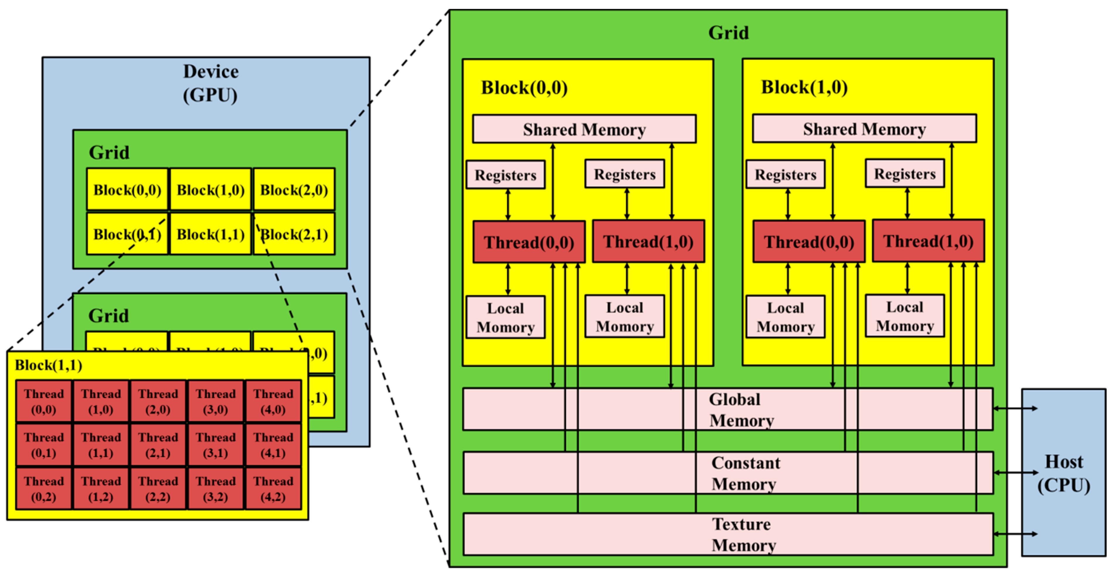
The GPU version of the diffusive wave code was implemented using CUDA Fortran, a parallel computing platform developed by NVIDIA. As shown in Figure 1, threads are grouped into block and blocks are grouped into grid in CUDA. Thus, it is convenient to associate the thread block with a particular index as follows because many applications of rainfall runoff models involve large two-dimensional data.

i = threadidx%x + (blockidx%x − 1) × blockDim%x,

(29)

j = threadidx%y + (blockidx%y − 1) × blockDim%y,

(30)

where i and j are the thread index, respectively. blockidx%x and blockidx%y are the dimensions of the block identifiers in the x and y direction, and blockDim%x and blockDim%y are the dimensions of the block dimensions, respectively.

CUDA can control several types of memory in GPU such as global, local, texture, constant, shared, and register as shown in Figure 1. Among them, register memory is the fastest variable memory and visible to thread, thus it is most advantageous to use register as much as possible. The blocks in a grid are executed independently and it is not necessary to communicate or cooperate between blocks because the numerical scheme of the diffusive wave equation does not include simultaneous equation solvers such as Gaussian elimination or Thomas algorithm, which is inherently in serial significantly increasing the running time. Therefore, very straightforward and simple implementation using mainly register memory for the diffusive wave equation was possible without using shared memory or texture.

The numerical model was implemented and tested in a PC environment with an Intel Core i7-8700K 4.70-GHz CPU, 16 GB RAM, and an NVIDIA GeForce GTX 1060 GPU with 1152 cores. In the PC system used in this study, the maximum number of threads was 1024 per block in the GPU. Thus, when we needed to simulate which array size was larger than 1024, we used multiple blocks with 1024 threads each.

3. Results and Verification

3.1. Moving Storms on 1D Impermeable Overland Plane

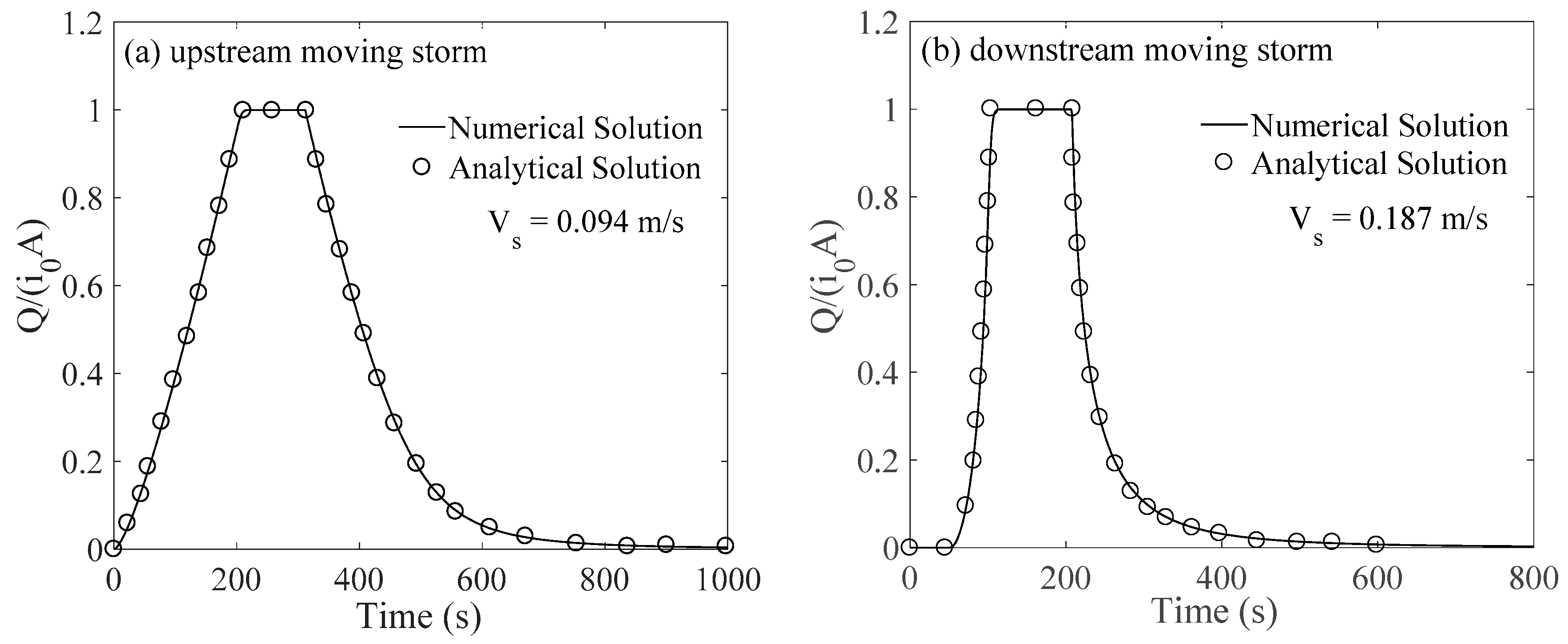
To verify the accuracy of the proposed model, we compared the computed results to the analytical solution proposed by Singh [34]. The test basin was an impermeable single overland plane. The basin length was 9.754 m with a bottom slope of 0.04 and Manning’s roughness coefficient of $n=0.04{ \mathrm{m}}^{-1/3}{\mathrm{s}}^{-1}$. The rainstorm length was 29.26 m and its rainfall intensity was i₀ = 88.9 mm/h. The storm movement speeds were $V_s=0.094 \mathrm{m}/\mathrm{s}$. and $0.187 \mathrm{m}/\mathrm{s}$ for the upstream and downstream moving cases, respectively. For the numerical simulations, the computational grid size and time step were set to $\Delta x=0.0254 \mathrm{m}$ and $\Delta t=0.01 \mathrm{s}$, respectively. A transmissive boundary condition was applied at the downstream boundary and a reflective boundary condition was applied everywhere else. Initially, a value of $h=0 \mathrm{m}$ was assumed for the entire domain. Figure 2 indicates close agreement between the relative unit discharges at the basin outlet calculated by the analytical solution and numerical model. The root-mean-square errors (RMSE) were 0.0071 and 0.043 for the upstream and downstream moving storm cases, respectively.

3.2. 1D Permeable Basin with Local Depressions

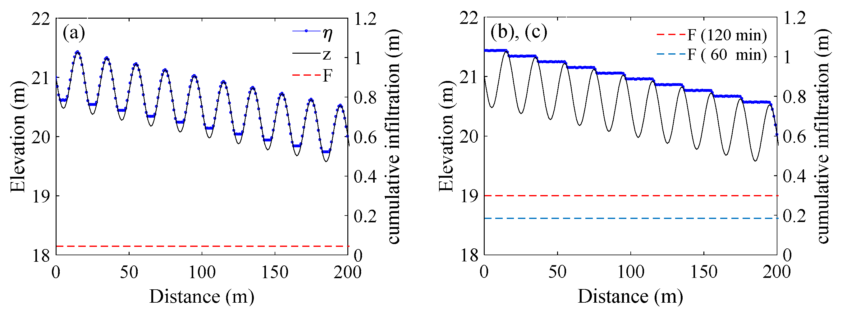
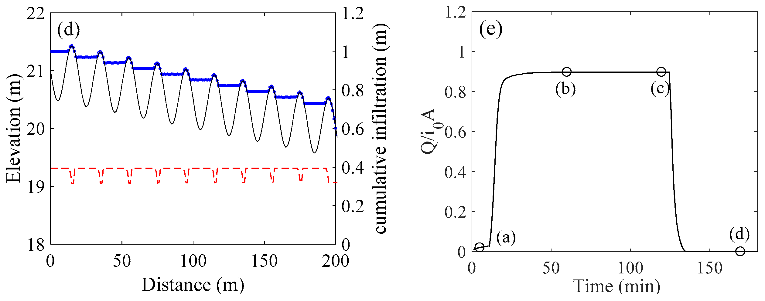
One of the most significant disadvantages of the kinematic wave models is that the flow path and direction are determined solely by the gravity, without considering other momentum factors. In other words, the signs of the slopes of the water surface profile and basin bottom profile must be the same. Therefore, if the topography of a basin has a depression, such as, a furrow or pond then, one can use kinematic wave models only after modifying the local depressive topography. In this section, the diffusive wave model is applied to an inclined sinusoidal plane (Figure 3) to test its applicability to topographies containing depressions. The bottom profile of the test basin with an inclined sinusoidal shape is defined as follows:

$$z=21.0-0.5sin\left(\frac{\pi }{10}x\right)-0.005x, 0 \mathrm{m}\le x\le 200 \mathrm{m}.$$

(31)

The initial water depth was $h=0 \mathrm{m}$ for the entire basin and a steady uniform rainfall intensity with $i_0=0.25 \mathrm{mm}/\mathrm{s}$ lasted for $125 \min .$ The infiltration rate was calculated using the Horton infiltration model with parameter values of k = $2.43 \times {10}^{-3} {\mathrm{s}}^{-1}$, $f_0 =1.977 \times {10}^{-4} \mathrm{m}/\mathrm{s}$, and $f_c =3.272 \times {10}^{-5} \mathrm{m}/\mathrm{s}$. The computational grid size was $\Delta x= \Delta y=1.0 \mathrm{m}$ and the time interval was $\Delta t=0.01 \mathrm{s}$. For the simulation, a transmissive boundary condition was applied at the downstream boundary and a reflective boundary condition was applied everywhere else. Figure 3 presents the computed profiles for water level, cumulative infiltration, and hydrograph at the basin outlet. At the beginning of the simulation, most of the rainwater was not released into the basin outlet, but flowed into the troughs by following the terrain. After rainwater filled the furrows, as shown in Figure 3b,c, the rainwater falling on the entire basin could flow toward the basin outlet, thereby increasing the discharge, as shown in Figure 3e. Since the loss through infiltration was somewhat considerable, the discharge at the basin outlet was much smaller than the equilibrium discharge. Figure 3d reveals that the water surface elevation decreased after the rain stopped by infiltration. Additionally, the cumulative infiltration became non-uniform as the dry bed area extended.

3.3. 2D Catchments

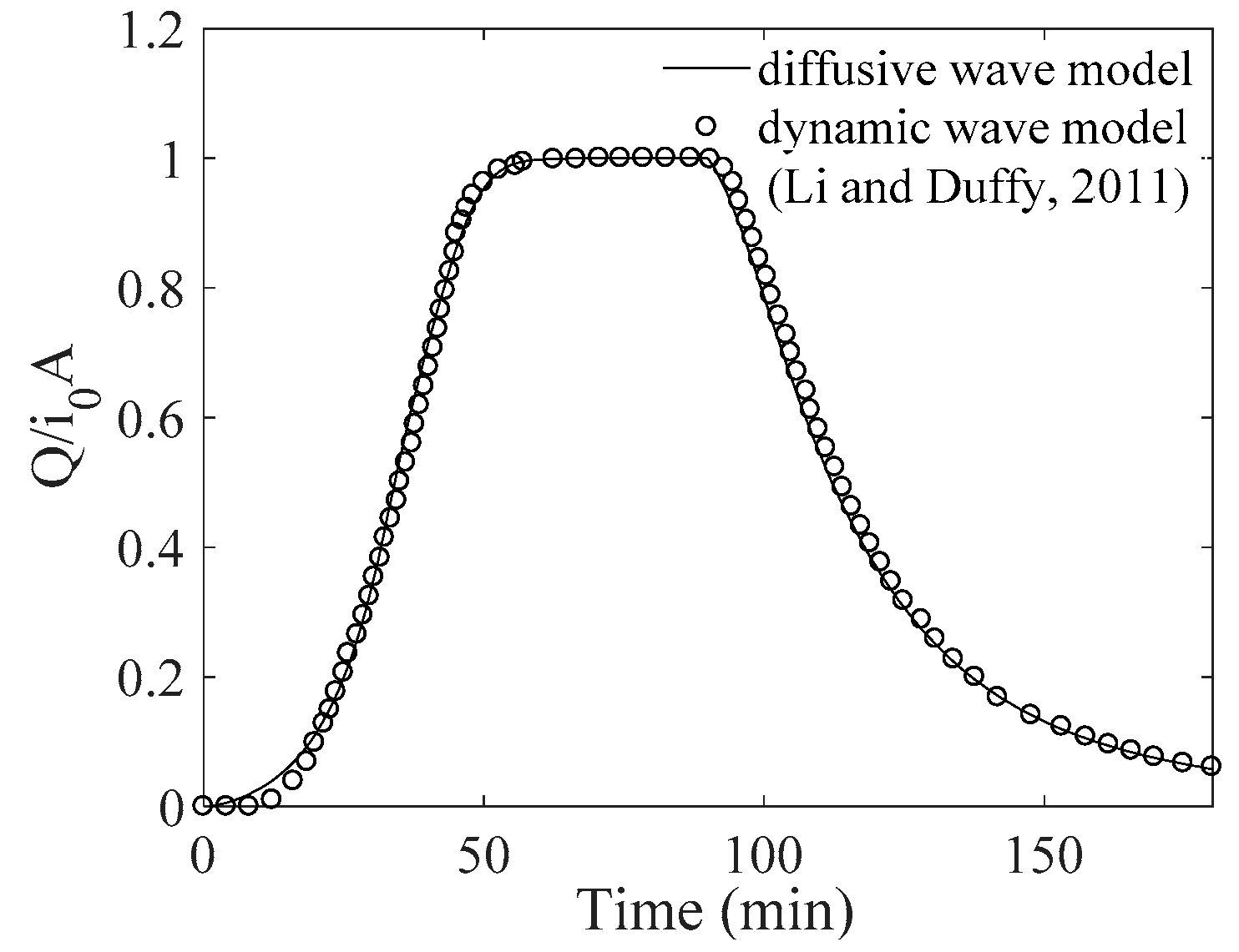
To test the applicability of the diffusive wave model to 2D spaces, we applied the model to a V-shaped basin consisting of two 1000$\mathrm{m}\times$ 800$\mathrm{m}$ planes and one 1000$\mathrm{m}\times$20$\mathrm{m}$ channel. The slope of the plane perpendicular to the channel was 0.05 and the channel bottom slope 0.02. Manning’s roughness coefficient was $n=0.015 {\mathrm{m}}^{-1/3}{\mathrm{s}}^{-1}$ for the entire domain. A constant rainfall intensity of $i_0=10.8 \mathrm{mm}/\mathrm{h}$ was uniformly applied for $90 \min$. A transmissive boundary condition was applied at the downstream boundary and a reflective boundary condition was applied on the sides and upstream boundaries. The grid sizes were $\Delta x=\Delta y=10 \mathrm{m}$ and the time step was $\Delta t=1.0 \mathrm{s}$. Figure 4 presents the discharges at the downstream boundary computed by the diffusive wave model and a dynamic wave model [35]. The RMSE normalized by the peak discharge at the outlet was 0.0263.

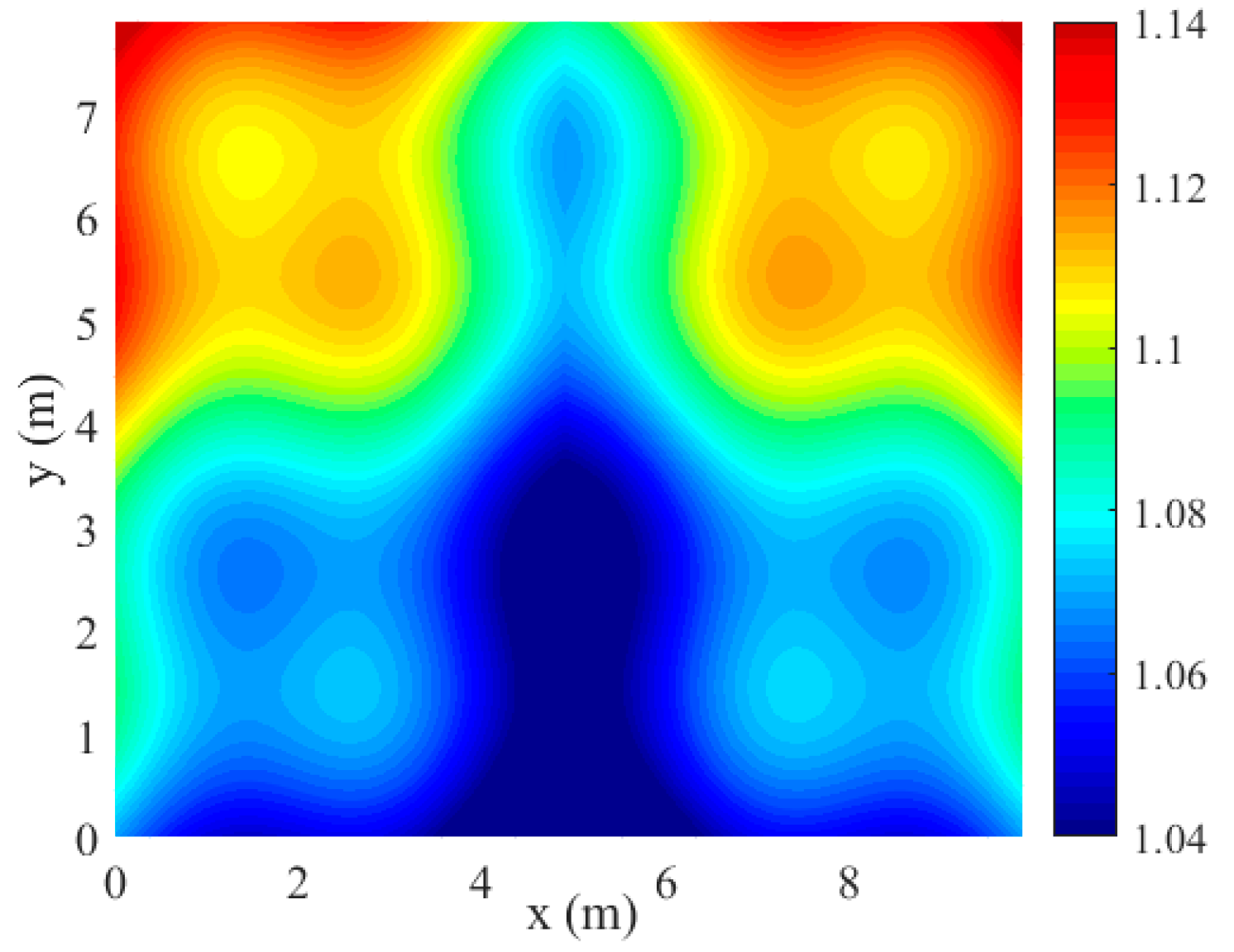
Next, the diffusive wave model was applied to a 2D basin with several storage ponds to test the model’s ability to simulating runoff processes including disconnected water bodies with depressed topography. The basin topography was defined as $z=0.01y+0.01\left|x-5\right|-0.01\sin \left(\pi x/2\right)-0.01sin\left(\pi y/2\right)+1$, where $0\le x\le 10 \mathrm{m}$ and $0\le y\le 8 \mathrm{m}$. Therefore, there were four circular ponds and a channel with two troughs, as shown in Figure 5.

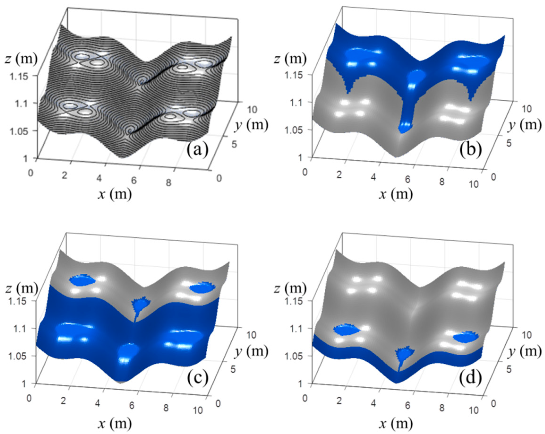
The Manning’s roughness coefficient was $n=0.013{ \mathrm{m}}^{-1/3}{\mathrm{s}}^{-1}$. The basin was permeable and the coefficients were $k=2.67 \times {10}^{-2}/\mathrm{s}$, $f_0 =7.78 \times {10}^{-5} \mathrm{m}/\mathrm{s}$, and $f_c =7.64 \times {10}^{-6} \mathrm{m}/\mathrm{s}$. A rainstorm with a speed of $0.5 \mathrm{m}/\min$ moved from the upstream side to the downstream side of the basin. Rainfall with an intensity of $i_0=50 \mathrm{mm}/\mathrm{h}$ lasted for $40 \min$. For the numerical simulation, the grid sizes were $\Delta x=\Delta y=0.1 \mathrm{m}$ and the time step was $\Delta t=0.01 \mathrm{s}$. A transmissive boundary condition was applied at the downstream boundary and a reflective boundary condition was applied at the sides and upstream boundaries. Figure 6 presents the computed results at several stages. Initially, the entire domain was dry, as shown in Figure 6a. After it began to rain, the two ponds in the upper area were filled with water and the excessive water overflowed the ponds, as shown in Figure 6b. The rainstorm continued moving in the downstream direction, so most of the upper basin area became dry, except for inside the ponds, as shown in Figure 6c. Rain still precipitated in the downstream area, meaning the lower area became flooded. Figure 6d reveals that the water in the two ponds in the upper area disappeared through infiltration. From this figure, one can see that the diffusive wave model reproduced physically reasonable rainfall runoff processes on a complex topography with 2D depressions. Considering the results of these two test cases, the proposed diffusive wave model is a promising prediction tool for rainfall runoff processes in 2D catchments.

3.4. Complex Natural Basin

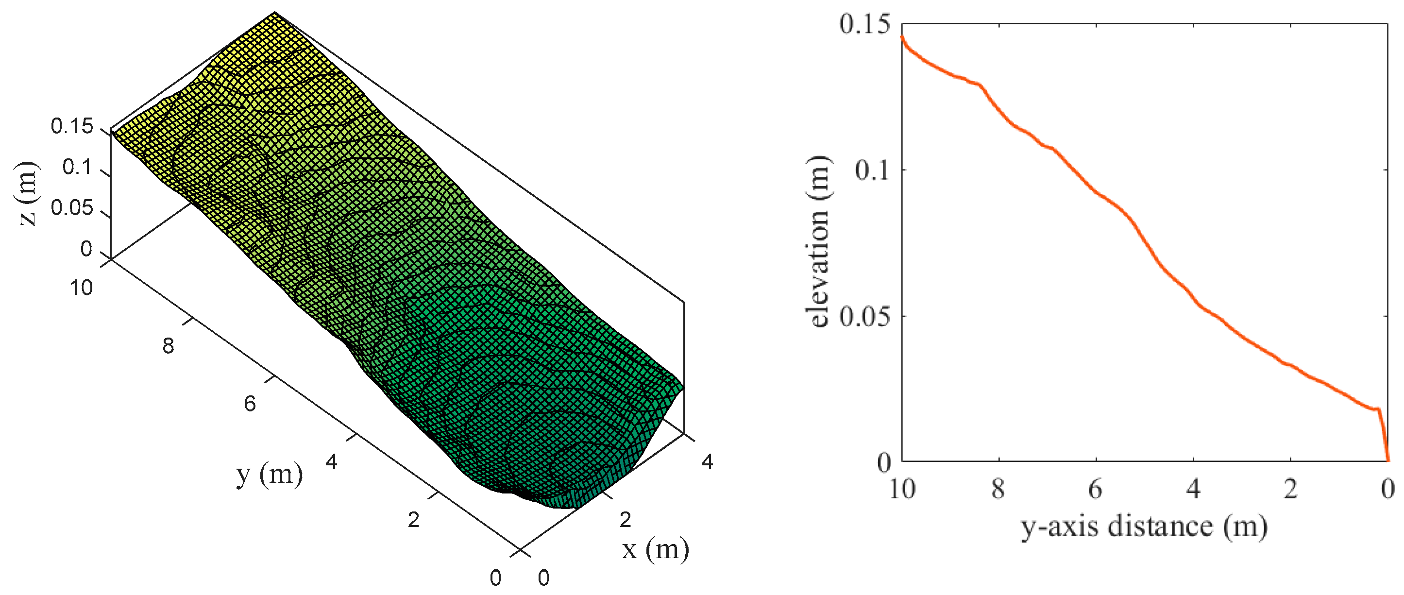
The diffusive wave model was tested on a real catchment and the results were compared to measured data. The domain was 10 m long and 4 m wide with an average bottom slope of 0.01, as shown in Figure 7. Prior to the experiment, rainfall continued for several hours, meaning the soil erosion effect was sufficiently slow to ignore the bottom evolution that occurred during the experiment. For the numerical simulation, the $10 \times 10 {\mathrm{cm}}^2$ digital elevation model (DEM) presented by Tartard et al. [36] with parameters of $\Delta t=0.01 \mathrm{s}$ and $i_0=70 \mathrm{mm}/\mathrm{h}$ was used. A transmissive boundary condition was also applied at the downstream boundary and a reflective boundary condition was applied to other boundaries.

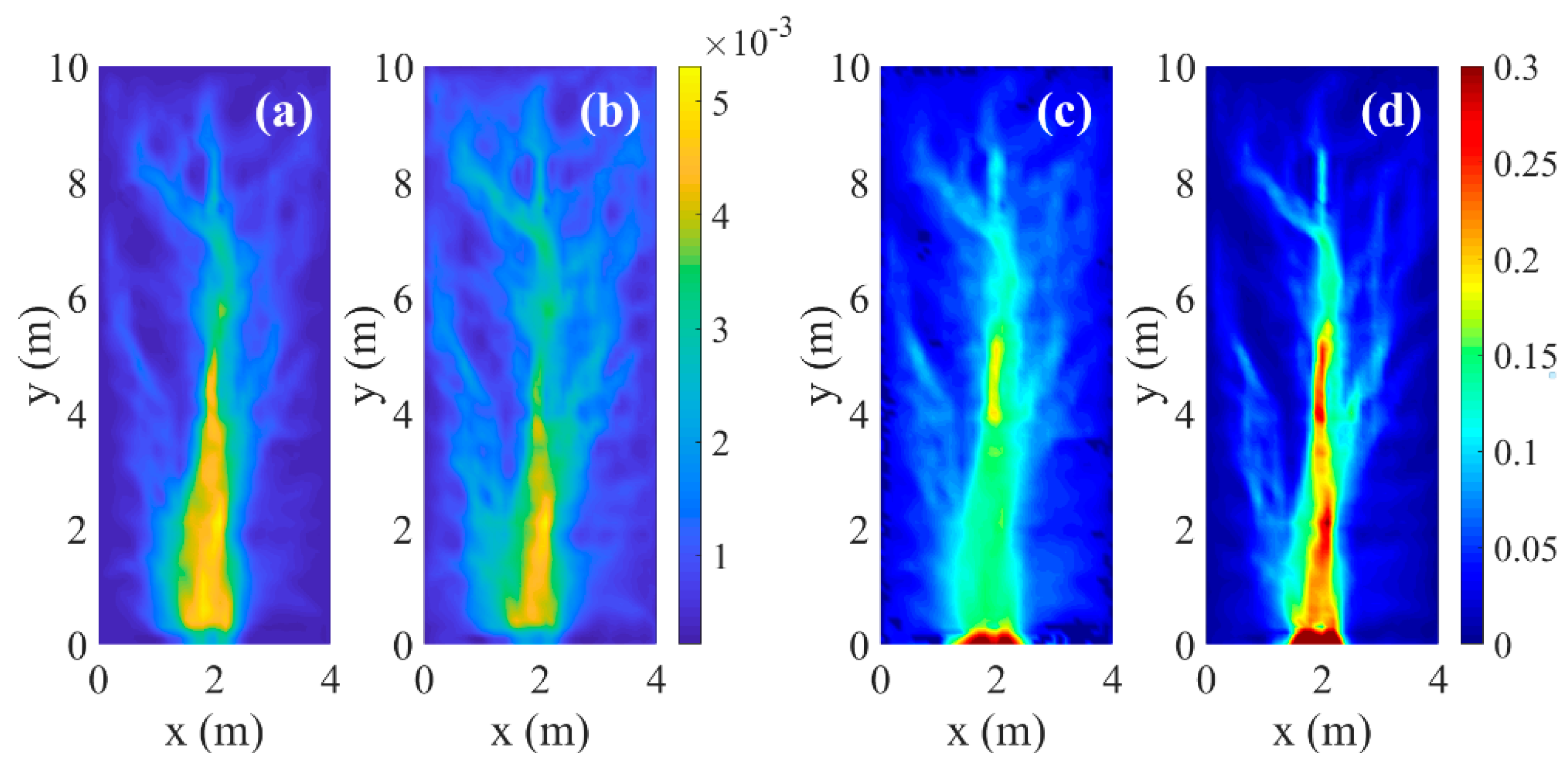
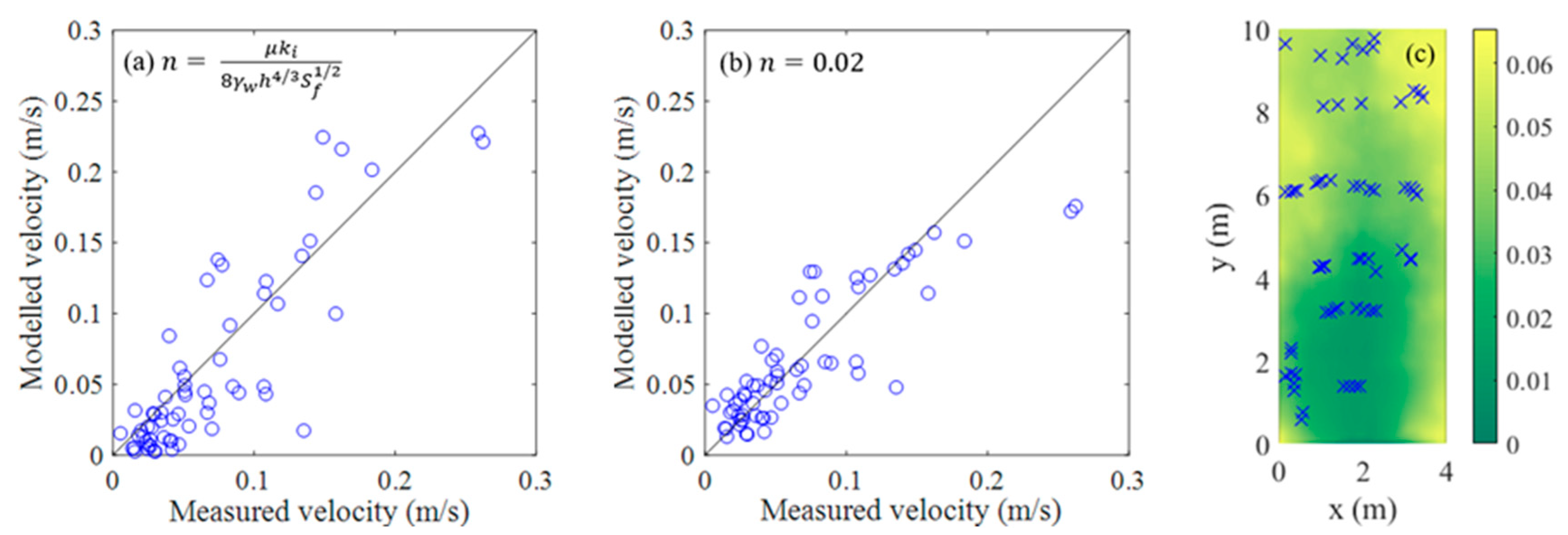
Figure 8 presents the complex dendritic patterns of the computed water depth and flow velocity generated by following the complex terrain. Both plots of computed flow velocity show a rapid increase in the flow velocity in downstream area corresponding to the relative steep bottom slope. Figure 9 presents a comparison between the computed velocity of the proposed model and the measured velocity [36,37] at the 62 points. The RMSEs of the computed results were 0.0284 $\mathrm{m}/\mathrm{s}$ and 0.0343 $\mathrm{m}/\mathrm{s}$ when using $n=0.02$ and when using Equation (16), respectively. For reference, Mugler et al. [38] obtained an RMSE of 0.03 $\mathrm{m}/\mathrm{s}$ for the same case using a diffusive wave model. One of the main reasons for discrepancy is that the computed velocities were averaged over a $10 \times 10{ \mathrm{cm}}^2$ area, while the measured velocities [36,37] were based on points. Additionally, the low spatial resolution of the topography and exclusion of local and advective accelerations from the momentum equation may lead to small errors.

4. GPU Speedup of Parallel Computing

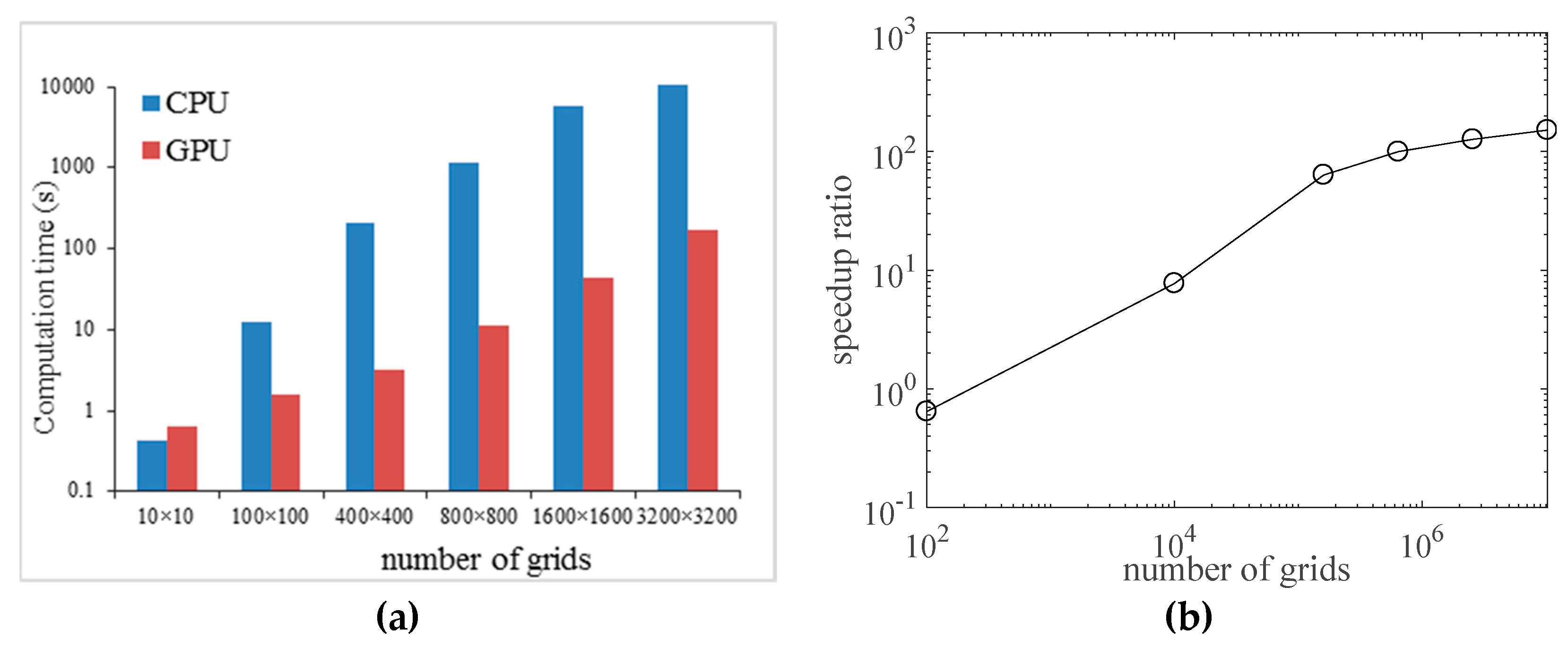
In this section, we compared the performance of the GPU-accelerated diffusive wave model using an NVIDIA GeForce GTX 1060 GPU with 1152 cores to that of the CPU version using an Intel i7 4.7-GHz CPU in a PC environment. To compare the two versions, we simulated the V-shaped basin case from Section 3.3 with various numbers of grids ranging from ${10}^2$ to $1.024 \times {10}^7$. Also, the numerical test was performed for only one minute because the purpose was to compare the computation times of the GPU and CPU versions. Figure 10 presents the computation times of the GPU and CPU versions, as well as the speedup ratio achieved by parallel computing, where the speedup ratio is defined as the ratio of the computation times of the GPU and CPU versions. When the number of the grids was $10 \times 10$, the speedup ratio was less than one because there is a time delay associated with transferring data between the CPU and GPU. However, the GPU-accelerated version became much more efficient than the CPU version as the number of grids increased. For the grid number of $3200 \times 3200$, the GPU version finished computation approximately 150 times faster than the CPU version.

5. Conclusions

In this study, we developed and tested a GPU-accelerated 2D diffusive wave model for simulating rainfall runoff processes. The diffusive wave equations were solved using a Godunov-type finite volume scheme. The flux at the computational cell interface was reconstructed using piecewise linear MUSCL with a van Leer slope TVD limiter. Infiltration was computed using the Horton infiltration model. Parallelization was implemented using CUDA-Fortran in a PC environment with an NVIDIA GeForce GTX 1060 GPU. The proposed model was first applied to 1D and 2D impermeable basins without depressions. The computed results were compared to analytical solutions and the dynamic wave model results showed very close agreement with the analytical solutions. We then applied the diffusive wave model to 1D and 2D permeable basins with depressions, such as furrows or ponds. The diffusive wave model reasonably simulated the overland flow around the depressions. Finally, we applied the diffusive wave model to a real basin with complex terrain and reasonable agreement with the measured data was observed. The performance of parallel computing became very efficient as the number of the computational grids increased, achieving a maximum speedup ratio of approximately 150 times compared to the CPU version using an Intel i7 CPU in a PC environment.

Although we proposed a GPU-accelerated high resolution numerical scheme for diffusive wave equations, it is necessary to integrate with various hydrological processes modules such as river flow, groundwater, vegetation effect, and hydraulic structure for practical application of the model to real watersheds, which are beyond this study. Since the width of streams varies from centimeter to kilometer scales, the present grid based rainfall runoff model cannot properly describe river geometry. Rainfall runoff is also significantly affected by groundwater flow and hydraulic structure, which require many parameters such as hydraulic conductivity, porosity, and operation rules.

References

- Beven, K.J. Rainfall-Runoff Modelling: The Primer; Wiley-Blackwell: Hoboken, NJ, USA, 2012; ISBN 9780470714591. [Google Scholar]
- Uhlenbrook, S.; Seibert, J.A.N.; Leibundgut, C.; Rodhe, A. Prediction uncertainty of conceptual rainfall-runoff models caused by problems in identifying model parameters and structure. Hydrol. Sci. J. 1999, 44, 779–797. [Google Scholar] [CrossRef]
- Zhou, J.G.; Causon, D.M.; Mingham, C.G.; Ingram, D.M. The surface gradient method for the treatment of source terms in the shallow-water equations. J. Comput. Phys. 2001, 168, 1–25. [Google Scholar] [CrossRef]
- Mignot, E.; Paquier, A.; Haider, S. Modeling floods in a dense urban area using 2D shallow water equations. J. Hydrol. 2006, 327, 186–199. [Google Scholar] [CrossRef] [Green Version]
- Ajayi, A.E.; van de Giesen, N.; Vlek, P. A numerical model for simulating Hortonian overland flow on tropical hillslopes with vegetation elements. Hydrol. Process. 2008, 22, 1107–1118. [Google Scholar] [CrossRef]
- Yeh, G.T.; Shih, D.S.; Cheng, J.R.C. An integrated media, integrated processes watershed model. Comput. Fluid. 2011, 45, 2–13. [Google Scholar] [CrossRef]
- Costabile, P.; Costanzo, C.; Macchione, F. Comparative analysis of overland flow models using finite volume schemes. J. Hydroinform. 2012, 14, 122–135. [Google Scholar] [CrossRef]
- Costabile, P.; Costanzo, C.; Macchione, F. A storm event watershed model for surface runoff based on 2D fully dynamic wave equations. Hydrol. Process. 2012, 27, 554–569. [Google Scholar] [CrossRef]
- Caviedes-Voullième, D.; García-Navarro, P.; Murillo, J. Influence of mesh structure on 2D full shallow water equations and SCS Curve Number simulation of rainfall/runoff events. J. Hydrol. 2012, 448, 39–59. [Google Scholar]
- Kim, J.; Warnock, A.; Ivanov, V.Y.; Katopodes, N.D. Coupled modeling of hydrologic and hydrodynamic processes including overland and channel flow. Adv. Water Resour. 2012, 37, 104–126. [Google Scholar] [CrossRef]
- Kim, D.H.; Seo, Y. Hydrodynamic analysis of storm movement effects on runoff hydrographs and loop-rating curves of a V-shaped watershed. Water Resour. Res. 2013, 49, 6613–6623. [Google Scholar] [CrossRef]
- Fernández-Pato, J.; Caviedes-Voullième, D.; García-Navarro, P. Rainfall/runoff simulation with 2D full shallow water equations: Sensitivity analysis and calibration of infiltration parameters. J. Hydrol. 2016, 536, 496–513. [Google Scholar] [CrossRef]
- Lighthill, M.J.; Whitham, G.B. On kinematic waves I. Flood movement in long rivers. Proc. R. Soc. Lond. A Math. Phys. Sci. 1955, 229, 281–316. [Google Scholar]
- Ponce, V.M. Engineering Hydrology: Principles and Practices; Prentice Hall: Hoboken, NJ, USA, 1994; ISBN 9780133154665. [Google Scholar]
- Liu, Q.Q.; Chen, L.; Li, J.C.; Singh, V.P. Two-dimensional kinematic wave model of overland-flow. J. Hydrol. 2004, 291, 28–41. [Google Scholar] [CrossRef]
- Singh, V.P. Kinematic wave modelling in water resources: A historical perspective. Hydrol. Process. 2001, 15, 671–706. [Google Scholar] [CrossRef]
- Yu, C.; Duan, J.G. High resolution numerical schemes for solving kinematic wave equation. J. Hydrol. 2014, 519, 823–832. [Google Scholar] [CrossRef]
- Moussa, R.; Bocquillon, C. Criteria for the choice of flood-routing methods in natural channels. J. Hydrol. 1996, 186, 1–30. [Google Scholar] [CrossRef]
- Te Chow, V. Open-Channel Hydraulics; McGraw-Hill: New York, NY, USA, 1959; ISBN 9780070107762. [Google Scholar]
- Lacasta, A.; Morales-Hernández, M.; Murillo, J.; García-Navarro, P. GPU implementation of the 2D shallow water equations for the simulation of rainfall/runoff events. Environ. Earth Sci. 2015, 74, 7295–7305. [Google Scholar] [CrossRef]
- Sitanggang, K.I.; Lynett, P. Parallel computation of a highly nonlinear Boussinesq equation model through domain decomposition. Int. J. Numer. Methods Fluids 2005, 49, 57–74. [Google Scholar] [CrossRef]
- Cordier, S.; Coullon, H.; Delestre, O.; Laguerre, C.; Le, M.H.; Pierre, D.; Sadaka, G. FullSWOF Paral: Comparison of two parallelization strategies (MPI and SKELGIS) on a software designed for hydrology applications. ESAIM Proc. 2013, 43, 59–79. [Google Scholar] [CrossRef]
- Mallón, D.A.; Taboada, G.L.; Teijeiro, C.; Tourino, J.; Fraguela, B.B.; Gómez, A.; Doallo, R.; Mourino, J.C. Performance evaluation of MPI, UPC and OpenMP on multicore architectures. In Proceedings of the 16th European PVM/MPI Users’ Group Meeting, Espoo, Finland, 7–10 September 2009; Springer: Berlin/Heidelberg, Germany, 2009; pp. 174–184. [Google Scholar]
- Neal, J.; Fewtrell, T.; Trigg, M. Parallelisation of storage cell flood models using OpenMP. Environ. Model. Softw. 2009, 24, 872–877. [Google Scholar] [CrossRef]
- Leandro, J.; Chen, A.S.; Schumann, A. A 2D parallel diffusive wave model for floodplain inundation with variable time step (P-DWave). J. Hydrol. 2014, 517, 250–259. [Google Scholar] [CrossRef]
- Kazezyılmaz-Alhan, C.M.; Medina, M.A., Jr. Kinematic and diffusion waves: Analytical and numerical solutions to overland and channel flow. J. Hydraul. Eng. 2007, 133, 217–228. [Google Scholar] [CrossRef]
- Yen, B.C.; Chow, V.T. A laboratory study of surface runoff due to moving rainstorms. Water Resour. Res. 1969, 5, 989–1006. [Google Scholar] [CrossRef]
- Woo, D.C.; Brater, E.F. Spatially varied flow from controlled rainfall. J. Hydraulics. Eng. Div. 1962, 88, 31–56. [Google Scholar]
- Yu, Y.S.; McNown, J.S. Runoff from impervious surfaces. J. Hydraul. Res. 1964, 2, 3–24. [Google Scholar] [CrossRef]
- Julien, P.Y. River Mechanics; Cambridge University Press: Cambridge, UK, 2002; ISBN 9780521529709. [Google Scholar]
- Horton, R.E. Analysis of runoff-plat experiments with varying infiltration-capacity. Eos Trans. Am. Geophys. Union 1939, 20, 693–711. [Google Scholar] [CrossRef]
- Van Leer, B. Towards the ultimate conservative difference scheme. V. A second-order sequel to Godunov’s method. J. Comput. Phys. 1979, 32, 101–136. [Google Scholar] [CrossRef]
- Mahdavi, A.; Talebbeydokhti, N. Modeling of non-breaking and breaking solitary wave run-up using FORCE-MUSCL scheme. J. Hydraul. Res. 2009, 47, 476–485. [Google Scholar] [CrossRef]
- Singh, V.P. Effect of the direction of storm movement on planar flow. Hydrol. Process. 1998, 12, 147–170. [Google Scholar] [CrossRef]
- Li, S.; Duffy, C.J. Fully coupled approach to modeling shallow water flow, sediment transport, and bed evolution in rivers. Water. Resour. Res. 2011, 47. [Google Scholar] [CrossRef]
- Tatard, L.; Planchon, O.; Wainwright, J.; Nord, G.; Favis-Mortlock, D.; Silvera, N.; Ribolzi, O.; Esteves, M.; Huang, C.H. Measurement and modelling of high-resolution flow-velocity data under simulated rainfall on a low-slope sandy soil. J. Hydrol. 2008, 348, 1–12. [Google Scholar] [CrossRef] [Green Version]
- Esteves, M.; Planchon, O.; Lapetite, J.M.; Silvera, N.; Cadet, P. The ‘EMIRE’ large rainfall simulator: Design and field testing. Earth Surf. Process. Landf. 2000, 25, 681–690. [Google Scholar] [CrossRef]
- Mügler, C.; Planchon, O.; Patin, J.; Weill, S.; Silvera, N.; Richard, P.; Mouche, E. Comparison of roughness models to simulate overland flow and tracer transport experiments under simulated rainfall at plot scale. J. Hydrol. 2011, 402, 25–40. [Google Scholar] [CrossRef]
Figure 1.
Schematic of CUDA memory hierarchy in GPU.
Figure 2.
Comparisons of computed results and analytical solutions [34]. : Basin area.
Figure 3.
(a–d) Computed water surface profile and accumulated infiltration at (a) t = 5 min, (b) t = 60 min, (c) t = 120 min, and (d) t = 170 min. (e) Hydrographs at the downstream boundary.
Figure 4.
Computed discharges at the basin outlet.
Figure 5.
Bottom elevation of a 2D test with several storage ponds.
Figure 6.
Computed water surface (blue) at (a) , (b) , (c) , (d) , and basin topography.
Figure 7.
(Left) Elevation of the tested basin in Thies, Senegal. (Right) Bottom profile along -axis at = 2 m.
Figure 8.
Computed water depths (m) using (a) n = 0.02 and (b) Equation (16). Computed flow velocity (m/s) using (c) n = 0.02 and (d) Equation (16).
Figure 9.
(a,b) Comparison between the computed velocity and measured velocity [36,37]. (c) Locations of measured points and bottom elevation of the tested basin.
Figure 10.
Performance comparison between the GPU and CPU models through (a) computation time (s), (b) speedup ratio.
© 2019 by the authors. Licensee MDPI, Basel, Switzerland. This article is an open access article distributed under the terms and conditions of the Creative Commons Attribution (CC BY) license (http://creativecommons.org/licenses/by/4.0/).
Share and Cite
MDPI and ACS Style
Park, S.; Kim, B.; Kim, D.-H. 2D GPU-Accelerated High Resolution Numerical Scheme for Solving Diffusive Wave Equations. Water 2019, 11, 1447. https://doi.org/10.3390/w11071447
AMA Style
Park S, Kim B, Kim D-H. 2D GPU-Accelerated High Resolution Numerical Scheme for Solving Diffusive Wave Equations. Water. 2019; 11(7):1447. https://doi.org/10.3390/w11071447
Chicago/Turabian StylePark, Seonryang, Boram Kim, and Dae-Hong Kim. 2019. "2D GPU-Accelerated High Resolution Numerical Scheme for Solving Diffusive Wave Equations" Water 11, no. 7: 1447. https://doi.org/10.3390/w11071447
Note that from the first issue of 2016, this journal uses article numbers instead of page numbers. See further details here.