A Case Study: Response Mechanics of Irregular Rotational Tidal Flows to Outlet Regulation in Yangtze Estuary


1
School of Hydropower and Information Engineering, Huazhong University of Science and Technology, Wuhan 430074, China
2
Yangtze River Scientific Research Institute, Wuhan 430010, China
*
Author to whom correspondence should be addressed.
Water 2019, 11(7), 1445; https://doi.org/10.3390/w11071445
Submission received: 7 July 2019
/
Revised: 10 July 2019
/
Accepted: 11 July 2019
/
Published: 12 July 2019
(This article belongs to the Section Water Quality and Contamination)
Abstract
:Responses of irregular rotational tidal flows to an outlet regulation (the Guyuan Sand (GYS) regulation) in the three-level branching Yangtze Estuary are studied by a high-resolution numerical model and theoretical analysis. The project is launched around GYS at the outlet of the North Branch of the Yangtze Estuary. The tidal flows around GYS are rotational and become irregular under the influences of the runoff-tide interactions, rapidly varying topographies and complex solid boundaries in coastal areas. Three designs of GYS regulation were studied, including various diversion dikes and new outlets of different widths. The regulation disturbs the irregular rotational flows around GYS, and further changes the estuarine tidal processes and the water exchange between different branches of the branching Yangtze Estuary. It was interesting to find that additional current and additional storage are formed along the North Branch when a southward outlet and the clockwise rotational flow met around GYS. This special phenomenon is named “guide effect” in this study. The guide effect, together with common resist effect (arising from the narrowed outlet channel), reshapes the estuarine tidal processes. Based on the simulation result and a theoretical analysis, response mechanics of irregular rotational tidal flows to the outlet regulation in complex branching estuaries are quantitatively studied.
1. Introduction
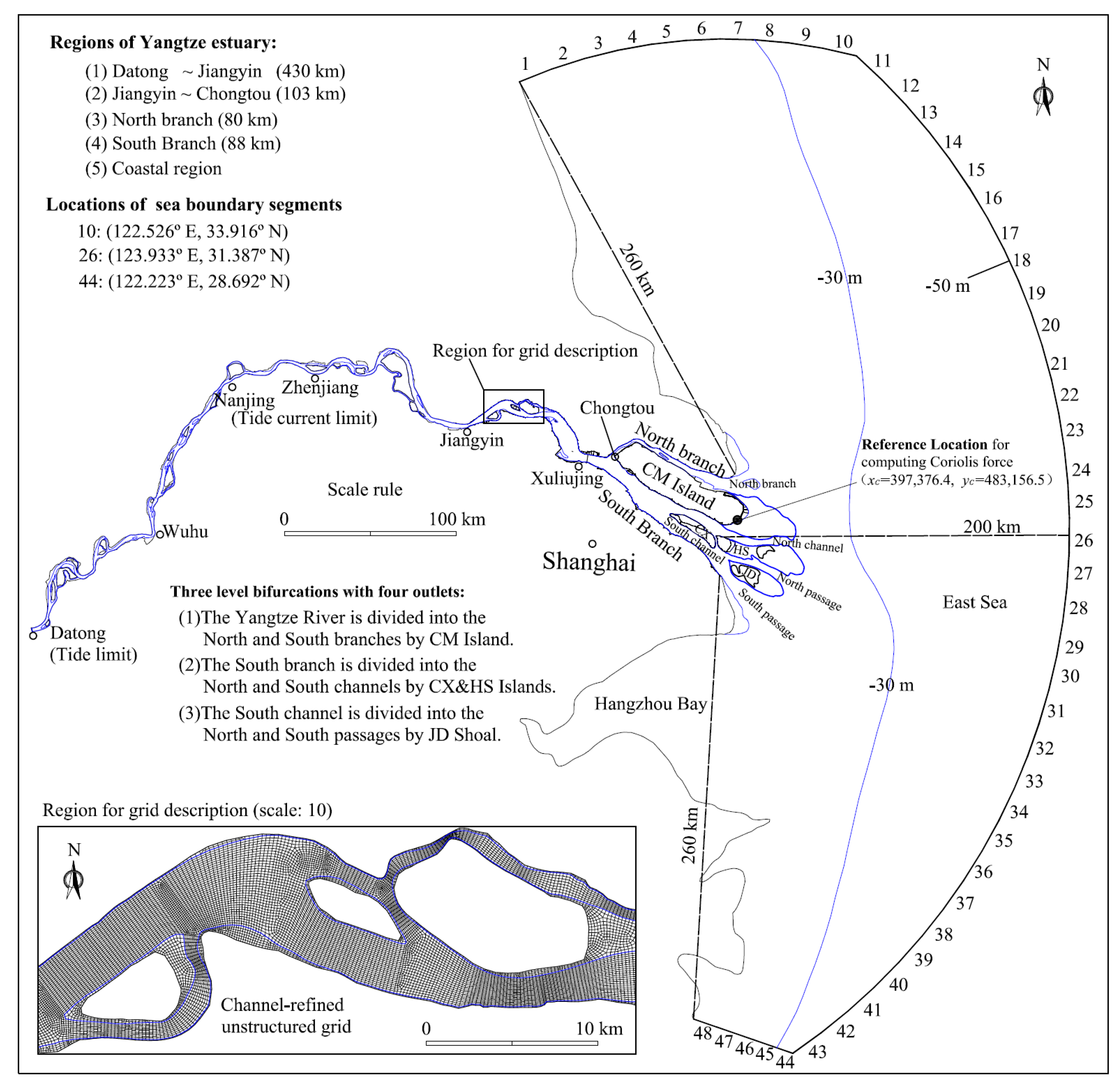
The Yangtze Estuary is a large-scale shallow water system characterized by three-level bifurcations (North and South Branches, North and South Channels, North and South Passages) and has four outlets into the East Sea, as shown in Figure 1. Significant runoffs from the Yangtze River (about 9000 × 108 m3/year) and periodical tides from the ocean meet in the estuary and interact with each other, leading to complicated hydrodynamics. Moreover, as a famous phenomenon of the branching Yangtze Estuary, landward flood-tide flows are often observed to spill over from the North to the South Branch [1]. Surrounded by the most developed regions of China (Shanghai city and Jiangsu Province), the Yangtze Estuary has seen extensive launching of various projects such as reclamations and regulations [2,3,4,5], reservoirs [6] and navigation regulations [7,8,9,10,11] because of the requirements for the developments of cities.
The North Branch of the Yangtze Estuary is characterized by a special morphology [1]. The upper reach is narrow and almost orthogonal to the South Branch, preventing upstream inflows from entering during ebb tides. The lower and tail reaches are trumpet-shaped with a wide outlet, in favor of accommodating a great deal of landward tidal flows during flood tides. Because of such special morphology, the cities along the North Branch of the estuary often suffer serious flood threat under extreme weather. To improve the morphology of the North Branch and reduce the flood risk of the neighboring cities, the Chinese government planned to build new outlet channels for the North Branch around the Guyuan Sand (GYS). The GYS regulation may lead to complex disturbance of the tidal flows in the Yangtze Estuary, which are analyzed as follows.
First, the GYS is located just outside of one outlet (of the North Branch) of the Yangtze Estuary, where bidirectional flows inside the estuary evolve gradually into clockwise rotational tidal flows in offshore regions. Tidal flows around the GYS are shown to be rotational and irregular, under the influence of runoff-tide interactions, rapidly varying topographies and complex solid boundaries in coastal areas. Correspondingly, responses of the irregular rotational flows to the redirected outlet channels in the GYS regulation are complex. Second, the river, the coast, and the ocean in the Yangtze Estuary are closely related. The tidal processes, not only in the coastal areas but also in the upstream tidal reaches and downstream offshore regions, are all disturbed by the GYS regulation. Third, in a branching estuary such as the Yangtze Estuary, the GYS regulation will also change the exchange of water between different branches. To figure out the complex influences of the GYS regulation on the tidal flows of the branching Yangtze Estuary is therefore challenging.
In this paper, a high-resolution two-dimensional (2D) hydrodynamic model is developed to simulate the irregular rotational tidal flows with and without the GYS regulation in the Yangtze Estuary, where response mechanics of the flows to the regulation is clarified.
2. Numerical Model for Yangtze Estuary
2.1. Numerical Formulation
Depth-averaged 2D shallow water equations (SWEs), with Coriolis terms, are used as the governing equations for the hydrodynamic model, which are given by
where h(x, y, t) is the water depth, (m); u(x, y, t) and v(x, y, t) are the components of vertically averaged velocity in the horizontal x- and y-directions, respectively, (m/s); t is the time, (s); g is the gravitational acceleration, (m/s2); η(x, y, t) is the water level measured from an undisturbed reference water surface, (m); υt is the coefficient of the horizontal eddy viscosity, (m2/s); f is Coriolis factor; nm is Manning’s roughness coefficient, (m−1/3 s); ρ is the water density, (kg/m3); and τsx and τsy are the wind stress in the x- and y-directions, respectively, (N/m2).
The above equations construct a set of equations for u, v and η. Their forms are invariable in the rotating frame of unstructured grids. The wind stress is imposed as per References [12,13]. For a given location (x, y) of the Yangtze Estuary, the Coriolis factor f is given by
where Ω (=7.29 × 10⁻⁵ rad/s) is the angular velocity of rotation of the Earth; ϕ (=31.38724°) is the latitude of the reference location (xc, yc) which is shown in Figure 2.
The adopted hydrodynamic model [14,15,16,17] uses a θ semi-implicit formulation [18], while the finite-volume and finite-difference methods are combined. Momentum equations are solved within a finite-difference framework and using operator-splitting techniques. The θ semi-implicit method is used to advance the time stepping. Correspondingly, the gradient of the free-surface elevation is discretized into explicit and implicit parts. A point-wise Eulerian–Lagrangian method (ELM), using the multistep backward Euler technique [19,20], is used to solve the advection term. The horizontal diffusion term is discretized using an explicit center-difference method. The finite-volume method is used for cell update of the continuity equation. The resulting flow model is mass-conservative and allows large time steps for which the Courant number could be greater than 1.
2.2. Computational Grid and Boundary Conditions
To get a full description of the river–coast–ocean coupling, the upstream tidal reach, the entire Yangtze Estuary and partial East Sea are included in a single model. Station Datong (620 km upstream of the outlets), which is regarded as the tidal limit of the estuary and has routinely hydrological field data, was chosen as the upstream boundary. Seaward open boundaries are extended to deep-water (>50 m) regions, where a global tide model (GTM) [21] can provide an accurate history of astronomical tides. The eastern seaward open boundary is located around 124° E, with southern and northern boundaries being at 28.7° N and 33.9° N, respectively.
With three-level bifurcations and tens of islands or shoals, the Yangtze Estuary has complex river regimes [22]. The common resolution of bathymetry graphs, for an accurate description of the local river regimes of the Yangtze Estuary, is listed in Table 1. Coarse computational grids only describe an oversmoothed riverbed and are unable to correctly solve estuarine mesoscale structures [23] and transport process [24]. To ensure a good description of irregular boundaries and local river regimes, a channel-refined unstructured grid, whose grid scale (listed in Table 1) is approximately equal to the intervals between two neighboring survey points of the corresponding bathymetry graph, is used. The main-flow channels in tidal reaches are covered by refined structured-like grids, with floodplains and inner islands covered by relatively coarse unstructured grids. There are 199,310 quad cells, and an example of the grid is given in Figure 2 (see Figure S1 for details).
Field data of discharges at Station Datong were used to set the upstream boundary conditions. The seaward open boundary is forced by semidiurnal tides. The time series of the tidal levels at the seaward boundary are predicted by the GTM developed in Reference [21]. The seaward boundary is divided into 48 segments (see Figure 2), for each of which the tidal harmonic constants are interpolated from a constituent database on a full global grid.
2.3. Calibration and Validation Tests
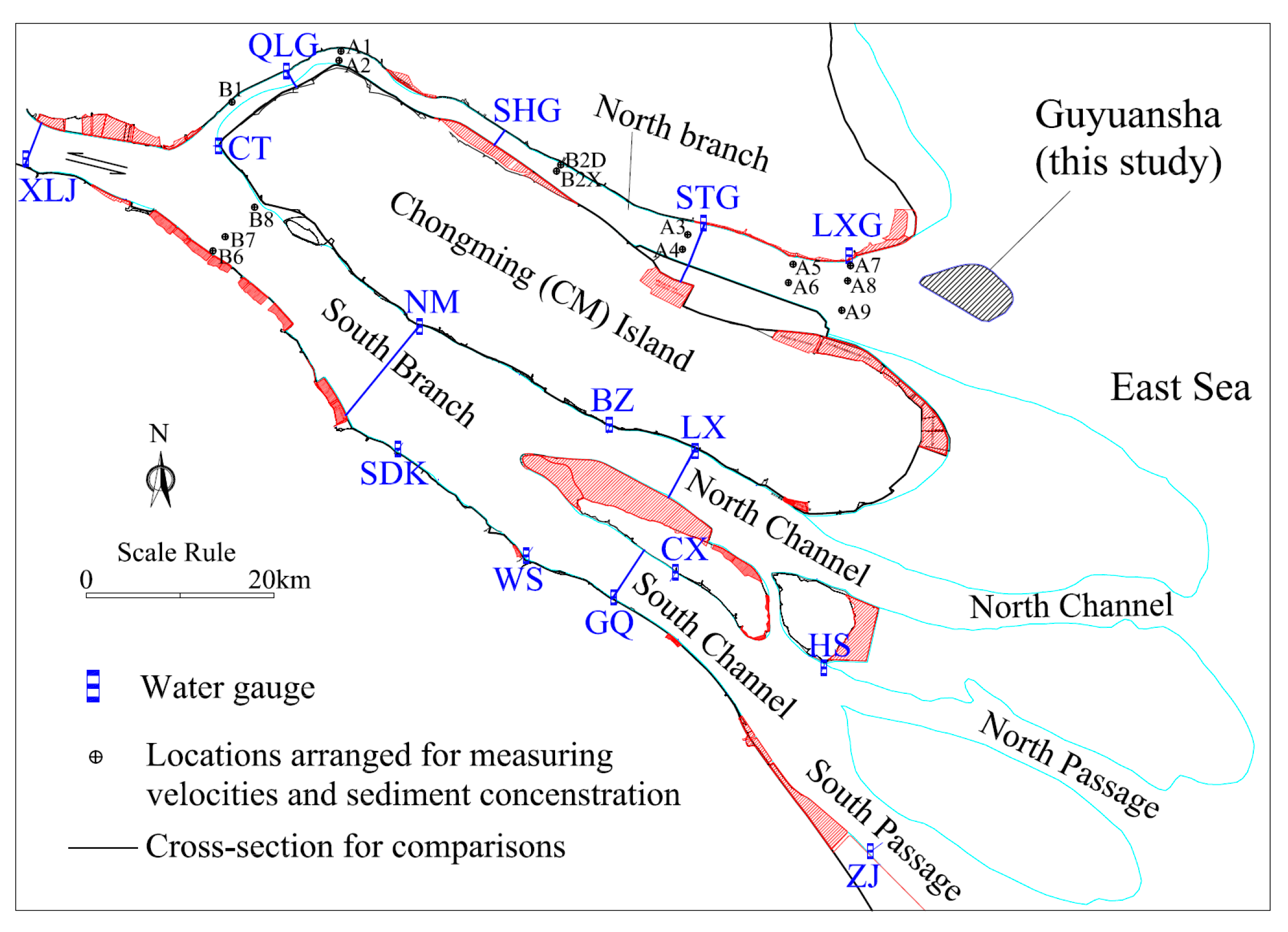
Field data of spring-neap tides during 6–16 December 2012 were used to calibrate parameters of the model and then validate its accuracy. In the hydrological survey, tidal levels were recorded at 14 fixed gauges from 6 December (the 340th day of 2012) to 16 December. The depth-averaged horizontal velocity was recorded from 8 December at 12:00 to 9 December at 21:00 for neap tides and from 14 December at 7:00 to 15 December at 13:00 for spring tides. Arrangements of the hydrological survey locations are shown in Figure 3. At the upstream boundary, the daily average river discharge at Station Datong gradually reduced from 22,000 to 18,700 m3/s during 6–16 December 2012.
In the simulations, the time step of the hydrodynamic model is set to 90 s, while nine sub steps are used in the backtracking of the ELM. For a simulation of free-surface flows, the initial condition has a significant effect on the simulation of unsteady flows. In our simulations, the initial condition was determined by a preliminary simulation, whose steps are as follows.
Manning’s roughness coefficient, nm, was calibrated using the spring-tide condition from 14 December at 0:00 to 16 December at 0:00. The inflow discharge was set to 19,000 m3/s. The nm of sub regions was adjusted so that the simulated tide-level histories would agree with field data. The nm was then corrected slightly so that the simulated velocity histories would agree with field data at the same time. The nm was finally calibrated as 0.022–0.021 from Station Datong to Jiangyin, 0.021–0.015 from Station Jiangyin to Xuliujing, and 0.014–0.011 for the North and South Branches. The nm in the North and South Branches was similar to the values reported in previous research [25,26].
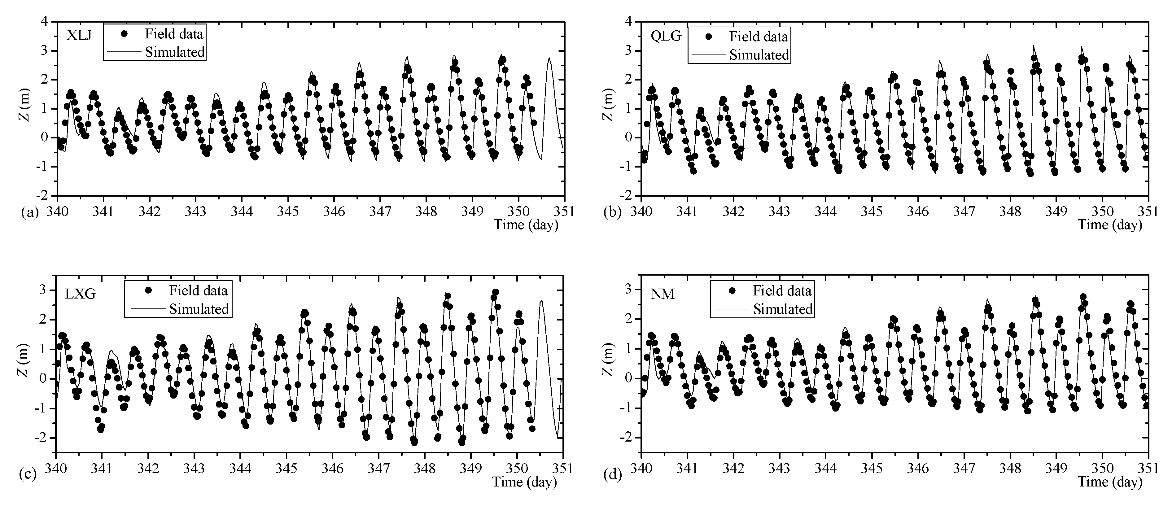
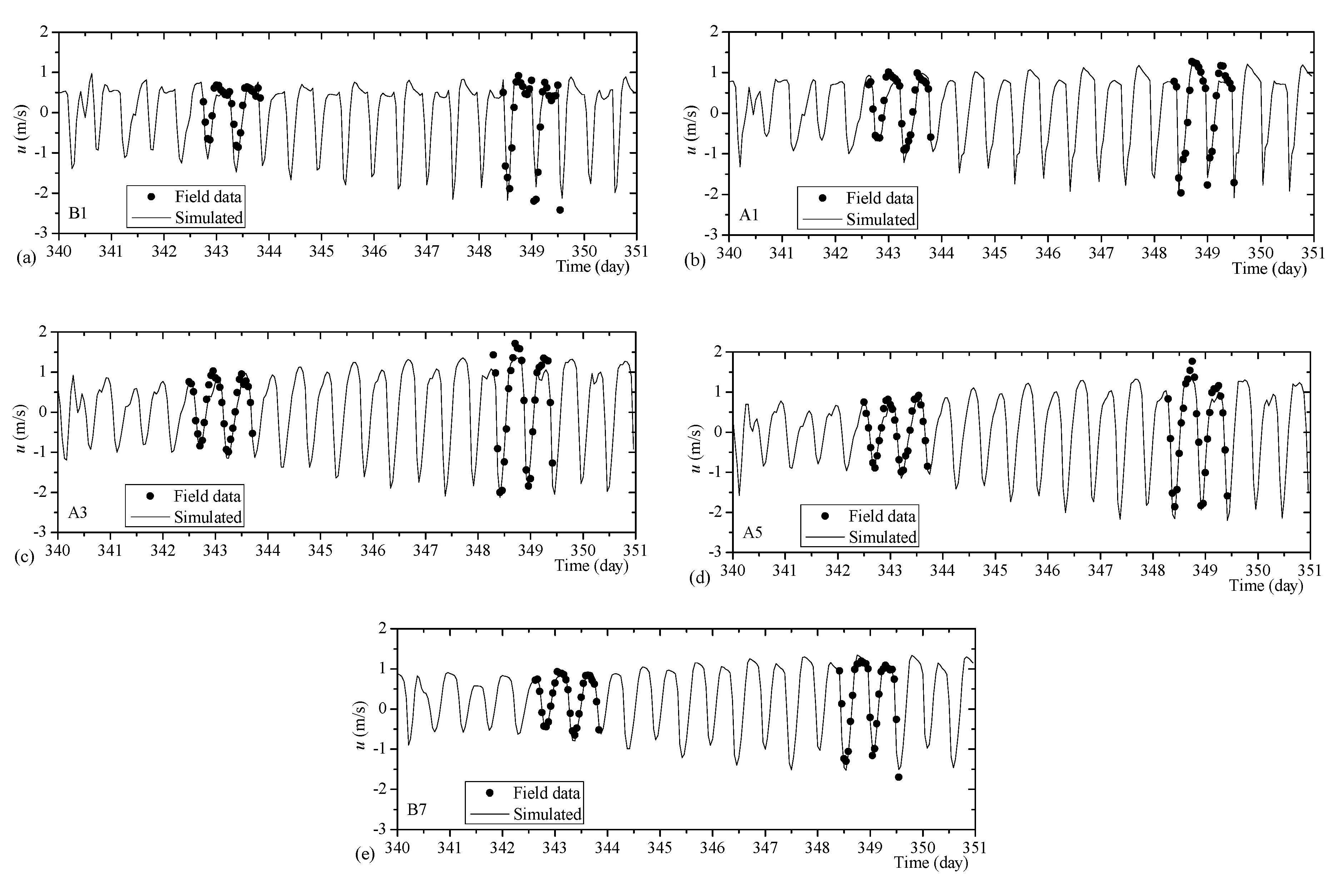
Using the aforementioned distribution of nm, the histories of the simulated tidal levels and depth-averaged velocities were shown to agree well with field data. Generally, the mean absolute error in simulated tide levels was less than 0.15 m compared with the field data, while the mean absolute relative error in simulated velocity at survey positions was less than 10%. The accuracy of the model was then verified by simulating a full spring-neap tide process on 6–16 December 2012, and the simulation results are shown in Figure 4 and Figure 5.
3. Designs of the GYS Regulation in Yangtze Estuary
To improve the morphology of the North Branch of the Yangtze Estuary and reduce the flood risk of neighboring cities, a regulation was planned by building new outlet channels for the North Branch around the GYS. The GYS is located about 7.5 km downstream of Station LXG at the outlet of the North Branch (see Figure 3). According to the topographical data of 2012, the domain, which is bounded by the −2 m contour around the GYS, was 42.4 km2. The GYS is inundated during flood tides and emerges during ebb tides. There are deep-water channels on both the south and north sides of the GYS. The riverbed elevations of the south and north deep-water channels are −12 to −13 m and −10 to −12 m, respectively. It was suggested that a series of dikes be built around the GYS to redirect and narrow the outlet channel of the North Branch.
3.1. Three Designs of Outlet Regulation
Design 1 (using two outlet channels, 11.0 km wide): A circular closed dike, which is 25.2 km long and has a top elevation of 6.0 m, is arranged along the −2 m contour of the GYS. Using the circular dike (the 0# dike), the GYS becomes an isolated island that will not be flooded during flood tides. Two channels are then formed, respectively, on the south and the north sides of the GYS to serve as the new branching outlet of the North Branch.
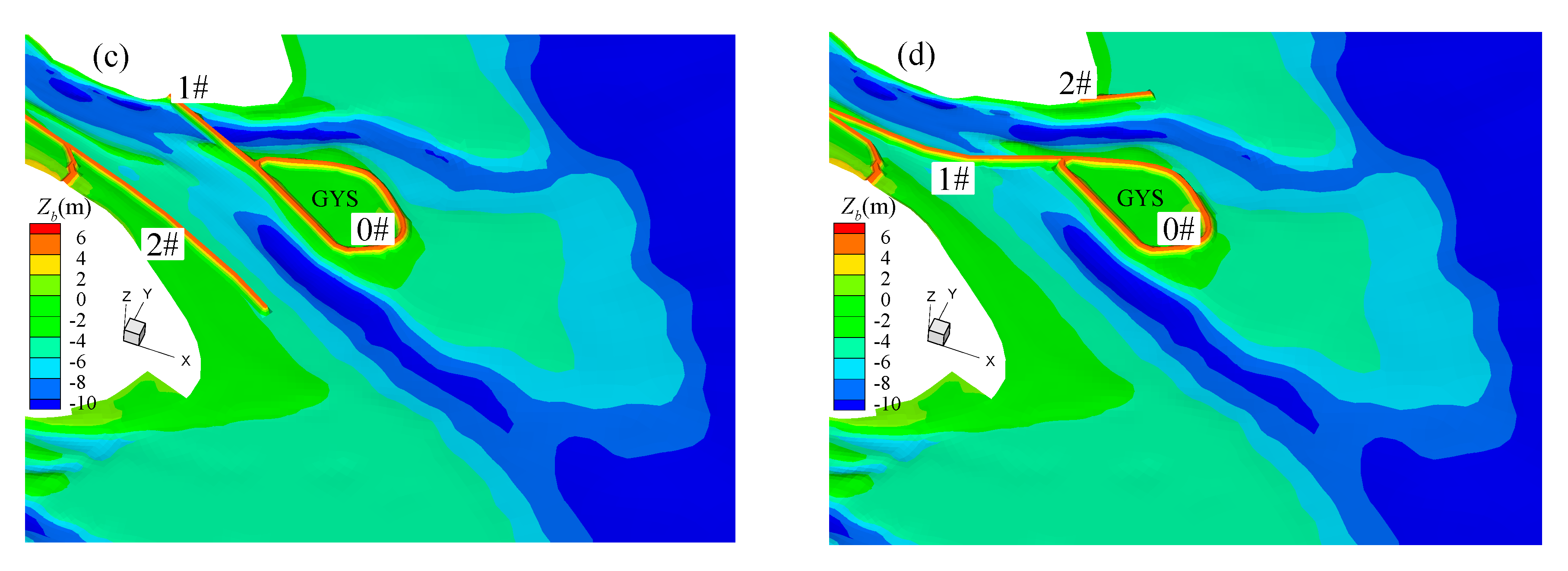
Design 2 (using a southward outlet channel, 6.5 km wide): Based on the circular dike of Design 1, the outlet of the North Branch is redirected by two new dikes and a southward outlet channel is formed. The 1# dike (7.4 km long), which connects the LXG dike and the head of the GYS, blocks the north channel of the GYS. The 2# dike (16.8 km long) starts at the north bank of the CM island and extends outside along the north edge of this island.
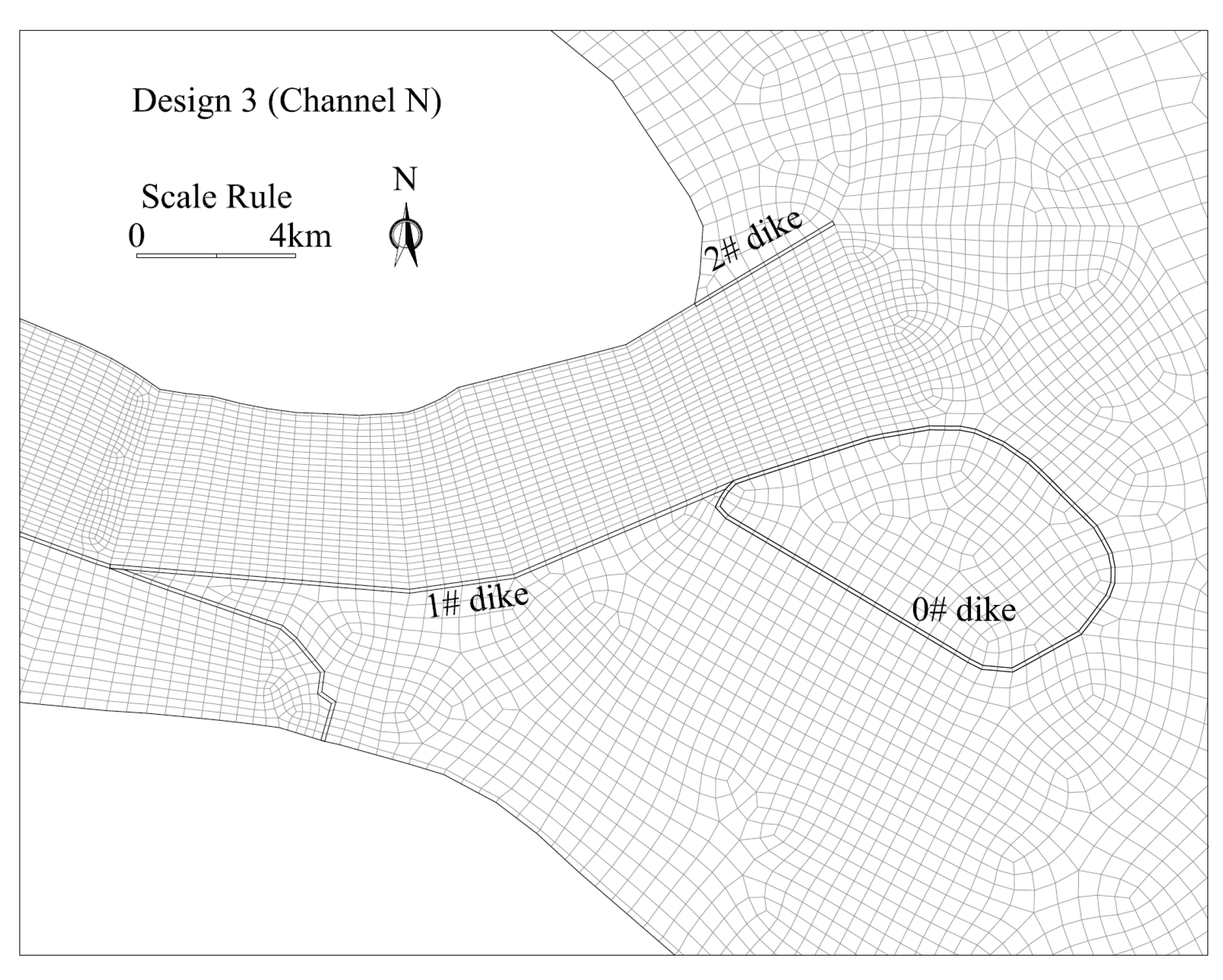
Design 3 (using a northward outlet channel, 4.5 km wide): Based on the circular dike of Design 1, the outlet of the North Branch is redirected by two new dikes and a northward outlet channel is formed. The 1# dike (16.2 km long), which connects the north bank of the CM island and the head of the GYS, blocks the south channel of the GYS. The 2# dike (6.0 km) starts at the LXG dike and extends outside along the high contour.
3.2. Description of Dikes in Model
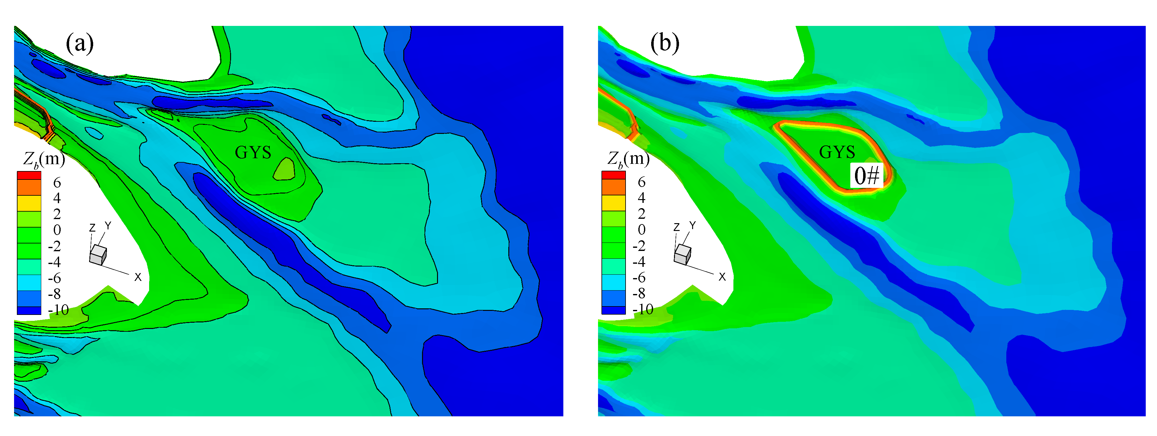
Techniques of local refinements and modifications of the unstructured grid are used to describe the dikes in different designs. First, the boundaries of dikes are sketched, according to which the local grid of the fundamental mesh is modified and refined. The resulting mesh therefore fits the dikes in the horizontal plane. The grid around the dikes of Design 3 is taken as an example, as shown in Figure 6. Second, the elevations of the grid nodes within the bound of dikes are reset according to the designed height of the dikes, to describe the entity of the constructions (see Figure 7).
It must be pointed out that: the adopted model is unconditionally stable with respect to the gravity wave speed and flow advection, by combing the θ semi-implicit method and a point-wise ELM. As a result, the local refinement of the computational grid almost does not impose any extra restrictions on the stability of the numerical model, and large time steps are still allowed.
4. Response Mechanics of Tidal Process to GYS Regulation
The property of rotational tidal flows around the outlets of the North Branch is analyzed, and the responses of the flows to the GYS regulation are studied.
4.1. Irregular Rotational Tidal Flows around GYS
Based on preliminary simulations, irregular rotational flows around the GYS can be described in five stages (the initial flow direction is southward in the following illustration).
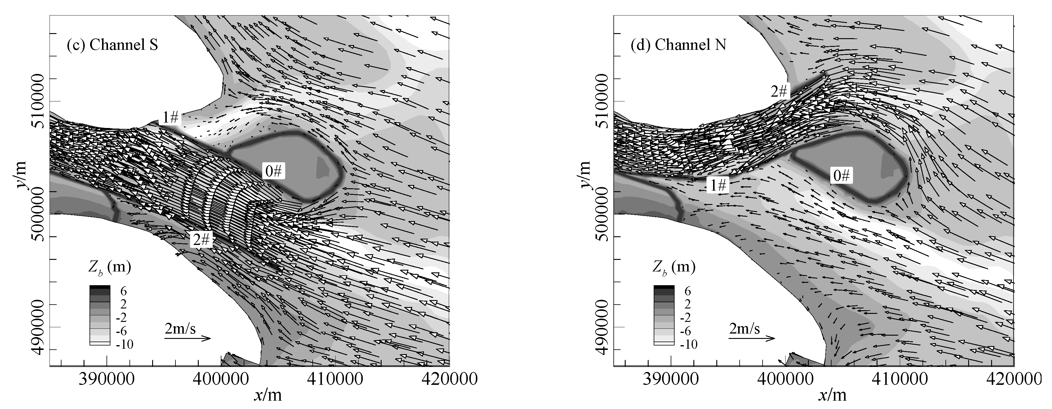
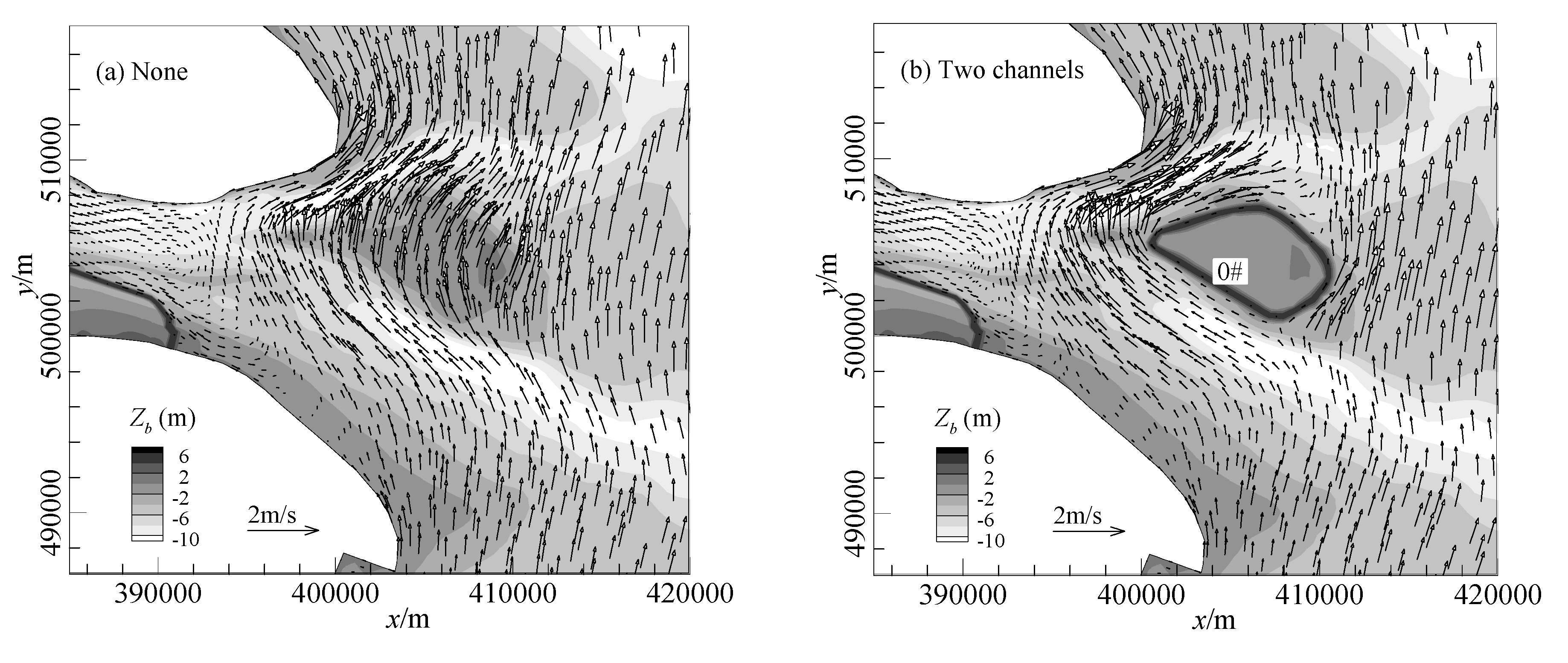
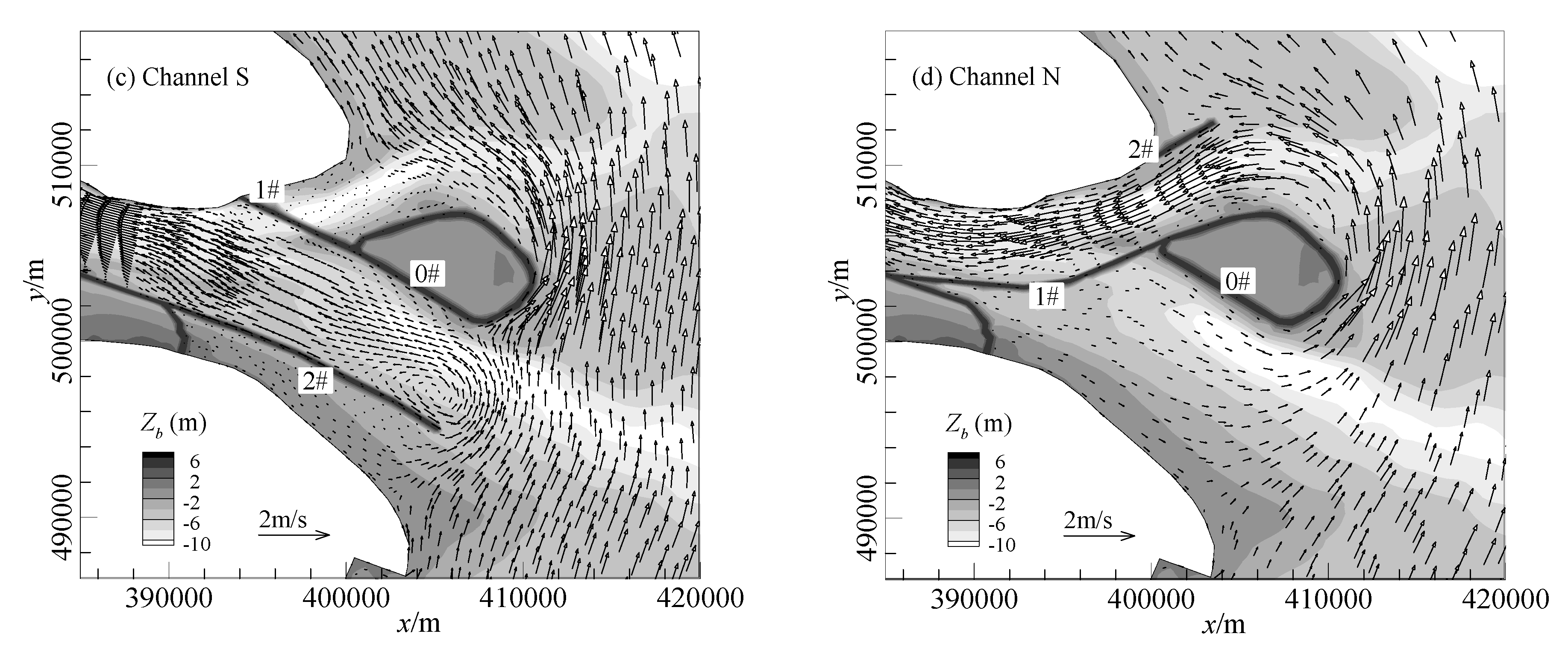
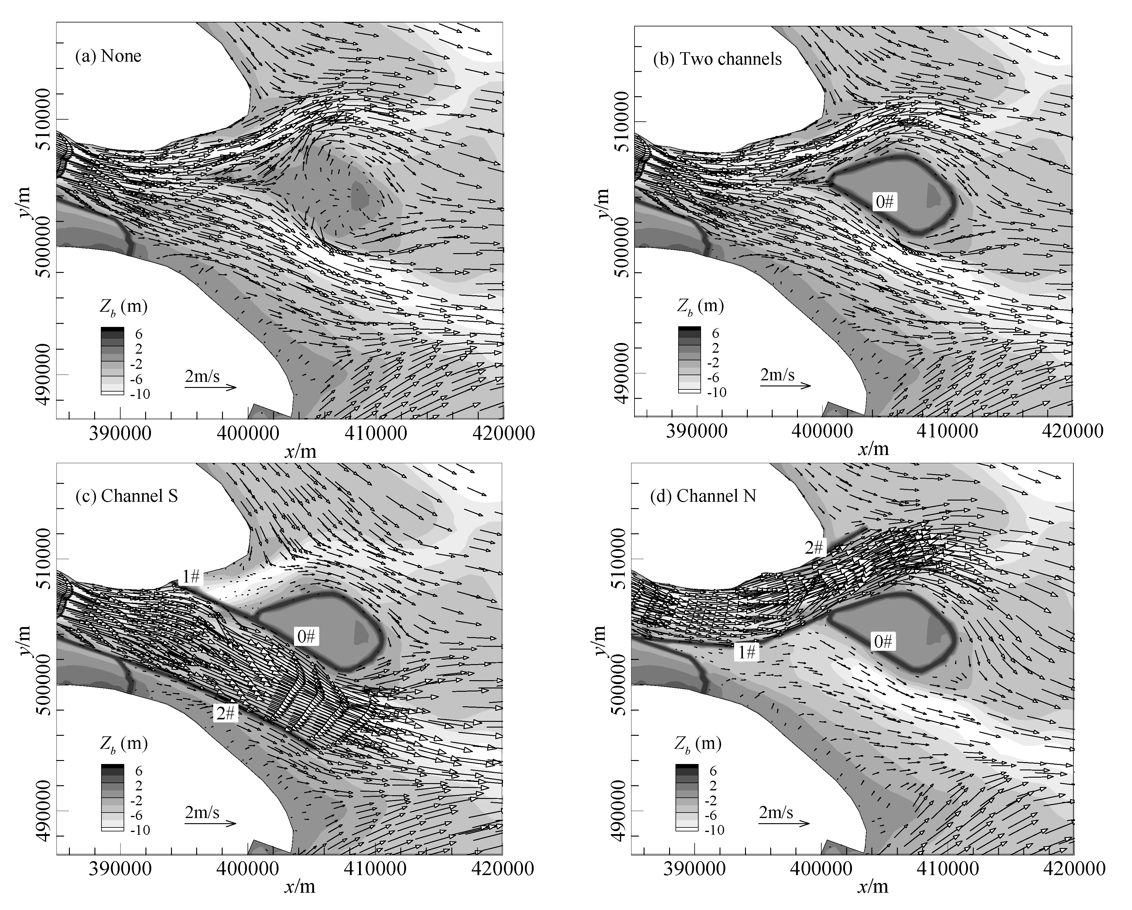
In Stage 1, ocean current turn from the south to the west in offshore regions, resulting in landward tidal flows outside the estuary. The landward flood tide reaches the North Branch earlier than the South Branch. In Stage 2, ocean currents in offshore regions continue to rotate clockwise. When it points 30° west by north, a flood-tide peak around the GYS is reached, as shown in Figure 8a. In Stage 3, the tides at the northern sea boundaries of the simulated domain are the first to ebb, relative to those at the eastern and southern sea boundaries. Northward ocean currents along the coastline are formed, when the variation of tidal flows in North Branch enters a period of transition from the flood-tide to the ebb-tide peaks. The velocity field around the GYS at a time during this period is shown in Figure 9a. In Stage 4, around the GYS, an ebb-tide peak comes about six hours after the flood-tide peak, for which the velocity field is shown in Figure 10a. In Stage 5, ocean currents outside the estuary recover to be southward after a complete rotation.
The tidal flows around the GYS are rotational and become irregular under the influences of the runoff-tide interactions, rapidly varying topographies and complex solid boundaries in coastal areas. Moreover, along the North Branch, the width of the main channel is 1 km, 1–3 km, 3–5 km, and 5–8 km, sequentially, in the upper, middle, lower and tail reaches. The upper reach of the North Branch is narrow and almost orthogonal to the South Branch. The propagation and deformation of landward irregular tidal flows in the North Branch are therefore also complex.
4.2. Effects of GYS Regulation
Through building regulation constructions (e.g., dikes) and forming new solid boundaries, the GYS regulation leads to complex disturbances to neighboring irregular rotational tidal flows, and reshapes the tidal processes of the branches in the Yangtze Estuary. Besides a common resist effect (arising from the narrowed outlet channel), a guide effect is also found when a southward outlet channel and clockwise rotational tidal flows meet. These effects are analyzed as follows.
4.2.1. Resist Effect
The conveyance capacity of a channel scales with the width of the channel, and the width of the outlet channel in the GYS regulation is defined as the sum of channel widths at the head of the GYS. This width is reduced to 11 km, 6.5 km and 4.5 km, respectively after the regulation of Design 1, 2 and 3, from the original width of 17 km. The “narrowing” retards both the flood-tide and ebb-tide flows that go through the outlet of the North Branch (defined as “resist effect”).
Under the influence of a narrowed outlet channel, the reshaped flood-tide processes along the North Branch are analyzed. During the first half of a flood-tide period, some of the landward flow from the sea lags outside the outlet. Correspondingly, flood-tide discharges at cross-sections along the North Branch are reduced. During the second half of a flood-tide period, one part of the lagging water goes landward through the outlet, while the other part is not able to go through the outlet in time and flows away to the sea. The former part of the lagging water enlarges the discharge during the second half of a flood-tide period and prolongs the duration of the flood-tide, while the latter part leads to a reduction of the landward flood-tide water flux at cross-sections. In this way, peaks of water levels and discharges at cross-sections along the North Branch during the flood-tide are both reduced and delayed, with the curves (describing the histories of them) becoming flatter.
The resist effect of the GYS regulation on ebb-tide flows is similar to that on flood-tide flows, with the peaks of water levels and discharges along the North Branch being reduced and delayed. Moreover, because the conveyance capacity of the outlet channel of the North Branch is reduced, some of its original seaward ebb-tide water flux is diverted into the South Branch.
4.2.2. Guide Effect
The dikes block or guide the irregular rotational tidal flows around the GYS and help to form new flow regimes at the outlet of the North Branch. It is interesting to find that using different designs, the disturbances of the regulation to the tidal flows around the GYS are different, which further leads to quite different influences on tidal processes along the North Branch.
As mentioned in Section 4.1, the clockwise rotational tidal flow around the GYS experiences a “transition period” between the flood-tide and ebb-tide peaks. The disturbances of the regulation to the northward tidal flows around the GYS during the transition period are different under different designs, as shown in Figure 9. For Design 3, directions of the new outlet channel and the near-shore ocean current are consistent, and the northward long dikes exert a minor influence on the northward near-shore currents around the GYS during the transition period (see Figure 9d). For Design 2, some of the northward near-shore ocean current is guided into the outlet channel of the North Branch (see Figure 9c) during the transition period, goes landward and reshapes tidal processes along the North Branch. This effect is defined as the “guide effect” whose influences are analyzed as follows.
In the second half of the flood-tide period, the guide effect of the southward dikes of Design 2 is gradually formed. The northward near-shore ocean current, which is guided into the North Branch through the southward outlet, is defined as the guided current. Because of the guided current, the flood-tide discharges, the water levels and the landward water fluxes at cross-sections along the North Branch are all enlarged relative to a case without regulations. The duration of large flood-tide discharges at these cross-sections is prolonged. Moreover, an extra storage of water is formed along the North Branch, which is defined as the guided storage. The discharge of the guided current is reduced with respect to the distance of its landward travel. Correspondingly, the guided storage in the upper reach of the North Branch is smaller than that in the lower reach.
During the ebb-tide period, the guided storage moves seaward along with ebb-tide flows and increases the ebb-tide discharge at cross-sections along the North Branch. A larger guided storage in the lower reach causes a larger increment of discharge at cross-sections of the lower North Branch.
4.2.3. Overlapped Effects of GYS Regulation
The guide effect, together with common the resist effect, reshapes the estuarine tidal processes of the Yangtze Estuary. Responses of tidal variables (discharges, water levels, and water fluxes) at cross-sections along the North Branch to the regulation are listed in Table 2, where the guide effect columns are especially for Design 2 with a southward outlet channel. The duration of a flood/ebb-tide is divided into two parts (first half and second half) approximately according to the time of peak discharges at the outlet of the North Branch. The resist effect (Resist-E.) plays a role all through the flood and ebb tides. The guide effect exists only in the case of Design 2, and mainly plays a role in the second half of the flood-tide period and the first half of the ebb-tide period.
The resist effect and the guide effect may enhance each other but at other times counteract each other, in reshaping the process of tidal variables at cross-sections of the North Branch. When the two effects counteract each other, it is often difficult to determine the overlapped result. Moreover, the details of a design and the environment factors both contribute to increasing the uncertainty of the overlapped result of the resist effect and the guide effect at different locations of the North Branch. The details of a design are mainly the width of the outlet channel, the direction of the outlet and so on. Environmental factors include the trumpet-shaped morphology of the North Branch and the irregularity of rotational tidal flows around the GYS. As a result, the responses of tidal variables at cross-sections along the North Branch to the GYS regulation are complex.
4.3. Responses of Flow Regime to Different Designs
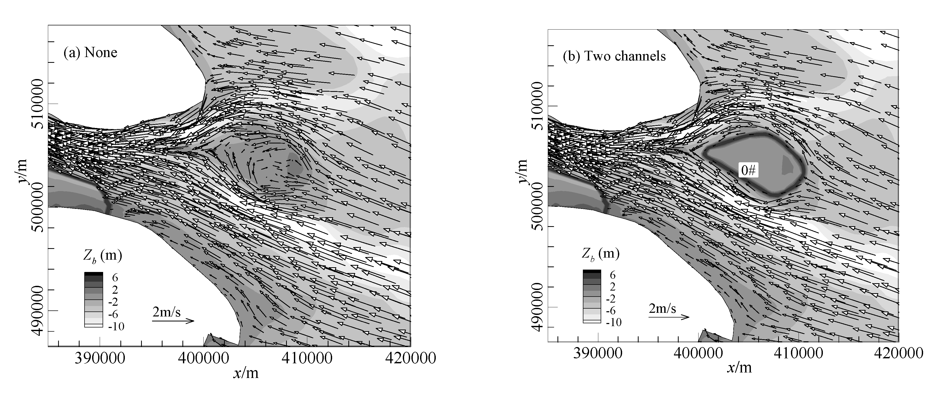
At the flood-tide peak (t = 12 h), the simulated velocity fields around the GYS under different designs are shown in Figure 8b–d. The simulated velocity field under Design 1 is similar to that with no regulation. The circular dike around the GYS causes minor disturbances to neighboring tidal flows, because only the high-elevation region of the GYS is isolated from the flow conveyance area. Using Designs 2 and 3, the landward flood-tide flow is confined to the south and north channels beside the GYS, respectively. The width of the outlet channel of Design 3 (4.5 km) is smaller than that of Design 2 (6.5 km), so Design 3 may produce a stronger resist effect than Design 2. Moreover, the flood-tide flow has a longer and more curving path under Design 3 than Design 2. It is therefore more difficult for the landward flood-tide flow to go through the outlet under Design 3.
At a time of flood-ebb transition (t = 15 h), the simulated velocity fields around the GYS under different designs are shown in Figure 9b–d. Under Design 1, northward near-shore flow is divided into two parts which bypass the GYS, respectively, and continues to go northward. Using Designs 2 and 3, some lagged water outside the outlet (by the resist effect during the first half of a flood-tide period) goes landward through the outlet. Relative to Design 3, Design 2 blocks the north channel of the GYS, namely the outgoing way of the tidal current entering the south channel of the GYS. The southward outlet of Design 2 helps guide the northward near-shore ocean current into the North Branch of the Yangtze Estuary (the guide effect).
At the ebb-tide peak (t = 18 h), the simulated velocity fields around the GYS under different designs are shown in Figure 10b–d. Under different designs, the resist effect of the narrowed outlet channel on tidal flows during flood tides is similar to that during ebb tides. Because an ebb-tide process is longer and flatter than a flood-tide process, the influence of the GYS regulation on the ebb-tide process is relatively mild.
5. Quantitative Study on Influences of GYS Regulation
The three designs of the GYS regulation were studied using a condition of dry-season runoff and spring tide, when the regulation is regarded to cause more significant influence on tidal flows. At the upstream boundary, the river discharge was set to 19,000 m3/s, and the inflow water flux was calculated to be 16.41 × 10⁸ m3 per day. The seaward boundaries are forced by water-level histories of periodic spring tides. The simulations were run using Designs 1–3 (denoted as T Ch., Ch. S and Ch. N, respectively). In total, four simulations were run, and the results of the simulations with different designs were compared with those without a regulation.
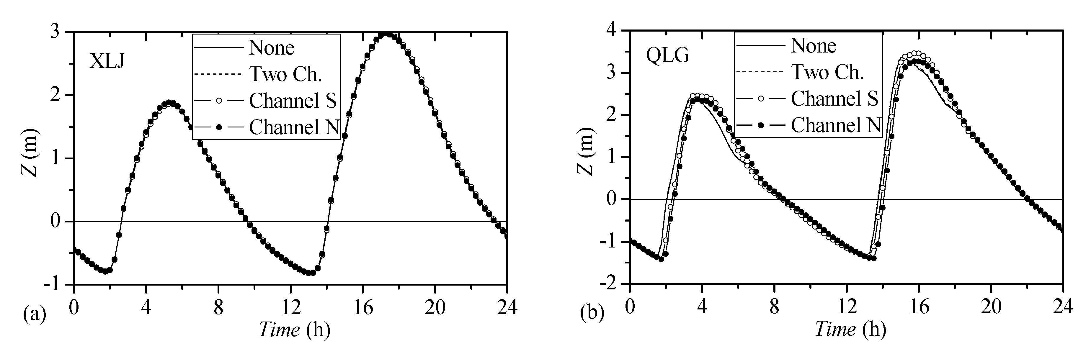
The GYS regulation reshapes estuarine tidal process, resulting in new histories of discharges (Q) and water levels (Z) at cross-sections of the tidal reaches. Histories of the simulated Q and Z were recorded at seven cross-sections and 14 gauges (see Figure 3), respectively. For each cross section, the histories of Q could be integrated over the flood-tide and the ebb-tide periods, respectively, to obtain the cross-sectional water fluxes (CSWFs) of the corresponding period. The histories of the simulated Q and Z at cross-sections are plotted in Figure 10 (variation in 24 h).
According to the simulation results, the influence of the GYS regulation on tidal processes of cross-sections is mainly confined to the domain downstream of XLJ. The regulation reshapes the tidal processes at cross-sections of the North Branch directly, and only leads to a secondary influence on tidal flows of the South Branch. Under a given design, the changes in Q, CSWF and Z of the North Branch will be much larger than those of the South Branch. Moreover, under a given design, the overlapped results of the resist effect and the guide effect vary at different locations along the North Branch and at different times, resulting in different deformations of tidal processes.
5.1. Responses of Discharge to GYS Regulation
The simulated histories of the Q with the GYS regulation were compared with those with no regulation, as shown in Figure 11. Variations of discharge processes under different regulations are here represented quantitatively by the changes in discharge peak (Qpeak) and CSWF at cross-sections, which are listed, respectively, in Table 3 and Table 4.
5.1.1. Variation of Flood-Tide Q along North Branch
Under Design 1, the weak resist effect caused by the circular closed dike only leads to minor reductions in Qpeak and CSWF at cross-sections along the North Branch. Under Design 3, only the resist effect exists, and reductions of Qpeak and CSWF are significant. The histories of the flood-tide discharge at cross-sections along the North Branch shrink sharply.
Under Design 2, on the one hand, the resist effect reduces the Qpeak and CSWF at cross-sections. On the other hand, the landward guided current increases the flood-tide discharge at cross-sections, and the increment decreases from the lower to the upper North Branch. The overlapped results of the resist effect and the guided current vary along the North Branch. In middle and lower reaches, the resist effect plays a main role and leads to a reduction of Qpeak at Stations Sanhegang (SHG) and Santiaogang (STG). Despite the reduction of the Qpeak, the CSWFs at Station SHG and STG are still increased because of an enlarged duration of large flood-tide discharges. In the upper reaches, the guided current deforms during its landward travel, whose result accounts for the increase of Qpeak at Station QLG (see Figure 11). The CSWF at Station QLG is reduced because the effect of the weakened guided current is not strong enough to counteract the influence of the resist effect there.
5.1.2. Variation of Ebb-Tide Q along North Branch
Under Design 1, the weak resist effect caused by the circular closed dike only leads to minor reductions in Qpeak and CSWF at cross-sections along the North Branch. Under Design 3, only the resist effect exists, and reductions of Qpeak and CSWF are significant. The histories of the flood-tide discharge at cross-sections along the North Branch shrink sharply.
Under Design 2, on the one hand, the resist effect reduces Qpeak and CSWF at cross-sections. On the other hand, the guided storage (formed by the guided current during the flood-tide period) transforms into seaward flows, which moves along with ebb-tide flows, leading to an increment of the cross-sectional ebb-tide discharge. Consistent with the distribution of the guided storage along the North Branch, the increment of ebb-tide discharge is smaller in upper reaches and larger in lower reaches. The overlapped results of the resist effect and the guided storage vary along the North Branch. At the lower reaches, the increment of the ebb-tide discharge caused by the guided storage exceeds the decrement caused by the resist effect, leading to an increase of the ebb-tide Qpeak and CSWF at Station STG. At the upper and middle reaches, a smaller guided storage is not strong enough to counteract the resist effect, leading to a reduction of the ebb-tide Qpeak and CSWF.
5.2. Responses of Water Level to GYS Regulation
The simulated histories of the Z with the GYS regulation were compared with those with no regulation in Figure 11. Variations of water-level processes under different regulations are here represented quantitatively by the changes in water-level peaks (Zpeak) at cross-sections (listed in Table 5), which is often considered as an important indicator for regional flood defense.
The influence of the GYS regulation on water-level processes was revealed to be mainly confined to the North Branch. Under a given design, the changes in Zpeak at cross-sections were determined by the overlapped results of the resist effect and the guide effect, which vary along the North Branch. Moreover, the changes in Zpeak at cross-sections along the North Branch are found to be closely related to the changes in Qpeak and CSWF, and are analyzed as follows.
Under Design 1, the weak resist effect of the regulation leads to only minor variations in Zpeak at cross-sections along the North Branch. Under Design 3, only the resist effect exists, and the Zpeak is significantly reduced at cross-sections during a flood-tide. The histories of the flood-tide water levels at cross-sections along the North Branch shrink sharply.
Under Design 2, on the one hand, the resist effect reduces Zpeak at cross-sections by limiting the flood-tide discharge. On the other hand, the landward guided current pushes up the Zpeak by increasing flood-tide discharges at cross-sections. In the lower and middle reaches, water levels at cross-sections are increased by the accumulative effect of the strong guided current, leading to a significant increase of 21.7–23.4 cm in Zpeak at Station SHG and STG. The water level of the upper reach is uplifted by the downstream high water level, so the Zpeak at Station QLG is also increased.
6. Discussion
6.1. Specialty of the Studied Problem
According to the location of the regulation projects in an estuary, these projects may be divided into inner, outlet and offshore regulations as follows.
An inner regulation, such as reclamations and reservoirs [4,6], is located in tidal reaches inside an estuary. The inner regulation interacts with bidirectional tidal flows, and its influence is mainly confined to the tidal reaches inside the estuary. An offshore regulation, such as harbors around an island [12,27], is located in offshore domains outside of an estuary. The offshore regulation interacts with rotational tidal flows of the sea, and its influence is mainly confined to the neighboring sea.
An outlet regulation [28,29] is located around the outlets of an estuary, which is the transition region between the bidirectional flows inside the estuary and the rotational tidal flows in offshore regions. First, the disturbances of an outlet regulation to tidal flows vary with respect to the periodical variation of irregular rotational tidal flows. Second, the influence of an outlet regulation on tidal flows will cover a widespread domain, reaching both tidal reaches inside the estuary and offshore domains outside. Third, in branching estuaries such as the Yangtze Estuary, the outlet regulation will change the exchange of water between different branches of the estuary.
As an outlet regulation in a three-level branching estuary, influences of the GYS regulation on estuarine tidal flows are much more complex than those of inner and offshore projects. To our best knowledge, studies on the response mechanics of irregular rotational tidal flows to outlet regulation in complex branching estuaries have not been reported yet.
6.2. The Most Important Findings
Three designs of the GYS regulation were studied, including various diversion dikes and new outlets of different widths. The most important finding of this study is that: additional current and additional storage are formed along the North Branch when a southward outlet and the clockwise rotational flow met around GYS. This interesting phenomenon is named “guide effect” in this study. The guide effect, together with common resist effect, reshapes the estuarine tidal processes.
On the one hand, based on the guide effect theory, response mechanics of irregular rotational tidal flows to the outlet regulation in complex branching estuaries are clarified.
On the other hand, design issues, which are different with our former experience of arranging the constructions, are suitably explained. Design 2 (outlet channel is 6.5 km wide) requires milder shrinkage of the current outlet than Design 3 (outlet channel is 4.5 km wide). Moreover, the southward outlet channel of Design 2 has the same direction as that of the tail reach of the North Branch and is more fluent. Before this study, the original choice is Design 2 which was expected to lead to milder disturbances to estuarine tidal flows. However, the study finds that: the peaks of water levels along the North Branch are increased by 21.7–23.4 cm under Design 2, because of the guide effect. Such a significant increase of the water-level peaks is not acceptable in terms of flood defense. As a result, Design 3, which could reduce the water-level peaks, is recommended instead of Design 2. The new knowledge also provides references for other real estuarine projects.
7. Conclusions
Responses of irregular rotational tidal flows to an outlet regulation (the GYS regulation) in the three-level branching Yangtze Estuary are studied by numerical simulations and theoretical analysis. A two-dimensional (2D) numerical model was developed to study the hydrodynamic issues of the GYS regulation. A high-resolution channel-refined unstructured grid (about 200,000 cells) was used, which ensured a good description of the river–coast–ocean coupling, the irregular boundaries and the local river regimes in the Yangtze Estuary. The model was in tests revealed to be accurate enough to be used to study the tidal flows and related problems in the estuary.
Three designs of the GYS regulation are presented, which are Design 1 (using two outlet channels), Design 2 (using a southward outlet channel), and Design 3 (using a northward outlet channel). It was interesting to find that additional current and additional storage are formed along the North Branch when a southward outlet and the clockwise rotational flow met around GYS. This phenomenon is named “guide effect” in this study. The guide effect, together with common resist effect, reshapes the estuarine tidal processes. Based on the guide effect theory, response mechanics of irregular rotational tidal flows to the outlet regulation in branching estuaries are clarified.
Using the guide effect theory, the three regulation designs of the GYS regulation are evaluated. Design 2 (with southward dikes) is found to suffer from significant guided current and storage, increasing the peak of water levels along the North Branch and the threat of flood. Design 3, which is free of the guide effect and reduces water-level peaks, is finally recommended.
Supplementary Materials
The following are available online at https://www.mdpi.com/2073-4441/11/7/1445/s1, Figure S1: Channel-refined computational grid for numerical model of Yangtze Estuary.
Author Contributions
Conceptualization, D.H., M.W., and S.Y.; methodology, D.H., and M.W.; software, D.H.; validation, D.H., M.W., and S.Y.; formal analysis, D.H. and M.W.; investigation, D.H.; resources, S.Y. and Z.J.; data curation, M.W., S.Y. and Z.J.; writing—Original draft preparation, D.H., and M.W.; writing—Review and editing, Z.J.; visualization, Z.J.; supervision, M.W. and S.Y.; project administration, S.Y.; funding acquisition, M.W. and Z.J.
Funding
Financial support from Science and Technology Program of Guizhou Province, China (Grant No. 2017-3005-4), the Fundamental Research Funds for the Central Universities (2017KFYXJJ197), China’s National Natural Science Foundation (51339001, 51779015 and 51479009) are acknowledged.
Conflicts of Interest
The authors declare no conflict of interest.
Notation
The following symbols and abbreviations are used in this paper:
| 2D | two-dimensional |
| Ch. S | Southward Channel (Design 2) |
| Ch. N | Northward Channel (Design 3) |
| CSWF | cross-sectional water flux |
| CM | Chong-Ming Island; |
| ELM | Eulerian–Lagrangian method; |
| f | Coriolis factor; |
| g | gravitational acceleration; |
| GYS | Gu-Yuan Sand; |
| GTM | Global Tide Model; |
| h(x, y, t) | water depth; |
| LXG | Station Lian-Xin-Gang; |
| nm | Manning’s roughness coefficient; |
| QLG | Station Qing-Long-Gang; |
| STG | Station San-Tiao-Gang; |
| SWEs | shallow water equations; |
| t | time; |
| T Ch. | Two channels (Design 1); |
| u(x, y, t) | x-direction component of vertically averaged velocity; |
| v(x, y, t) | y-direction component of vertically averaged velocity; |
| υt | coefficient of the horizontal eddy viscosity; |
| XLJ | Station Xu-Liu-Jing; |
| η(x, y, t) | water level measured from an undisturbed reference water surface; |
| ρ | the water density; |
| τsx | wind stress in the x-directions; |
| τsy | wind stress in the y-directions; |
| Ω | angular velocity of rotation of the Earth; |
| φ | latitude of the reference location. |
References
- Wu, H.; Zhu, J.R.; Chen, B.R.; Chen, Y.Z. Quantitative relationship of runoff and tide to saltwater spilling over from the North Branch in the Changjiang Estuary, A numerical study. Estuar. Coast. Shelf Sci. 2006, 69, 125–132. [Google Scholar] [CrossRef]
- Li, T.L.; Li, Y.C.; Gao, X.Y.; Wang, Y.G. Effects of regulation project on salinity intrusion in Yangtze Estuary. Ocean Eng. 2005, 23, 31–38. (In Chinese) [Google Scholar] [CrossRef]
- Yan, Y.X.; Liu, H.W.; Wu, D.A.; Tong, C.F. Analysis of tidal characteristics before and after construction of regulation projects in Yangtze River estuary. J. Hohai Univ. (Nat. Sci.) 2009, 37, 100–104. (In Chinese) [Google Scholar] [CrossRef]
- Song, D.H.; Wang, X.H. Suspended sediment transport in the Deepwater Navigation Channel, Yangtze River Estuary, China, in the dry season 2009: 2. Numerical simulations. J. Geophys. Res. (Ocean) 2013, 118, 5568–5590. [Google Scholar] [CrossRef]
- Li, W.Z. Analysis of impacts of Ruifengsha regulation works in south channel of Yangtze River estuary on surrounding river regime. Hydro-Sci. Eng. 2014, 4, 87–90. (In Chinese) [Google Scholar] [CrossRef]
- Guo, Q.C.; Zhu, J.R. Impact of Qingcaosha reservoir project on the bed erosion and deposition nearby the water area. J. Mar. Sci. 2015, 3, 34–41. (In Chinese) [Google Scholar] [CrossRef]
- Zhou, J.F.; Li, J.C. Influences of the fish-mouth project and the groins on the flow and sediment ratio of the Yangtze River waterway. Appl. Math. Mech.-Engl. Ed. 2004, 25, 158–167. [Google Scholar]
- Wang, Y.; Shen, J.; He, Q. A numerical model study of the transport timescale and change of estuarine circulation due to waterway constructions in the Changjiang Estuary, China. J. Mar. Syst. 2010, 82, 154–170. [Google Scholar] [CrossRef]
- Ge, J.Z.; Chen, C.S.; Qi, J.H.; Ding, P.X.; Beardsley, R.C. A dike–groyne algorithm in a terrain-following coordinate ocean model (FVCOM): Development, validation and application. Ocean Model. 2012, 47, 26–40. [Google Scholar] [CrossRef]
- Ma, G.F.; Shi, F.Y.; Liu, S.G.; Qi, D.M. Migration of sediment deposition due to the construction of large-scale structures in Changjiang Estuary. Appl. Ocean Res. 2013, 43, 148–156. [Google Scholar] [CrossRef]
- Kuang, C.P.; Chen, W.; Gu, J.; He, L.L. Comprehensive analysis on the sediment siltation in the upper reach of the deepwater navigation channel in the Yangtze Estuary. J. Hydrodyn. 2014, 26, 299–308. [Google Scholar] [CrossRef]
- Zuo, S.H.; Zhang, N.C.; Li, B.; Zhang, Z.; Zhu, Z.X. Numerical simulation of tidal current and erosion and sedimentation in the Yangshan deep-water harbor of Shanghai. Int. J. Sediment Res. 2009, 24, 287–298. [Google Scholar] [CrossRef]
- Kuang, C.P.; Liu, X.; Gu, J.; Guo, Y.K.; Huang, S.C.; Liu, S.G.; Yu, W.W.; Huang, J.; Sun, B. Numerical prediction of medium-term tidal flat evolution in the Yangtze Estuary, impacts of the Three Gorges project. Cont. Shelf Res. 2013, 52, 12–26. [Google Scholar] [CrossRef]
- Hu, D.C.; Zhong, D.Y.; Zhang, H.W.; Wang, G.Q. Prediction–Correction Method for Parallelizing Implicit 2D Hydrodynamic Models I Scheme. J. Hydraul. Eng. 2015, 141, 04015014. [Google Scholar] [CrossRef]
- Hu, D.C.; Zhong, D.Y.; Zhu, Y.H.; Wang, G.Q. Prediction–Correction Method for Parallelizing Implicit 2D Hydrodynamic Models II Application. J. Hydraul. Eng. 2015, 141, 06015008. [Google Scholar] [CrossRef]
- Hu, D.C.; Zhu, Y.H.; Zhong, D.Y.; Qin, H. Two-Dimensional Finite-Volume Eulerian-Lagrangian Method on Unstructured Grid for Solving Advective Transport of Passive Scalars in Free-Surface Flows. J. Hydraul. Eng. 2017, 143, 04017051. [Google Scholar] [CrossRef]
- Hu, D.C.; Yao, S.M.; Qu, G.; Zhong, D.Y. Flux-form Eulerian-Lagrangian Method for Solving Advective Transport of Scalars in Free-Surface Flows. J. Hydraul. Eng. 2019, 145. [Google Scholar] [CrossRef]
- Casulli, V.; Zanolli, P. Semi-implicit numerical modeling of nonhydrostatic free-surface flows for environmental problems. Math. Comput. Model. 2002, 36, 1131–1149. [Google Scholar] [CrossRef]
- Dimou, K. 3-D Hybrid Eulerian–Lagrangian/Particle Tracking Model for Simulating Mass Transport in Coastal Water Bodies. Ph.D. Thesis, Department of Civil Engineering, Massachusetts Institute of Technology, Cambridge, MA, USA, 1992. [Google Scholar]
- Zhang, Y.L.; Baptista, A.M.; Myers, E.P. A cross-scale model for 3D baroclinic circulation in estuary-plume-shelf systems, I. Formulation and skill assessment. Cont. Shelf Res. 2004, 24, 2187–2214. [Google Scholar] [CrossRef]
- Cheng, Y.C.; Andersen, O.B.; Knudsen, P. Integrating Non-Tidal Sea Level data from altimetry and tide gauges for coastal sea level prediction. Adv. Space Res. 2012, 50, 1099–1106. [Google Scholar] [CrossRef]
- Wu, S.H.; Cheng, H.Q.; Xu, Y.J.; Li, J.F.; Zheng, S.W.; Xu, W. Riverbed Micromorphology of the Yangtze River Estuary, China. Water 2016, 8, 190. [Google Scholar] [CrossRef]
- Chen, C.S.; Xue, P.F.; Ding, P.X.; Beardsley, R.C.; Xu, Q.C.; Mao, X.M.; Gao, G.P.; Qi, J.H.; Li, C.Y.; Lin, H.C.; et al. Physical mechanisms for the offshore detachment of the Changjiang Diluted Water in the East China Sea. J. Geophys. Res. 2008, 113, C02002. [Google Scholar] [CrossRef]
- Xue, P.F.; Chen, C.S.; Ding, P.X.; Beardsley, R.C.; Lin, H.C.; Ge, J.Z.; Kong, Y.Z. Saltwater intrusion into the Changjiang River, A model-guided mechanism study. J. Geophys. Res. 2009, 114, C02006. [Google Scholar] [CrossRef]
- Cao, Z.Y. A Two-Dimensional Non-Uniform Sediment Numerical Model for the Yangtze Estuary. Ph.D. Thesis, East China Normal University, Shanghai, China, 2003. (In Chinese). [Google Scholar]
- Shi, Y.B.; Lu, H.Y.; Yang, Y.P.; Cao, Y. Prediction of erosion depth under the action of the exceptional flood in the river reach of a tunnel across the Qiantang estuary. Adv. Water Sci. 2008, 19, 685–692. (In Chinese) [Google Scholar] [CrossRef]
- Ying, X.; Ding, P.; Wang, Z.B.; Van Maren, D.S. Morphological impact of the construction of an offshore Yangshan Deepwater Harbor in the Port of Shanghai, China. J. Coast. Res. 2012, 28, 163–173. [Google Scholar] [CrossRef]
- Xie, R.; Wu, D.A.; Yan, Y.X. Fine silt particle pathline of dredging sediment in the Yangtze River deepwater navigation channel based on EFDC model. J. Hydrodyn. 2010, 22, 760–772. [Google Scholar] [CrossRef]
- Pan, L.; Ding, P.; Ge, J. Impacts of Deep Waterway Project on morphological changes within the North Passage of the Changjiang Estuary, China. J. Coast. Res. 2012, 28, 1165–1176. [Google Scholar] [CrossRef]
Figure 1.
The location of the Yangtze Estuary and the study area (a Google Map that shows the geographical features of the location).
Figure 1.
The location of the Yangtze Estuary and the study area (a Google Map that shows the geographical features of the location).

Figure 2.
Description of the bound, the three-level bifurcations and the strong river-coast-sea coupling in Yangtze Estuary (computational domain and grid are also given).
Figure 2.
Description of the bound, the three-level bifurcations and the strong river-coast-sea coupling in Yangtze Estuary (computational domain and grid are also given).

Figure 3.
Arrangements of hydrology survey locations in Yangtze Estuary.

Figure 4.
Comparisons of the simulated tide-level histories and field data. (a) at Station Xuliujing (XLJ), (b) at Station Qinglonggang (QLG), (c) at Station Lianxingang (LZG), (d) at Station Nanmen (NM), (e) at Station Hengsha (HS).
Figure 4.
Comparisons of the simulated tide-level histories and field data. (a) at Station Xuliujing (XLJ), (b) at Station Qinglonggang (QLG), (c) at Station Lianxingang (LZG), (d) at Station Nanmen (NM), (e) at Station Hengsha (HS).


Figure 5.
Comparisons of simulated histories of velocity with field data (negative velocity is landward velocity, which appears during the flood duration). (a) at Survey Point B1, (b) at Survey Point A1, (c) at Survey Point A3, (d) at Survey Point A5, (e) at Survey Point B7.
Figure 5.
Comparisons of simulated histories of velocity with field data (negative velocity is landward velocity, which appears during the flood duration). (a) at Survey Point B1, (b) at Survey Point A1, (c) at Survey Point A3, (d) at Survey Point A5, (e) at Survey Point B7.

Figure 6.
Grid refinement around dikes of the outlet regulation.

Figure 7.
Arrangements of dikes: (a) Design “None”; (b) Design 1 (using two outlet channels); (c) Design 2 (using a southward outlet channel); (d) Design 3 (using a northward outlet channel).
Figure 7.
Arrangements of dikes: (a) Design “None”; (b) Design 1 (using two outlet channels); (c) Design 2 (using a southward outlet channel); (d) Design 3 (using a northward outlet channel).


Figure 8.
Velocity fields under different designs at flood-tide (t = 12 h).


Figure 9.
Velocity fields under different designs at a time during flood-ebb transition (t = 15 h).


Figure 10.
Velocity fields under different designs at ebb-tide (t = 18 h).

Figure 11.
Histories of simulated water levels (Z) and discharges (Q) at cross-sections in the Yangtze Estuary: (a–e) Z processes; (f–j) Q processes.
Figure 11.
Histories of simulated water levels (Z) and discharges (Q) at cross-sections in the Yangtze Estuary: (a–e) Z processes; (f–j) Q processes.


Table 1.
Grid scales of high-resolution unstructured grids in Yangtze Estuary.
| Region | Length (km) | Area (km2) | Resolution of Bathymetry Graph | Grid Scale (m × m) |
|---|---|---|---|---|
| Tidal reach | 533 | 2066 | 1/10,000 | 200 × 80 |
| North branch | 80 | 366 | 1/10,000 | 200 × 80~400 × 200 |
| South branch | 88 | 1132 | 1/25,000 | 400 × 200 |
| Coast region | — | 8746 | — | 500~2000 |
| East Sea | — | 105,993 | — | 2000~5000 |
Table 2.
Responses of tidal variables at cross-sections along the North Branch to the GYS regulation.
Table 2.
Responses of tidal variables at cross-sections along the North Branch to the GYS regulation.
| Time | Flood-Tide Process | Ebb-Tide Process | ||||
|---|---|---|---|---|---|---|
| Variable | Resist-E. | Guide-E. | Variable | Resist-E. | Guide-E. | |
| First half period | Q (−) | ↓ | – | Q (+) | ↓ | ↑ |
| Z | ↓ | – | Z | ↑ | ↑ | |
| Landward FW | ↓ | – | Seaward FW | ↓ | ↑ | |
| Second half period | Q (−) | ↑ | ↑ | Q (+) | ↑ | – |
| Z | ↓ | ↑ | Z | ↑ | – | |
| Landward FW | – | ↑ | Seaward FW | – | – | |
| Total period | Q (−) peak | ↓ | ↑ | Q (+) peak | – | ↑ |
| Z (peak) | ↓ | ↑ | Z (trough) | – | – | |
| Landward FW | ↓ | ↑ | Seaward FW | ↓ | ↑ | |
Q (−) and Q (+) are the landward and the seaward discharges, respectively; Z and FW are water-level and water flux at cross-sections, respectively; “↑” means “increase” and “↓” means “decrease”; resist effect and guide effect are, respectively, denoted by “Resist-E.” and “Guide-E.”; “–” means that it is difficult to determine the variation of a variable by qualitative analysis.
Table 3.
Variations of cross-sectional discharge peaks (Qpeak) in the estuary after GYS Regulation.
| Region | Cross Section | Qpeak1 (Flood) | Flood-Tide Process (%) | Qpeak2 (Ebb) | Ebb-Tide Process (%) | ||||
|---|---|---|---|---|---|---|---|---|---|
| T. Ch. | Ch. S. | Ch. N | T. Ch. | Ch. S | Ch. N | ||||
| River | XLJ | 15.33 | −0.11 | −0.19 | −0.26 | 9.94 | −0.12 | −0.22 | −0.32 |
| North Branch | QLG | 1.44 | −0.22 | 11.72 | −23.18 | 0.67 | −3.88 | −15.05 | −26.37 |
| SHG | 3.39 | −1.21 | −4.22 | −18.35 | 1.50 | −0.65 | −11.35 | −14.48 | |
| STG | 6.24 | −1.60 | −6.87 | −18.64 | 3.07 | −0.11 | 3.43 | −4.17 | |
| South Branch | NM | 19.33 | 0.29 | 0.55 | 3.83 | 14.53 | 0.28 | 0.84 | 0.88 |
| North C. | 13.90 | 0.25 | 0.46 | 3.88 | 9.66 | 0.22 | 0.61 | 0.58 | |
| South C. | 12.81 | 0.18 | 0.30 | 3.66 | 9.18 | 0.03 | 0.66 | 0.39 | |
Qpeak1 and Qpeak2 represent the cross-sectional discharge peaks (with no regulation), respectively, during the flood-tide and the ebb-tide periods (unit: ×104 m3/s).
Table 4.
Variations of cross-sectional water fluxes (CSWF) in Yangtze Estuary after GYS Regulation.
| Region | Cross Section | CSWF1 (Flood) | Flood-Tide Process (%) | CSWF2 (Ebb) | Ebb-Tide Process (%) | ||||
|---|---|---|---|---|---|---|---|---|---|
| T. Ch. | Ch. S. | Ch. N | T. Ch. | Ch. S | Ch. N | ||||
| River | XLJ | 28.26 | −0.02 | −0.05 | −0.05 | 44.57 | −0.02 | −0.05 | −0.06 |
| North Branch | QLG | 2.48 | −0.92 | −0.14 | −30.17 | 1.88 | −0.85 | −15.71 | −30.12 |
| SHG | 5.73 | −0.55 | 1.23 | −12.26 | 5.14 | −0.52 | −4.44 | −10.42 | |
| STG | 11.06 | −0.24 | 4.95 | −3.63 | 10.48 | −0.26 | 0.03 | −4.79 | |
| South Branch | NM | 38.79 | 0.23 | 0.29 | 2.73 | 55.64 | 0.25 | 0.64 | 1.63 |
| North C. | 28.52 | 0.11 | 0.12 | 1.85 | 36.05 | 0.14 | 0.42 | 1.11 | |
| South C. | 25.32 | 0.10 | 0.12 | 1.33 | 34.61 | 0.11 | 0.39 | 0.85 | |
CSWF1 and CSWF2 represent cross-sectional water fluxes (with no regulation), respectively, during the flood-tide and the ebb-tide periods (unit: ×108 m3/day).
Table 5.
Variations of cross-sectional water levels (Z) in Yangtze Estuary after GYS Regulation (cm).
Table 5.
Variations of cross-sectional water levels (Z) in Yangtze Estuary after GYS Regulation (cm).
| Region | Cross Section | Zpeak | Variation of Zpeak | Ztrough | Variation of Ztrough | ||||
|---|---|---|---|---|---|---|---|---|---|
| T. Ch. | Ch. S. | Ch. N | T. Ch. | Ch. S | Ch. N | ||||
| River | XLJ | 295.5 | 1.3 | 2.5 | 2.3 | −82.9 | 0.1 | 0.4 | 0.7 |
| North Branch | QLG | 339.8 | −0.4 | 8.3 | −11.4 | −142.8 | −0.1 | −0.1 | −2.1 |
| STG | 315.7 | 1.6 | 21.7 | −35.4 | −201.3 | 0.3 | 19.6 | 11.4 | |
| LXG | 293.3 | 2.0 | 23.4 | −38.3 | −195.8 | 0.4 | 22.8 | 14.4 | |
| South Branch | NM | 281.8 | 1.4 | −2.1 | −0.8 | −103.3 | 0.1 | 1.0 | 0.8 |
| WS | 278.6 | 1.1 | 1.5 | 4.2 | −92.9 | 0.4 | 1.2 | 1.6 | |
| HS | 267.3 | 1.3 | 0.7 | 6.3 | −116.5 | 0.5 | 1.7 | 1.3 | |
Zpeak and Ztrough represent the highest and the lowest water levels during a complete tide process in case of no regulation, respectively.
© 2019 by the authors. Licensee MDPI, Basel, Switzerland. This article is an open access article distributed under the terms and conditions of the Creative Commons Attribution (CC BY) license (http://creativecommons.org/licenses/by/4.0/).
Share and Cite
MDPI and ACS Style
Hu, D.; Wang, M.; Yao, S.; Jin, Z. A Case Study: Response Mechanics of Irregular Rotational Tidal Flows to Outlet Regulation in Yangtze Estuary. Water 2019, 11, 1445. https://doi.org/10.3390/w11071445
AMA Style
Hu D, Wang M, Yao S, Jin Z. A Case Study: Response Mechanics of Irregular Rotational Tidal Flows to Outlet Regulation in Yangtze Estuary. Water. 2019; 11(7):1445. https://doi.org/10.3390/w11071445
Chicago/Turabian StyleHu, Dechao, Min Wang, Shiming Yao, and Zhongwu Jin. 2019. "A Case Study: Response Mechanics of Irregular Rotational Tidal Flows to Outlet Regulation in Yangtze Estuary" Water 11, no. 7: 1445. https://doi.org/10.3390/w11071445
Note that from the first issue of 2016, this journal uses article numbers instead of page numbers. See further details here.