The Effect of Stream Discharge on Hyporheic Exchange


1
Department of Sustainable Development, Environmental Science and Engineering, KTH Royal Institute of Technology, 114 28 Stockholm, Sweden
2
Department of Water Resources and Drinking Water, EAWAG Swiss Federal Institute of Aquatic Science and Technology, 8600 Dübendorf, Switzerland
3
Department ICEA and International Center for Hydrology “Dino Tonini”, University of Padova, 35100 Padua, Italy
4
School of Geography, Earth and Environmental Sciences, University of Birmingham, Birmingham B45 0AJ, UK
5
Climate Impacts Research Centre, Department of Ecology and Environmental Science, Umeå University, 98107 Abisko, Sweden
*
Author to whom correspondence should be addressed.
Water 2019, 11(7), 1436; https://doi.org/10.3390/w11071436
Submission received: 24 June 2019
/
Revised: 5 July 2019
/
Accepted: 9 July 2019
/
Published: 12 July 2019
(This article belongs to the Special Issue Groundwater-Surface Water Interactions)
Abstract
:Streambed morphology, streamflow dynamics, and the heterogeneity of streambed sediments critically controls the interaction between surface water and groundwater. The present study investigated the impact of different flow regimes on hyporheic exchange in a boreal stream in northern Sweden using experimental and numerical approaches. Low-, base-, and high-flow discharges were simulated by regulating the streamflow upstream in the study area, and temperature was used as the natural tracer to monitor the impact of the different flow discharges on hyporheic exchange fluxes in stretches of stream featuring gaining and losing conditions. A numerical model was developed using geomorphological and hydrological properties of the stream and was then used to perform a detailed analysis of the subsurface water flow. Additionally, the impact of heterogeneity in sediment permeability on hyporheic exchange fluxes was investigated. Both the experimental and modelling results show that temporally increasing flow resulted in a larger (deeper) extent of the hyporheic zone as well as longer hyporheic flow residence times. However, the result of the numerical analysis is strongly controlled by heterogeneity in sediment permeability. In particular, for homogeneous sediments, the fragmentation of upwelling length substantially varies with streamflow dynamics due to the contribution of deeper fluxes.
1. Introduction
In streams, groundwater–surface water interactions include hyporheic exchanges occurring at the sediment–water interface (SWI). Hyporheic exchanges trigger fluxes of water, solutes, oxygen, nutrients, and organic matter between surface water and sediment pore water [1,2]. The delivery of these compounds is in turn critical for the development of biotic communities in riverbed sediments [3]. Hyporheic exchange influences the residence times of water and solutes, controlling biogeochemical transformations and eventually influencing the functioning of the stream ecosystem [4,5]. These interactions occur at multiple spatial scales with both small-scale and large-scale fluxes determining the resultant spatial distribution of flow paths along the river corridor. Previous studies investigated the complex mechanism underlying exchanges such as transience in streamflow, topographical features, groundwater inflows/outflows, channel gradient, and heterogeneity in sediment properties [6,7,8,9].
Many of the aforementioned drivers and controlling factors of hyporheic exchange are spatially and temporally variable. The variability of streamflow in time and space results in complex hyporheic processes which demand comprehensive and systematic investigation. The study of steady-state streamflow discharges does not take into consideration temporal variations in the pressure distributions along the SWI. Natural river–aquifer systems are exposed to precipitation inputs, evapotranspiration, snow melt, outflow from dam operations, and wastewater treatment plants [10,11]. This leads to complex streamflow dynamics, which affect the hyporheic flow field, as well as the delivery of waterborne solutes. In addition to the pressure distribution on the SWI, subsurface heterogeneity has a substantial impact on the subsurface flow field [12,13]. Heterogeneity in hydraulic conductivity influences the magnitude of subsurface flow velocity, as well as the size of the hyporheic zone [14,15]. Previous studies have shown that hydraulic conductivity decays with depth following an exponential function that can be estimated based on field measurements [16,17,18]. Spatial heterogeneities of the hyporheic zone influence stream ecosystems [19] and, in turn, the fate and transport of contaminants in the subsurface region [20,21,22].
Variations in flow discharge and spatio–temporal temperature patterns are key aspects of river–aquifer systems. Various techniques have been applied to monitor the subsurface exchange fluxes of such systems [23]. Previous studies have well established that heat advected by water flow could be used as a natural tracer to identify and measure vertical hyporheic exchange [24,25,26]. The transportation of heat in porous media is governed by conduction (through a saturated bulk medium), convection (carried by water fluxes through pore spaces), and thermal dispersion (due to tortuous flow paths in the porous medium). The main advantage of using heat as a tracer over hydrometric methods is due to the independence of streambed thermal properties on sediment texture. This results in the variation in heat being less than the variation in hydraulic conductivity [27]. Nowadays, extensive and accurate temperature measurements are possible due to advances in high-resolution temperature data using fiber-optic technology [28,29,30]. Improved monitoring techniques using temperature loggers and temperature lances for shallow heat and flow dynamics has additionally improved our understanding of water quality in river–aquifer systems [31].
Various drivers and controls for hyporheic exchange have been extensively studied, particularly for steady-state discharge conditions. However, recently, transience in flow discharge in hyporheic modeling has attracted increasing attention [32,33,34,35,36,37,38]. Studies have highlighted the importance of storm-induced groundwater fluctuations for the volume of hyporheic exchange [35], residence time distributions [39], and other controlling factors, such as stream water velocity, hillslope lag, the amplitude of the hillslope, cross-valley and down-valley slopes on hyporheic flow paths [36,40]. Trauth and Fleckenstein [37] showed the importance of discharge events with different magnitudes and durations on the mean age of water and solutes in the hyporheic zone and their effect on the rates of aerobic and anaerobic respiration. Additionally, Sawyer et al. [10] conducted an experiment in the Colorado River, USA, and tried to estimate the influence of dam operation on hyporheic fluxes using high-resolution temporal data. Their experimental results indicated that the thermal, geochemical, and hydrological dynamics of the hyporheic zone were substantially affected by dam operation. Wroblicky et al. [41] studied the variation in the planimetric areal dimension of the hyporheic zone due to seasonal changes by developing numerical models for two first-order rivers. They showed that hyporheic depth is decreased in high flow and is sensitive to the hydraulic conductivity of the subsurface region.
The goal of this study is to investigate the impact of different stream discharge intensities (i.e., base-, low-, and high-flow) on the properties of hyporheic fluxes by combining experimental and numerical approaches. Unlike previous studies [10,37,41], here we implemented a numerical model and experimental approaches for the same region, which facilitates the interpretation of the results. The numerical model was constructed using morphological and hydrological data for a 1500 m long stream reach, and the experimental analysis was based on point temperature measurement at different streambed depths using temperature lances in stream reaches characterized by upwelling and downwelling. A vertical gradient in permeability is included in the model, and the role of the underlying decay function is investigated through the modeling results. In particular, we evaluate the magnitude of hyporheic exchange fluxes and the maximum depth of hyporheic fluxes, as well as the fragmentation of upwelling fluxes at the streambed interface under base-, low-, and high-flow discharges.
2. Materials and Methods
2.1. Study Site
The study is based on an experiment which was conducted in August 2017 in Krycklan Catchment, Sweden. Krycklan Catchment is a research catchment located approximately 50 km northwest of Umeå, Sweden (64°14′ N, 19°46′ E) [42]. The catchment has an area of 67.9 km2 and an elevation range of 114–405 m a.s.l. Hydrological parameters were measured in Krycklan Catchment at 15 stations located in different parts of the catchment [43]. Krycklan Catchment is characterized by a cold and humid climate, featuring deep snow cover during the entire winter [44]. The 30-year (1981–2007) mean annual precipitation is 614 mm/year, 30–50% of which falls as snow [45]. The Quaternary deposits mostly consist of glacial till with a thickness of up to tens of meters [42].
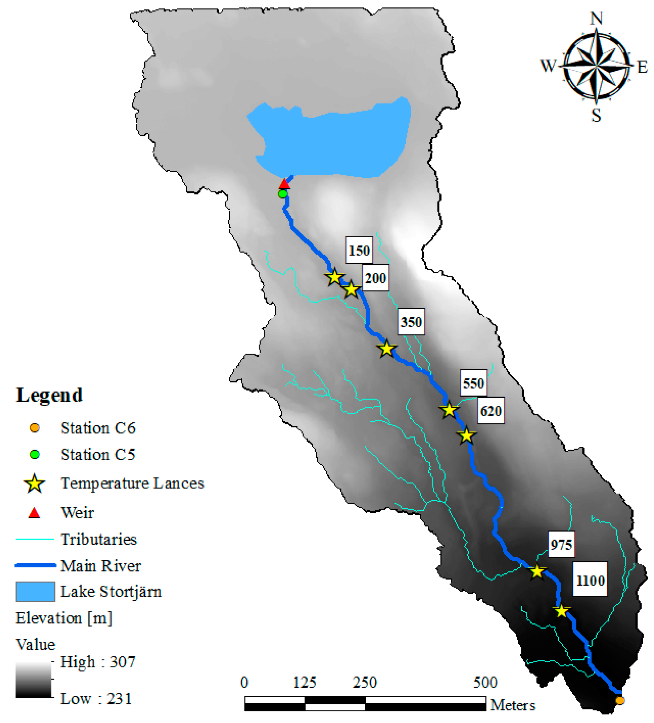
The current study focused on a stretch of river with a length of approximately 1500 m, delimited by two hydrological stations, namely C5 and C6, in the upstream and downstream regions, respectively. Lake Stortjärn is located 100 m upstream of station C5. The lake has an area of 4 ha and is fed by a mire system. The river stretch can be considered as the gaining stream in which the stream water source is dominated by Lake Stortjärn. However, there are several parts of the stream segment with losing condition which is highly controlled by topography. The subcatchment area draining the stretch of river between stations C5 and C6 is mostly covered by forest containing Scots pine (Pinus sylvestris), Norway spruce (Picea abies), and birch (Betula pubescens). Peat dominates the riparian zones of the river stretch in which organic content increases in riverbanks. Streambed sediment type varies along the river, and includes dense decomposed organic matter, sand, and cobble/boulder [44]. The width of the stream channel between stations C5 and C6 varies between 0.3 and 2 m, and the average slope of the stream is approximately 3% [46]. Figure 1 shows the subcatchment of the Krycklan Catchment Study (KCS) area in which the experiment was carried out.
2.2. Field Measurement
During the experiment, the outflow from Lake Stortjärn into the stream discharge was regulated to simulate high and low downstream flow discharges. The regulation was conducted by closing a gate of a V-notch weir located approximately 50 m downstream of the lake outlet (Figure 1). The V-notch weir was completely closed during the period of 07–24 August 2017 so that no water entered the stream from Lake Stortjärn. Water was pumped downstream of the (closed) weir to simulate a high-flow pulse on 19 August (07:22 until 18:17) and 21 August (06:15 until 09:07) of 2017.
Leach et al. [44] delineated a set of upwelling and downwelling zones between stations C5 and C6. Vertical temperature profiles were recorded at seven locations along the stream reach. Starting from upstream, vertical temperature profiles were recorded at distances of 150, 200, 350, 550, 620, 975, and 1100 m from the outflow of Lake Stortjärn (Figure 1). Temperatures were recorded by means of Multi-Level Temperature Sticks (MLTS; UIT, Dresden, Germany) [47]. The MLTS sticks are polyoxymethylene probes featuring eight TSIC-506 thermometer sensors located at various distances from the head of the lance (i.e., the upper part), namely −60, −35, −25, −20, −15, −10, −5, and 0 cm. At the location 975 m from the outflow of the lake, a longer temperature stick was deployed with sensors located at −83, −65, −48, −31, −23, −17, −13, and 0 cm from the head of the lance. Each temperature sensor recorded at a temporal resolution of 5 min. The measuring range of the temperature sensors was between 5 and 45 °C, with a resolution of 0.04 °C. The typical accuracy of the sensors was 0.07 °C. Temperature sticks were hammered into the streambed on 3 August.
Stream discharge was continuously recorded at both the upstream (C5) and downstream (C6) stations at a temporal resolution of 1 min. Five different times of year were chosen in order to capture the intra-annual variability of the hydrological response of the catchment, namely, 22 May 2017 (snow melt flow), 27 June 2017 (summer base flow), 18 August 2017 (low flow), 19 August 2017 (high flow), and 30 August 2017 (autumn base flow). The stream discharge along the main channel was estimated for each of the aforementioned flow discharges (i.e., snow melt, summer, low, high, and autumn flows) at a spatial resolution of 50 m, accounting for the progressive downstream drainage area (Table 1 and Figure S1 in the Supplementary Materials). Moreover, the mean water depth of the river was measured at a spatial resolution of 50 m for each of the five mentioned flow discharges (Table 1). It should be mentioned that the mean water depth for summer flow was only measured up to 400 m from the upstream station.
2.3. Field Data Analysis
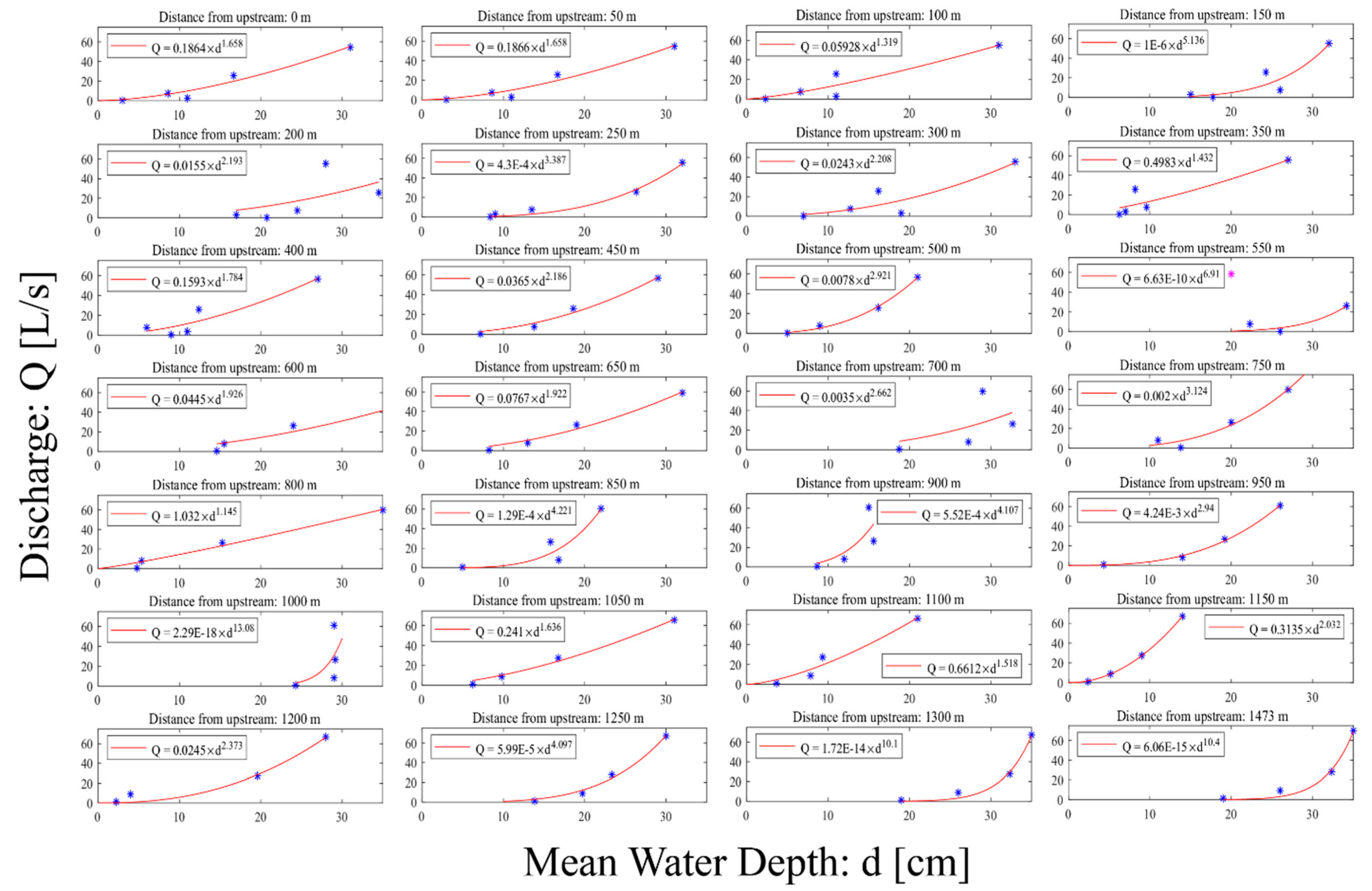
A power-law relationship was established between stream discharge estimates (Table 1) and measured water depths (Table 1) at a spatial resolution of 50 m along the stream. The power-law relationship provides the means for estimation of water depth with the spatial resolution of 50 m for low-, high-, and base-flow condition using the measured discharge intensities. Figure 2 (and Table S1 in the Supplementary Materials) shows the rating curves that were calculated for each specific location along the stream. The rating curves were used to determine the water depths which subsequently were used as the boundary condition on the streambed interface of the numerical model.
The experimental period (03–21 August) was divided into subperiods reflecting base-, low-, and high-flow discharges (Table 2). The mean stream discharge at a spatial resolution of 50 m along the main channel was estimated for each of the three aforementioned flow discharges accounting for the progressive downstream drainage area. Finally, the corresponding water depth for each flow discharge was estimated using the estimated discharge and correlation functions shown in Figure 2 at a spatial resolution of 50 m (Table S2 in Supplementary Materials). These water depths were later used (Section 2.3) to address the top boundary condition of the numerical model for base-, low-, and high-flow discharges.
2.4. Modeling Framework
The numerical model was developed using the COMSOL Multiphysics® software to simulate a two-dimensional longitudinal transect along the center of the stream network. The Brinkman–Darcy equation (Equation (1)) was used with the continuity equation to describe the subsurface flow in the hyporheic zone near the streambed surface:
where ρ [kg/m3] is the water density, ε [–] is the Brinkman porosity, u [m/s] is the subsurface velocity vector, t [s] is the time, p [pa] is the water pressure, μ [pa.s] is the water’s dynamic viscosity, μe [pa.s] is the water’s effective viscosity, k [m2] is the intrinsic permeability of the sediment, and ( is the Darcy term.
In the present study, the subsurface flow model includes Quaternary deposits, in which the top surface was quantified using a digital elevation model (DEM) file representing the stream morphology with a resolution of 50 cm. The depth of the Quaternary deposits varies along the stream, and is up to 17 m [48].
In order to investigate the effect of hydrogeological properties on the hyporheic flow fields, flow simulations were performed using two different sediment permeability scenarios: (a) constant permeability; and (b) depth-decaying permeability. The first permeability scenario was performed using a constant intrinsic permeability (k = 10−9 [m2] representing the streambed sediment [18]) for the entire subsurface region. The second permeability scenario was performed by applying a decaying intrinsic permeability in the top meter of the subsurface region (starting with k = 10−9 [m2] for the top surface decaying to k = 10−12 [m2] at a depth of 1 m) and a constant intrinsic permeability (k = 10−12 [m2] refers to the glacial sediment soil type) for the rest of the subsurface region (deeper than 1 m from the top surface). The depth-decaying function for the soil permeability was defined based on the findings of Morén et al. [18]. They performed an experiment in a small stream in Sweden (Tullstorps Brook) and measured the hydraulic conductivity at two depths (i.e., 3 and 7 cm) every 100 m for a reach of 1500 m. The permeability k(z) of the top meter of the stream was described according to [17]:
where k0 [m2] is the intrinsic permeability at the streambed interface, z [m] is the depth from the streambed, and c [m−1] is an empirical decay coefficient. An exponential function was fitted to the measured data of Morén et al. [18] with a lower hydraulic conductivity limit of K = 10−6 [m/s] (corresponding to an intrinsic permeability of k = 10−12 [m2]) for a depth of 1 m from the streambed surface (Figure S2, Supplementary Materials).
The numerical model was constructed using a computational mesh with a non-uniform size and an increasing resolution at depths ranging between 0.03 and 14 m. The mesh size formation in longitudinal direction (along the stream) depends on streambed morphology fluctuation. The more morphology fluctuation, the lower mesh size.
A pressure boundary condition was assigned based on the surface flow discharge. In particular, a hydrostatic pressure was applied at the sediment interface based on the overlying water depths estimated as described in Section 2.3 (Table S2 in the Supplementary Materials). The spatially varying head boundary condition at the streambed surface was calculated by: , where [pa] is the pressure distribution at the streambed topography surface, g [m/s2] is the gravitational acceleration, and [m] is the water depth for each flow discharge. The water depth was quantified using the corresponding mean discharge value for each flow discharge (see Section 2.3). Furthermore, an open boundary was assumed for the upstream and downstream sides, whereas a no-flow boundary was considered for the bottom surface of the model. Each model was run to a steady state flow condition based on hydrostatic head boundary condition on the top surface.
The flow velocities at the streambed interface, as well as trajectories and residence times of 1000 uniformly distributed water particles at the streambed water interface, were evaluated during the three types of flow discharge (i.e., base-, low-, and high-flow discharges). It should be noted that the movement of the streambed sediment was not accounted for in the numerical model. The hyporheic exchange depth, hyporheic flux residence times, and the fragmentation of upwelling length were considered as the metrics. Fragmentation quantifies the heterogeneity in the spatial distribution of the zones characterized by gaining and losing behavior [15]. In particular, fragmentation is defined as the size distribution of spatial coherent upward and downward lengths. Here, the frequency of occurrence of different lengths of coherent upwelling and downwelling regions at the streambed interface was represented by a cumulative distribution function (CDF). An increase in the fragmentation of coherent flow regions results in a shift towards shorter (upwelling/downwelling) lengths in the CDF plot. It should be mentioned that this definition is independent of the magnitude of the fluxes.
3. Results
3.1. Water Temperature
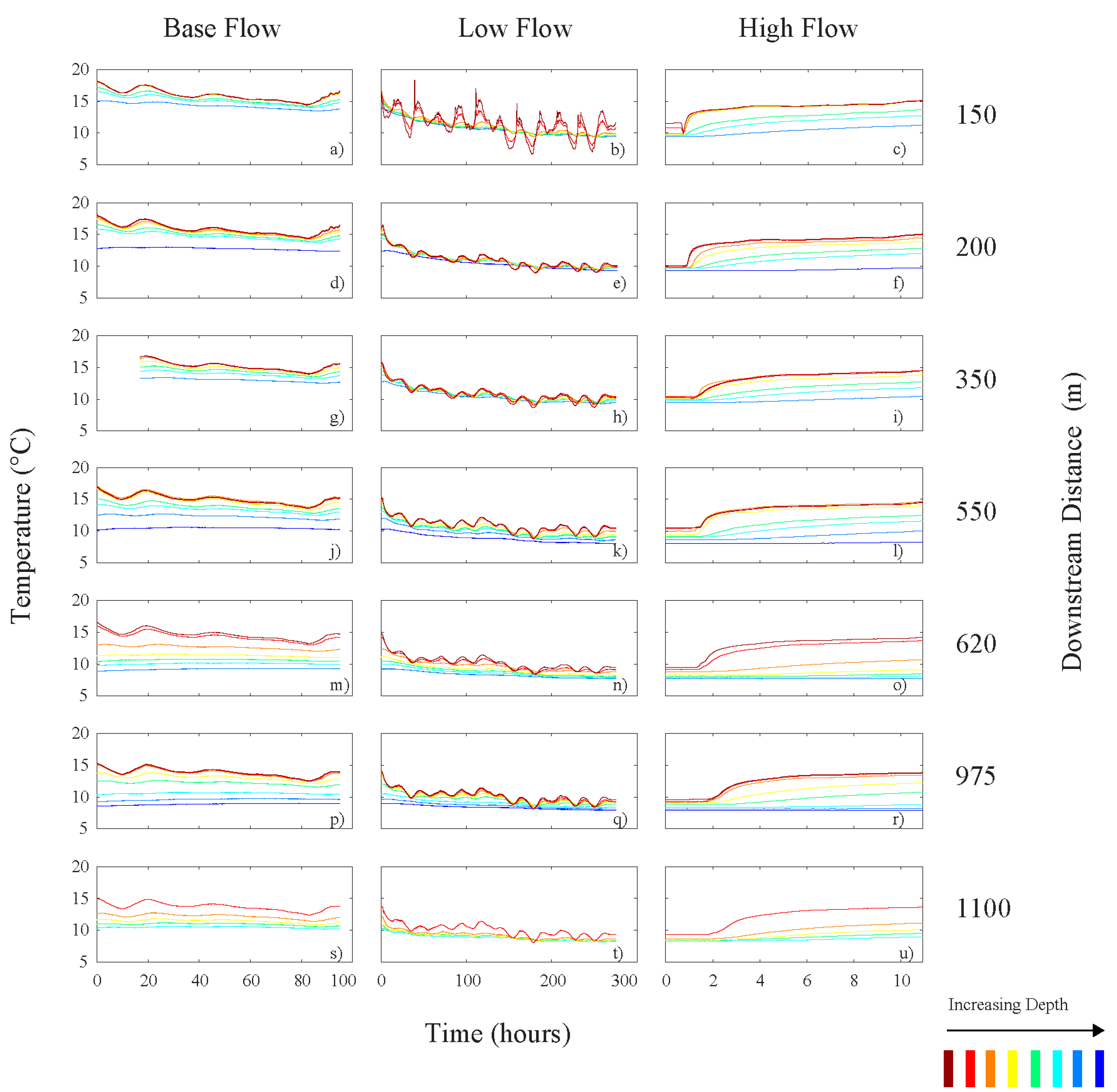
Time series of the measured water temperature at the seven monitoring locations for the different flow discharges (i.e., base-, low-, and high-flow) are presented in Figure 3. Each time series corresponds to the temperature recorded by sensors at increasing depth. Note that the period of record (i.e., the horizontal axis for each column in Figure 3) differs between the three flow regimes, with the low-flow and high-flow discharges having the longest and shortest records, respectively. Since no full diurnal cycles are captured during high-flow discharge (the recorded time period is about 10 h), the variability of the temperature signals is smaller compared to the high- and base-flow discharges. On the other hand, low-flow discharge displays larger temperature fluctuations at shallower depths compared to the base-flow discharge. Temperature lances located at distances of 150, 200, and 350 m from the upstream station recorded a relatively wider range of temperature for the base-flow discharge than the high-flow discharge; conversely, the difference in temperature distribution was negligible between the different flow discharges for temperature lances located at 550, 620, 975, and 1100 m. During high-flow discharge, all temperature time series clearly highlight the moment when the flood wave reaches each location (temperature increments are delayed at further downstream locations).
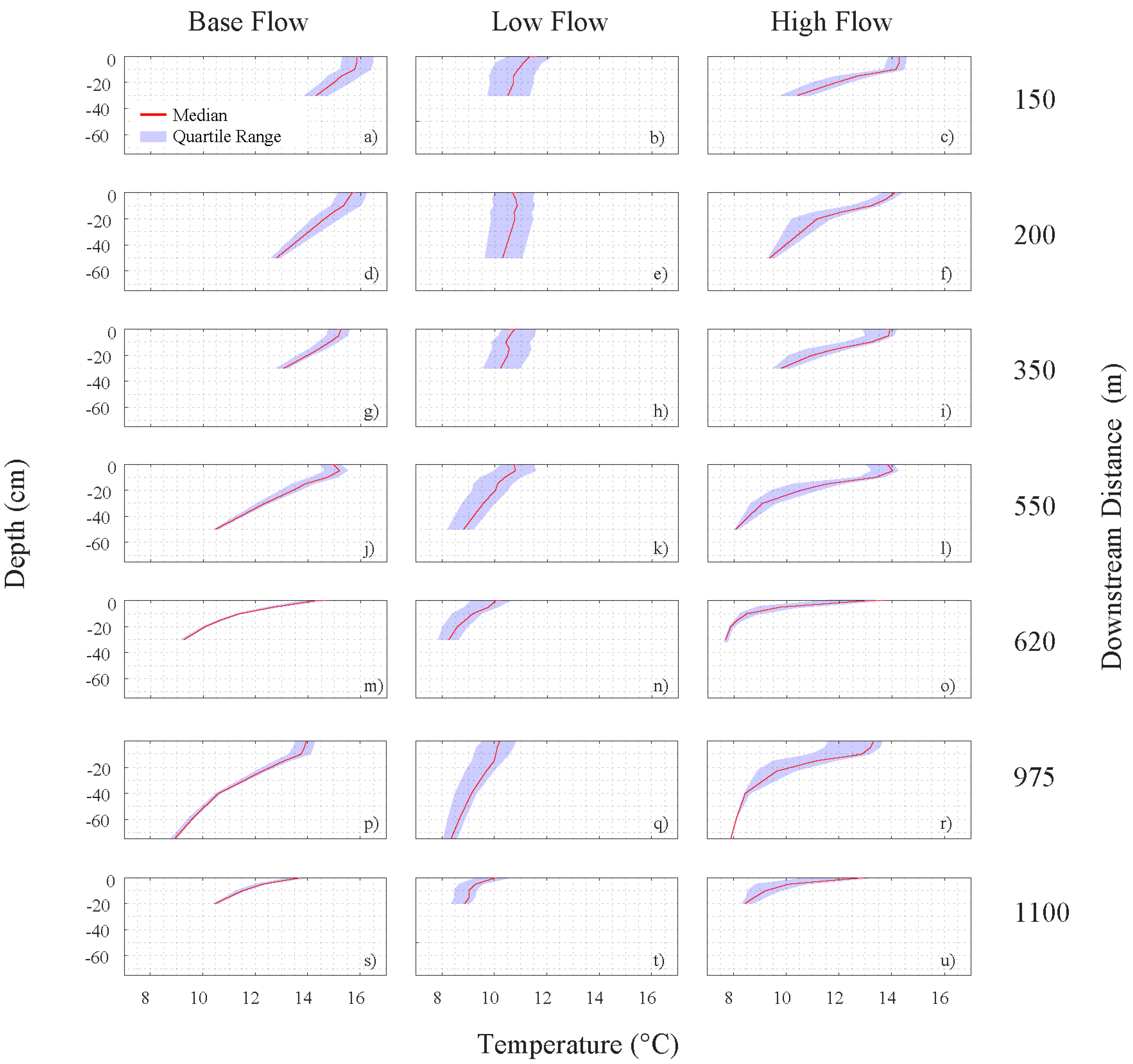
Figure 4 shows the temperature envelopes versus depth for all monitoring locations during the three different flow discharges. The envelopes represent the median and the interquartile range of the temperature signals. The statistics were evaluated for each sensor (i.e., for each depth) during different flow discharges. Median and quartiles were then linearly interpolated between the sensors. The envelopes effectively show the temperature pattern with increasing depth as well as the vertical variability of the temperature signal. Steep gradients of median temperature suggest an abrupt transition between higher surface-water temperatures and lower groundwater temperatures. This generally indicates cold upwelling fluxes approaching the surface of the streambed and, consequently, suggests the existence of shallow hyporheic zones. Strong temperature gradients with increasing depth are generally associated with decreased spatial variability in the temperature signal (i.e., a narrow interquartile range). This is a consequence of the relatively constant temperature of groundwater throughout the year (in the range of 8–12 °C), in contrast to the strong temporal dynamics of surface water temperature. The results indicate that low-flow discharge has the lowest temperature range (8–12 °C) and the base-flow discharge has the highest temperature range (9–16 °C). Additionally, the variability of the temperature envelope with depth for different flow discharges shows a similar behavior at distances of 150, 200, and 350 m from the upstream station, while the behavior at distances of 550, 620, 975, and 1100 m are similar to each other but different from those of the other flow group. It should be noted that, in case of base- and low-flow discharges, daily cycles in surface water temperature are mostly responsible for the variability in temperature envelopes (represented by the quartile range in Figure 4). On the other hand, the observed variability in temperatures during high-flow discharge is a consequence of the abrupt increment of temperature that is experienced at all motoring locations at the arrival of the flood wave.
3.2. Modeling Results
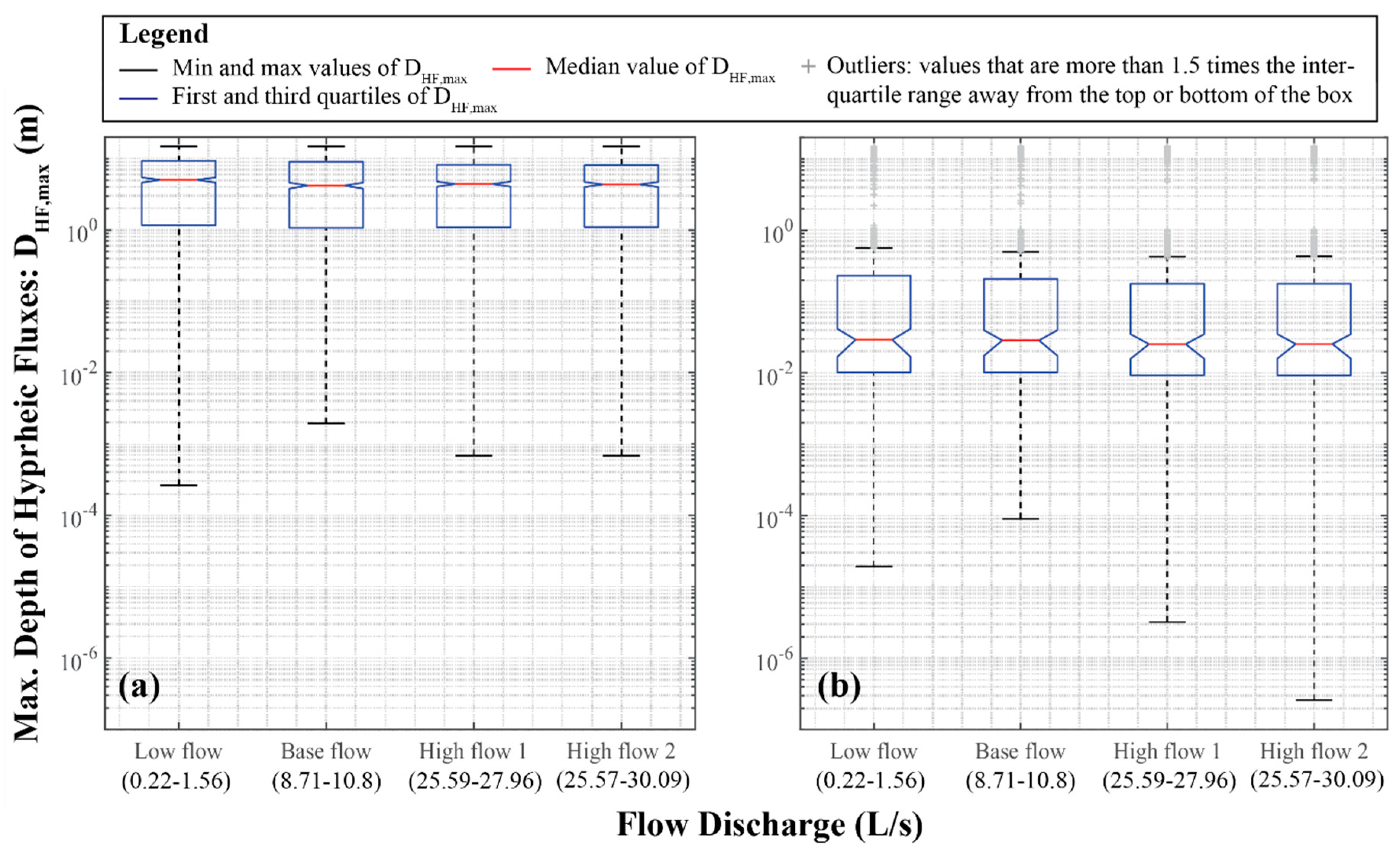
The hyporheic flow field was quantified for the study reach. The spatial distribution of the maximum depth of the hyporheic fluxes was quantified based on the deepest point of the streamlines (DHF,max). Figure 5 shows the calculated maximum depths of the hyporheic fluxes for the case of constant permeability (Figure 5a) and decaying permeability in the top meter of the flow domain (Figure 5b). The results indicate that DHF,max varied during the three flow discharges. In particular, the minimum DHF,max is highly affected by stream water flow intensity (the range of DHF,max is affected by the order of 10 and 100 in constant and decaying permeability scenarios, respectively). High-flow discharges have lower values of DHF,max than the base-flow discharge, whereas the minimum DHF,max for the base flow is higher than that for low-flow discharge, regardless of the permeability scenario applied. The median value of DHF,max varies slightly between different flow discharges, with the low-flow discharge having the highest median value of DHF,max among all the flow discharges, i.e., 4 m and 0.03 m in constant and decaying permeability scenarios, respectively (Figure S3 in the Supplementary Materials). However, in the case of decaying permeability, the median value of DHF,max (Figure 5b) is in the range of centimeters which is substantially lower than in the constant permeability case (Figure 5a) that is in a range of meters. Additionally, the logarithmic ranges of interquartile of the maximum depth of the hyporheic fluxes in the constant permeability case (Figure 5a) are smaller than those in the decaying permeability scenario (Figure 5b) for all flow discharges.
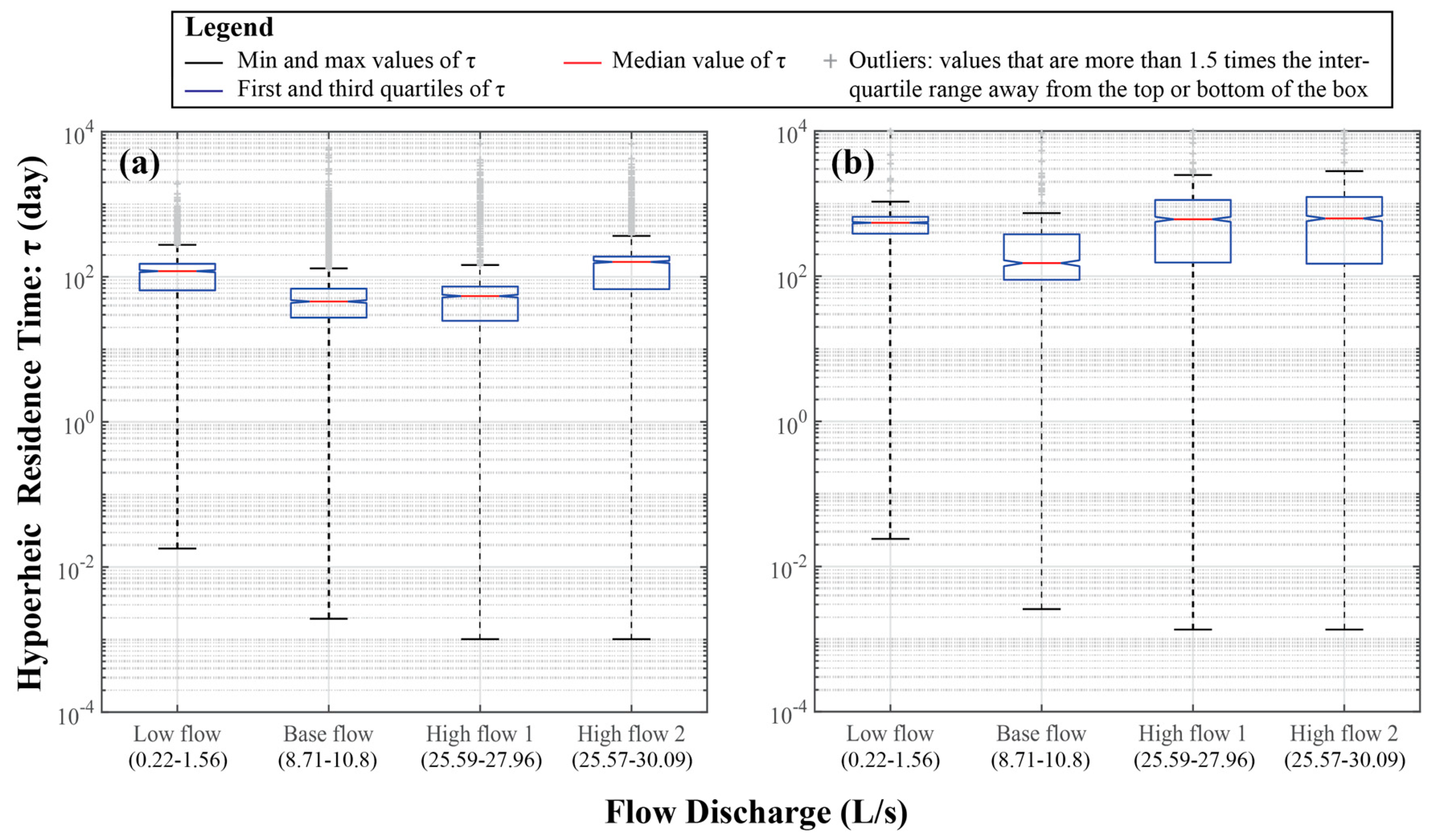
The second metric that was analyzed was the residence time of each released particle at the streambed interface. In this study, the residence time is defined as the time taken for the water to enter along a streamline through the streambed and return to the streambed surface again. Figure 6 presents the distribution of residence times for 1000 water parcels that were uniformly distributed at the streambed surface. In both permeability cases (i.e., decay and no decay), the high flow discharges have a larger range of residence times. The minimum residence time varies among different streamflow discharges, with increasing flow discharge intensity resulting in the decrease of the minimum hyporheic flow residence time. The influence of permeability is evident in the interquartile ranges of residence time. A vertical gradient of permeability induces a larger interquartile range of residence times (i.e., a larger variability in residence times). Additionally, the decaying of permeability results in a higher median value of residence time compared to the homogeneous case, i.e., in the order of 10 (Figure 6a,b).
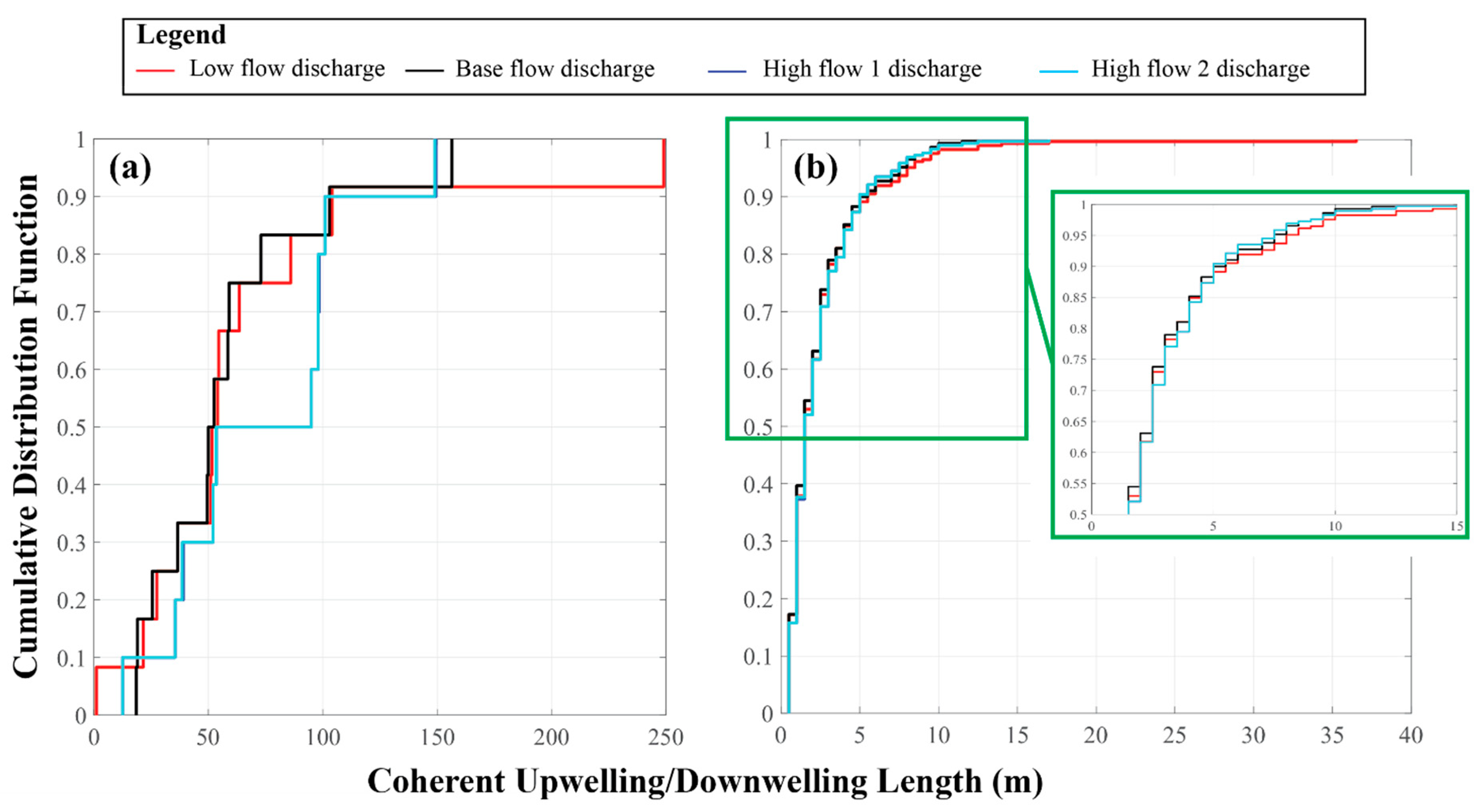
Finally, the velocity field at the streambed interface was analyzed with a spatial resolution of 50 cm in order to investigate the distribution of coherent upwelling zones (i.e., lengths of upwelling zones) for different flow discharges. The CDF of the length of the coherent upwelling was computed. The results indicate that applying a decaying permeability function strongly influences the fragmentation of hyporheic flows (Figure 7). Considering a constant permeability for the whole subsurface (Figure 7a) results in significant variation in the fragmentation length between different flow intensities, with the high-flow discharges being less fragmented (larger upwelling/downwelling lengths) than the other flow discharges. In this case, for almost 90% of the lengths, the base flow and low flow are the most fragmented flows. On the other hand, assuming a depth-decaying permeability induces a similar fragmentation of coherent upwelling length for all the flow discharges (Figure 7b). However, in this case, the hyporheic exchange during low-flow discharge is less fragmented at lengths larger than 5 m compared to the other flow discharges.
4. Discussion
A comprehensive understanding of the impacts of flow discharge on hyporheic exchange fluxes is essential to highlight the effect of streamflow dynamics on the extent of hyporheic exchange. Here, we combined field experiments with numerical modeling to estimate the variation in hyporheic depth and flow velocity field in a boreal stream.
4.1. Temperature Variation in the Streambed Sediment
The experiment of the present study was performed in summer, when groundwater is colder than stream water. Hence, the diurnal fluctuation of stream water temperature can be used to investigate the hyporheic exchange and identify gaining and losing reaches [49]. During summer, the water temperature of the hyporheic zone tends to decrease as the depth of the streambed increases [50]. At the same time, the stream water temperature signal is progressively damped at larger depths. These effects result from mixing between deep cold subsurface water and warm surface water mediated by the thermal dispersion associated with both thermal diffusion and hydrodynamic dispersion [25]. However, this general trend displays significant variations between monitoring locations as well as during different flow discharges (Figure 3). The temperature time series indicates areas of upwelling and of downwelling in the experimental reach. Strong downwelling conditions can be observed both in large and relatively erratic temperature records (e.g., at a distance of 150 m from the outflow of Lake Stortjärn for the base-flow discharge) and by observing the surface temperature dynamics at larger depths (e.g., at a distance of 150, 200, and 350 m from the outflow of Lake Stortjärn for low-flow discharges). A milder downwelling condition is suggested when the recorded temperature at greater depths is significantly larger than the average groundwater temperature (at a distance of 200 and 350 m from the outflow of Lake Stortjärn for the base-flow discharge), which suggests advective downward fluxes. The increase in temperature at larger depth during the high-flow discharge also suggests mild downwelling fluxes (at a distance of 350 m from the outflow of Lake Stortjärn for high-flow discharge). On the other hand, the relatively large difference in average temperature with increasing depth suggests areas of upwelling (at a distance of 550, 620, 975, and 1100 m from the outflow of Lake Stortjärn).
During low-flow discharge, the sediments in downwelling reaches are likely to experience reduced saturation, facilitating thermal diffusion towards deeper soils (due to lower thermal inertia) [51]. However, the lack of significant surface water fluxes during low-flow discharge hinders the interpretation of temperature data. Thermal diffusion can play a major role in sediment heat transfer, and its relation with soils having heterogeneous saturation can significantly complicate the analysis of temperature data. In general, the similarity of the temporal variation in temperature and the difference in temperature at different depths indicate upwelling and downwelling conditions in the stretches. A higher temperature at depth indicates a more robust downwelling condition, whereas a larger difference in temperature at depth shows upward fluxes.
The temperature envelopes shown in Figure 4 tend to confirm upwelling and downwelling stretches result as is suggested by temperature time series. Moreover, they can be used to further interpret the spatial patterns of hyporheic exchanges under the different flow discharges.
Under the base-flow discharge, the locations 150 and 200 m from the outflow of Lake Stortjärn (and to some extent 350 m) display clear signs of downwelling conditions. The gradient in the median temperature is lower than in the remaining sites, and the temperature is variable at greater depths. This suggests a significant convective heat transport following surface water flows towards deeper soil layers. Conversely, the strong vertical temperature gradients, together with the narrow interquartile ranges of temperature, confirm upwelling conditions at the locations 620 and 1100 m from the outflow of Lake Stortjärn (Figure 4m,s). Additionally, moderate upwelling conditions and the development of a shallow hyporheic zone are suggested by the small variability of temperature with depth observed at locations 550 and 975 m from the outflow of Lake Stortjärn.
As already mentioned, the temperature data under low-flow discharge is more complex than for the other flow discharges. In the low-flow discharge condition, the hyporheic flow at downwelling locations does not only include direct downwelling from the surface water, but can also include the upwelling of hyporheic water (e.g., water that has infiltrated upstream). On the other hand, the signature of groundwater upwelling might be more easily detectable, since large groundwater circulation patterns can be less affected by streamflow discharges. At low-flow discharge, temperature envelopes can be divided into two groups: the first includes the locations 150, 200, and 350 m from the outflow of Lake Stortjärn, and the second includes the remaining downstream sites. In the first three upstream locations, the median temperature remains almost constant as the depth in the streambed sediments increases. Furthermore, the temperature variability (represented by the interquartile range) remains stable across depth, while featuring extremely large values. The undisturbed propagation (i.e., small damping) of the temperature signal at larger depths suggests a reduced thermal inertia of the sediments during low-flow discharges. This may be related to unsaturated conditions established in the sediments during this phase. The establishment of unsaturated conditions further suggests the absence of significant groundwater flow in these locations.
The temperature envelopes at the remaining downstream locations (i.e., 550, 620, 975, and 1100 m from the outflow of Lake Stortjärn) display a different pattern. As depth increases, temperature decreases, both in terms of median temperature and interquartile range. Moreover, the temperatures measured at the surface are lower compared to those at the first three upstream locations. This is likely a consequence of groundwater upwelling.
Moreover, during the high-flow discharge, a significant increase in surface temperature is observed at all locations. At locations 150, 200, and 350 m from the outflow of Lake Stortjärn, the vertical temperature gradient increases compared to the base-flow discharge, suggesting the development of a hyporheic zone with a reduced extent. The inflection of the median temperature profile at sites 550 and 975 m from the outflow of Lake Stortjärn (Figure 4l,r) suggest a shallow (i.e., 10–20 cm in depth) hyporheic zone. The enhanced exchange of surface water with sediments is further suggested by the increased variability in the temperature profile compared with the base-flow discharge. On the other hand, the large temperature gradient at locations 620 and 1100 m from the outflow of Lake Stortjärn suggests significant upwelling fluxes, possibly reinforced by pressure gradients triggered by high flow discharges.
Our experimental findings regarding the regions of upwelling and downwelling confirm the experimental results of Leach et al. [44], who estimated gaining regions using distributed temperature sensing (DTS) fiber-optic cable. A comparison of the base- and high-flow discharges in Figure 4 reveals a higher contribution of stream water than groundwater in the hyporheic zone for high-flow discharge. Increasing the stream water flow discharge increases the variability of the hydrostatic pressure distribution on the streambed interface; hence, the hyporheic flow gradient is increased, which overwhelms the groundwater flow gradient. Consequently, the penetration depth increases, which increases the depth of the hyporheic zone.
4.2. The Role of the Heterogeneity of Sediment Permeability in Hyporheic Exchange
The complex pattern of temperature distribution observed in the field suggests an enhanced spatiotemporal variability of hyporheic flows. The implementation of the numerical model presented in Section 2.3 aims to capture the reach-scale flow patterns highlighted by the analyses of the temperature data collected in the field. The role of the heterogeneity of streambed sediment was investigated due to its strong impact on the distribution of hyporheic flow paths [52,53]. In particular, the effect of depth-decaying permeability on hyporheic fluxes was investigated in this study. As expected, the stream water penetrates into deeper sediment in the case of constant intrinsic permeability (Figure 5a), while the hyporheic zone is much shallower in the case of depth-decaying permeability (Figure 5b). This is basically due to the shielding effect of decreasing permeability with depth [8]. Low permeability sediment acts as a semi-impermeable surface that inhibits the penetration of stream water into deeper sediment. The high-flow discharge has a relatively shallower median hyporheic zone (Figure S3). The reason for this is the lower variability in the spatial gradient of the hydrostatic hydraulic head during high-flow discharges than during low- and base-flow discharges, at least for part of the study reach. The minimum and median values of hyporheic depth vary slightly between high flow 1 and 2 due to the slight change in the stream water flow discharge between these conditions (Table 2).
The results of this study indicate that increasing the flow discharge results in a larger distribution of hyporheic residence time. High-flow discharges cause a longer flow path, which consequently increases the residence time. On the other hand, the hyporheic fluxes with long residence time act like groundwater flow at upwelling reaches, so that stream water is prevented from penetrating into the sediment. This leads to a short flow path as well as a short residence time of hyporheic flow [38]. Therefore, upwelling and downwelling regions control the behavior of the residence time, with short residence times corresponding to upwelling zones and long residence times corresponding to the hyporheic fluxes starting their journey into the sediment from downwelling regions. The results of this study regarding hyporheic depth and residence time confirms the finding of Cardenas et al. [52] regarding the large dependency of the hyporheic flow process on the heterogeneity of streambed permeability.
Mojarrad et al. [15] observed variation in the fragmentation of coherent upwelling and downwelling zones for different stream orders (i.e., stream water depths). They found that the fragmentation of upwelling zones can vary depending on the large-scale groundwater contribution. However, the variation in the fragmentation of downwelling zones was negligible as there was no groundwater contribution in these areas. Mojarrad et al. [15] showed that increasing the stream order decreased the fragmentation of coherent upwelling zones but did not influence the fragmentation of coherent downwelling areas, which is consistent with our findings. In the present study, it was found that, in the case of a homogeneous subsurface, the stream water can penetrate the whole depth of the Quaternary deposits. Hence, the impact of a deeper flow streamline should be observed in the fragmentation length. As is shown in Figure 7a, high-flow discharges (i.e., a higher stream depth) are less fragmented compared to the low- and base-flow discharges. This is due to the effect of deeper flow on upwelling zones. On the other hand, Mojarrad et al. [15] showed that the fragmentation of downwelling zones varies slightly with stream order if the contribution of deep groundwater is negligible. Depth-decaying permeability prevents the deep penetration of stream water into the stream sediment, which is similar to the finding of Mojarrad et al. [15] that groundwater does not contribute to hyporheic fluxes in downwelling zones. Therefore, in this study, the fragmentation of upwelling areas differs slightly between flow discharges.
Field experiments consist of all the parameters that influence the hyporheic exchange. Heterogeneity in permeability of subsurface sediment is one of the factors that significantly controls the upwelling and downwelling regions, as well as the depth of hyporheic zone. Here, the result of field experiment showed that depth of hyporheic zone vary up to 50 cm in different flow discharges (Figure 4). This result confirms the numerical model results with the decaying intrinsic permeability. It was indicated that assuming homogeneous subsurface leads to hyporheic depth in the order of meters, whereas applying decaying in subsurface permeability results in much shallower hyporheic zone with the maximum depth of 40–60 cm (Figure 5). This result confirms the critical role of heterogeneity in subsurface flow, which should be considered in numerical modelling to improve the understanding of hyporheic flow processes.
5. Conclusions
This study investigated the impact of different stream discharges on the hyporheic zone using experimental and numerical approaches. We measured streambed temperature profiles at different locations along a boreal stream in northern Sweden. Different streamflow discharges were investigated by pumping water into the stream channel over a blocked weir. A numerical model was applied to investigate the impact of stream discharge on hyporheic exchange using geomorphological and hydrological data for the experimental reach. The gaining and losing conditions were evaluated using temperature data for the streambed sediment. In particular, this study evaluated locations of strong downwelling (at distances of 150, 200 m from the outflow of Lake Stortjärn), mild downwelling (at distances of 350 m from the outflow of Lake Stortjärn), mild upwelling (at distances of 550 and 975 m from the outflow of Lake Stortjärn), and strong upwelling (at distances of 620 and 1100 m from the outflow of Lake Stortjärn). The results show that increasing flow discharge increases hyporheic depth through the development of nested hyporheic flow paths. The contribution of groundwater to surface water is larger during low-flow discharge than during high-flow discharge, which is manifested as higher temperatures in the stream water. The modeling results agree with the experimentally measured temperature, showing a deeper penetration of stream water into sediment during high-flow discharges. Additionally, increasing streamflow discharge results in a larger distribution of the residence time of hyporheic fluxes. This is more evident in residence time distributions in which the high-flow discharges display larger interquartile ranges. Furthermore, the modeling results highlight the fact that heterogeneity in the permeability of the streambed sediment strongly controls the hyporheic flow exchange. The fragmentation of coherent upwelling length was defined as the shift of the CDF towards shorter lengths. The fragmentation of coherent upwelling length varied with streamflow discharge, with high-flow discharges being less fragmented. When permeability decayed with depth, flow paths were constrained to shallow regions; consequently, the upwelling fluxes were reduced and the fragmentation of the upwelling length was less variable between different flow discharges.
Supplementary Materials
The following are available online at https://www.mdpi.com/2073-4441/11/7/1436/s1, Figure S1: “Map showing the draining area every 50 m along the main river of the subcatchment, as well the main river (dark blue color), tributaries (light blue color), the lake Stortjärn (solid light blue region), and 50 m distance markers (red dots) from upstream”, Figure S2: “Hydraulic conductivity decay function along the depth. Red color dashed lines represent the measured values from Morén [18], and blue color solid line is the mean exponential function for all the measured data”, Figure S3: “Mean value of hyporheic zone depth under various flow condition assuming: (a) constant intrinsic permeability (k = 10−9 [m2]) for the entire subsurface region and (b) decaying intrinsic permeability (starting from k(z = 0) = 10−9 [m2] at the surface–subsurface water interface and decaying exponentially to k(z = –1) = 10−12 [m2] down to a depth of 1 m). In the case of vertically varying permeability, a constant permeability (k = 10−12) was used for depths larger than 1 m.”, Table S1: “Correlation between discharge and mean water depth using five flow data for every 50 m distance from upstream along the main river”, Table S2: “Estimated mean water depth for different flow condition every 50 m from upstream”.
Author Contributions
Conceptualization, B.B.M.; Investigation, B.B.M., A.B., and C.O.; Methodology, B.B.M.; Formal Analysis, A.B., and B.B.M.; Project Administration, B.B.M.; Software, B.B.M., and T.S.; Visualization, B.B.M., and A.B.; Writing—original draft preparation, B.B.M., A.B., and T.S.; Writing—review and editing B.B.M., A.B., C.O., and A.W., Supervision A.W.; Funding Acquisition A.W.
Funding
This project was supported by the EU’s Horizon 2020 Research and Innovation Programme under Marie-Skłodowska-Curie grant agreement No. 641939 and the Swedish Radiation Safety Authority, SSM.
Acknowledgments
We would like to thank Anna Lupon (CEAB-CSIC); Nicolai Brekenfeld, University of Birmingham; and the crew of Krycklan Catchment Study (KCS) funded by SITES (VR), for their help in the field campaign.
Conflicts of Interest
The authors declare no conflict of interest.
References
- Cardenas, M.B. Hyporheic zone hydrologic science: A historical account of its emergence and a prospectus. Water Resour. Res. 2015, 51, 3601–3616. [Google Scholar] [CrossRef]
- Tonina, D.; Buffington, J.M. Effects of stream discharge, alluvial depth and bar amplitude on hyporheic flow in pool-riffle channels. Water Resour. Res. 2011, 47. [Google Scholar] [CrossRef]
- Stanford, J.A.; Ward, J.V. The hyporheic habitat of river ecosystems. Nature 1988, 335, 64–66. [Google Scholar] [CrossRef]
- Sawyer, A.H.; Bayani Cardenas, M.; Buttles, J. Hyporheic temperature 165 dynamics and heat exchange near channel-spanning logs. Water Resour. Res. 2012, 48. [Google Scholar] [CrossRef]
- Harvey, J.W.; Böhlke, J.K.; Voytek, M.A.; Scott, D.; Tobias, C.R. Hyporheic zone denitrification: Controls on effective reaction depth and contribution to whole stream mass balance. Water Resour. Res. 2013, 49, 6298–6316. [Google Scholar] [CrossRef]
- Boano, F.; Camporeale, C.; Revelli, R.; Ridolfi, L. Sinuosity-driven hyporheic exchange in meandering rivers. Geophys. Res. Lett. 2006, 33. [Google Scholar] [CrossRef]
- Elliott, A.H.; Brooks, N.H. Transfer of nonsorbing solutes to a streambed with bed forms: Theory. Water Resour. Res. 1997, 33, 123–136. [Google Scholar] [CrossRef]
- Gomez-Velez, J.D.; Krause, S.; Wilson, J.L. Effect of low-permeability layers on spatial patterns of hyporheic exchange and groundwater upwelling. Water Resour. Res. 2014, 50, 5196–5215. [Google Scholar] [CrossRef] [Green Version]
- Stonedahl, S.H.; Harvey, J.W.; Packman, A.I. Interactions between hyporheic flow produced by stream meanders, bars, and dunes. Water Resour. Res. 2013, 49, 5450–5461. [Google Scholar] [CrossRef]
- Sawyer, A.H.; Cardenas, M.B.; Bomar, A.; Mackey, M. Impact of dam operations on hyporheic exchange in the riparian zone of a regulated river. Hydrol. Process. 2009, 23, 2129–2137. [Google Scholar] [CrossRef]
- McGlynn, B.L.; McDonnell, J.J.; Shanley, J.B.; Kendall, C. Riparian zone flowpath dynamics during snowmelt in a small headwater catchment. J. Hydrol. 1999, 222, 75–92. [Google Scholar] [CrossRef]
- Malcolm, I.A.; Soulsby, C.; Youngson, A.F.; Petry, J. Heterogeneity in ground water–surface water interactions in the hyporheic zone of a salmonid spawning stream. Hydrol. Process. 2003, 17, 601–617. [Google Scholar] [CrossRef]
- Schmidt, C.; Bayer-Raich, M.; Schirmer, M. Characterization of spatial heterogeneity of groundwater-stream water interactions using multiple depth streambed temperature measurements at the reach scale. Hydrol. Earth Syst. Sci. Discuss. 2006, 3, 1419–1446. [Google Scholar] [CrossRef] [Green Version]
- Boano, F.; Revelli, R.; Ridolfi, L. Reduction of the hyporheic zone volume due to the stream-aquifer interaction. Geophys. Res. Lett. 2008, 35, L09401. [Google Scholar] [CrossRef]
- Mojarrad, B.B.; Riml, J.; Wörman, A.; Laudon, H. Fragmentation of the hyporheic zone due to regional groundwater circulation. Water Resour. Res. 2019, 55, 1242–1262. [Google Scholar] [CrossRef]
- Saar, M.O.; Manga, M. Depth dependence of permeability in the Oregon Cascades inferred from hydrogeologic, thermal, seismic, and magmatic modeling constraints. J. Geophys. Res. 2004, 109, B04204. [Google Scholar] [CrossRef]
- Marklund, L.; Wörman, A. The use of spectral analysis-based exact solutions to characterize topography-controlled groundwater flow. Hydrogeol. J. 2011, 19, 1531–1543. [Google Scholar] [CrossRef]
- Morén, I.; Wörman, A.; Riml, J. Design of remediation actions for nutrient mitigation in the hyporheic zone. Water Resour. Res. 2017, 53, 8872–8899. [Google Scholar] [CrossRef]
- Brunke, M.; Gonser, T. The ecological significance of exchange processes between rivers and groundwater. Freshwater Biol. 1997, 37, 1–33. [Google Scholar] [CrossRef] [Green Version]
- Conant, B.; Cherry, J.; Gillham, R. A PCE groundwater plume discharging to a river: Influence of the streambed and near-river zone on contaminant distributions. J. Contam. Hydrol. 2004, 73, 249–279. [Google Scholar] [CrossRef]
- Kalbus, E.; Schmidt, C.; Bayer-Raich, M.; Leschik, S.; Reinstorf, F.; Balcke, G.; Schirmer, M. New methodology to investigate potential contaminant mass fluxes at the stream-aquifer interface by combining integral pumping tests and streambed temperatures. Environ. Pollut. 2007, 148, 808–816. [Google Scholar] [CrossRef] [PubMed]
- Chapman, S.W.; Parker, B.L.; Cherry, J.A.; Aravena, R.; Hunkeler, D. Groundwater-surface water interaction and its role on TCE groundwater plume attenuation. J. Contam. Hydrol. 2007, 91, 203–232. [Google Scholar] [CrossRef] [PubMed]
- Kalbus, E.; Reinstorf, F.; Schirmer, M. Measuring methods for groundwater? Surface water interactions: A review. Hydrol. Earth Syst. Sci. 2006, 10, 873–887. [Google Scholar] [CrossRef]
- Anderson, M.P. Heat as a ground water tracer. Groundwater 2005, 43, 951–968. [Google Scholar] [CrossRef] [PubMed]
- Conant, B. Delineating and quantifying ground water discharge zones using streambed temperatures. Groundwater 2004, 42, 243–257. [Google Scholar] [CrossRef]
- Constantz, J. Heat as a tracer to determine streambed water exchanges. Water Resour. Res. 2008, 44. [Google Scholar] [CrossRef]
- Rau, G.C.; Andersen, M.S.; McCallum, A.M.; Acworth, R.I. Analytical methods that use natural heat as a tracer to quantify surface water–groundwater exchange, evaluated using field temperature records. Hydrogeol. J. 2010, 18, 1093–1110. [Google Scholar] [CrossRef]
- Krause, S.; Blume, T. Impact of seasonal variability and monitoring mode on the adequacy of fiber-optic distributed temperature sensing at aquifer-river interfaces. Water Resour. Res. 2013, 49, 2408–2423. [Google Scholar] [CrossRef]
- Selker, J.; van de Giesen, N.; Westhoff, M.; Luxemburg, W.; Parlange, M.B. Fiber optics opens window on stream dynamics. Geophys. Res. Lett. 2006, 33. [Google Scholar] [CrossRef] [Green Version]
- Selker, J.S.; Thévenaz, L.; Huwald, H.; Mallet, A.; Luxemburg, W.; Van De Giesen, N.; Stejskal, M.; Zeman, J.; Westhoff, M.; Parlange, M.B. Distributed fiber-optic temperature sensing for hydrologic systems. Water Resour. Res. 2006, 42. [Google Scholar] [CrossRef] [Green Version]
- Krause, S.; Hannah, D.M.; Fleckenstein, J.H.; Heppell, C.M.; Kaeser, D.; Pickup, R.; Pinay, G.; Robertson, A.L.; Wood, P.J. Inter-disciplinary perspectives on processes in the hyporheic zone. Ecohydrology 2011, 4, 481–499. [Google Scholar] [CrossRef]
- Boano, F.; Revelli, R.; Ridolfi, L. Modeling hyporheic exchange with unsteady stream discharge and bedform dynamics. Water Resour. Res. 2013, 49, 4089–4099. [Google Scholar] [CrossRef]
- Gomez-Velez, J.D.; Wilson, J.L.; Cardenas, M.B.; Harvey, J.W. Flow and residence times of dynamic river bank storage and sinuosity-driven hyporheic exchange. Water Resour. Res. 2017, 53, 8572–8595. [Google Scholar] [CrossRef]
- Malzone, J.M.; Anseeuw, S.K.; Lowry, C.S.; Allen-King, R. Temporal hyporheic zone response to water table fluctuations. Groundwater 2016, 54, 274–285. [Google Scholar] [CrossRef] [PubMed]
- Malzone, J.M.; Lowry, C.S.; Ward, A.S. Response of the hyporheic zone to transient groundwater fluctuations on the annual and storm event time scales. Water Resour. Res. 2016, 52, 5301–5321. [Google Scholar] [CrossRef]
- Schmadel, N.M.; Ward, A.S.; Lowry, C.S.; Malzone, J.M. Hyporheic exchange controlled by dynamic hydrologic boundary conditions. Geophys. Res. Lett. 2016, 43, 4408–4417. [Google Scholar] [CrossRef] [Green Version]
- Trauth, N.; Fleckenstein, J.H. Single discharge events increase reactive efficiency of the hyporheic zone. Water Resour. Res. 2017, 53, 779–798. [Google Scholar] [CrossRef]
- Singh, T.; Wu, L.; Gomez-Velez, J.D.; Lewandowski, J.; Hannah, D.M.; Krause, S. Dynamic Hyporheic Zones: Exploring the Role of Peak Flow Events on Bedform-Induced Hyporheic Exchange. Water Resour. Res. 2019, 55, 218–235. [Google Scholar] [CrossRef]
- McCallum, J.L.; Shanafield, M. Residence times of stream-groundwater exchanges due to transient stream stage fluctuations. Water Resour. Res. 2016, 52, 2059–2073. [Google Scholar] [CrossRef]
- Sickbert, T.; Peterson, E.W. The effects of surface water velocity on hyporheic interchange. J. Water Resour. Prot. 2014, 6, 327–336. [Google Scholar] [CrossRef]
- Wroblicky, G.; Campana, M.; Valett, H.; Dahm, C. Seasonal variation in surface-subsurface water exchange and lateral hyporheic area of two stream-aquifer systems. Water Resour. Res. 1998, 34, 317–328. [Google Scholar] [CrossRef]
- Laudon, H.; Taberman, I.; Agren, A.; Futter, M.; Ottosson-Löfvenius, M.; Bishop, K. The Krycklan Catchment Study: A flagship infrastructure for hydrology, biogeochemistry, and climate research in the boreal landscape. Water Resour. Res. 2013, 49, 7154–7158. [Google Scholar] [CrossRef]
- Karlsen, R.H.; Grabs, T.; Bishop, K.; Buffam, I.; Laudon, H.; Seibert, J. Landscape controls on spatiotemporal discharge variability in a boreal catchment. Water Resour. Res. 2016, 52, 6541–6556. [Google Scholar] [CrossRef] [Green Version]
- Leach, J.A.; Lidberg, W.; Kuglerová, L.; Peralta-Tapia, A.; Ågren, A.; Laudon, H. Evaluating topography-based predictions of shallow lateral groundwater discharge zones for a boreal lake-stream system. Water Resour. Res. 2017, 53, 5420–5437. [Google Scholar] [CrossRef]
- Laudon, H.; Ottosson-Löfvenius, M. Adding snow to the picture: Providing complementary winter precipitation data to the Krycklan catchment study database. Hydrol. Process. 2016, 30, 2413–2416. [Google Scholar] [CrossRef]
- Lupon, A.; Denfeld, B.A.; Laudon, H.; Leach, J.; Karlsson, J.; Sponseller, R.A. Groundwater inflows control patterns and sources of greenhouse gas emissions from streams. Limnol. Oceanogr. 2019, 64. [Google Scholar] [CrossRef]
- Munz, M.; Oswald, S.E.; Schmidt, C. Sand box experiments to evaluate the influence of subsurface temperature probe design on temperature based water flux calculation. Hydrol. Earth Syst. Sci. 2011, 15, 3495–3510. [Google Scholar] [CrossRef] [Green Version]
- Sterte, E.J.; Johansson, E.; Sjöberg, Y.; Karlsen, R.H.; Laudon, H. Groundwater-surface water interactions across scales in a boreal landscape investigated using a numerical modelling approach. J. Hydrol. 2018, 560, 184–201. [Google Scholar] [CrossRef]
- Briggs, M.A.; Lautz, L.K.; Buckley, S.F.; Lane, J.W. Practical limitations on the use of diurnal temperature signals to quantify groundwater upwelling. J. Hydrol. 2014, 519, 1739–1751. [Google Scholar] [CrossRef]
- Shanafield, M.; Hatch, C.; Pohll, G. Uncertainty in thermal time series analysis estimates of streambed water flux. Water Resour. Res. 2011, 47. [Google Scholar] [CrossRef]
- Taniguchi, M. Evaluation of vertical groundwater fluxes and thermal properties of aquifers based on transient temperature-depth profiles. Water Resour. Res. 1993, 29, 2021–2026. [Google Scholar] [CrossRef]
- Cardenas, M.B.; Wilson, J.L.; Zlotnik, V.A. Impact of heterogeneity, bed forms, and stream curvature on subchannel hyporheic exchange. Water Resour. Res. 2004, 40, W08307. [Google Scholar] [CrossRef]
- Salehin, M.; Packman, A.I.; Paradis, M. Hyporheic exchange with heterogeneous streambeds: Laboratory experiments and modeling. Water Resour. Res. 2004, 40, W11504. [Google Scholar] [CrossRef]
Figure 1.
Map showing the experimental subcatchment and its topography, the main river (dark blue color), tributaries (cyan color), Lake Stortjärn (solid light blue region), and hydrological stations C5 and C6. Also shown are the locations of the V-notch weir (red flag) and temperature lances (yellow stars).

Figure 2.
Relationships between discharge and water depth at a spatial resolution of 50 m (one of the discharge values at a distance of 550 m from the upstream station (shown with a magenta star) was not considered in the analysis due to its unrealistic value, which might be due to measurement error).

Figure 3.
Water temperature time series measured at different locations along the stream network for different flow discharges. Each color represents the temperature recorded by sensors at increasing depth. Colors range from brown to blue as depth increases. Temperatures were not properly recorded during the first 20 h by the temperature stick located 350 m from the upstream station (panel g), and these were therefore neglected. High-flow discharge corresponds to high flow 1 period of Table 2.

Figure 4.
Vertical envelopes of temperature dynamics during base-, low-, and high-flow discharges at different monitoring locations. The envelopes indicate the interquartile range (shaded area) and the median (red line).
Figure 4.
Vertical envelopes of temperature dynamics during base-, low-, and high-flow discharges at different monitoring locations. The envelopes indicate the interquartile range (shaded area) and the median (red line).

Figure 5.
Boxplots showing the maximum depth of hyporheic fluxes under various flow discharges assuming (a) constant intrinsic permeability (k = 10−9 [m2]) for the entire subsurface region and (b) a decaying intrinsic permeability (starting from k(z = 0) = 10−9 [m2] at the surface–subsurface water interface and decaying exponentially to k(z = −1) = 10−12 [m2] at one meter depth). In the case of a vertically varying permeability, a constant permeability (k = 10−12) was used for depths larger than one meter. The second row of the horizontal axis (i.e., numbers), are the ranges of stream flow discharge along the stream for each flow regime. DHF,max: deepest point of the streamlines.

Figure 6.
Box and whisker plots of hyporheic fluxes residence time under various flow discharges assuming (a) constant intrinsic permeability (k = 10−9 [m2]) for the entire subsurface region and (b) decaying intrinsic permeability (starting from k(z = 0) = 10−9 [m2] at the surface–subsurface water interface and decaying exponentially to k(z = −1) = 10−12 [m2] down to a depth of 1 m). In the case of vertically varying permeability, a constant permeability (k = 10−12) was used for depths larger than 1 m. The second row of the horizontal axis (i.e., numbers), are the ranges of stream flow discharge along the stream for each flow regime. τ: residence time of the particles released at the streambed interface.

Figure 7.
Cumulative distribution function of the length distribution of spatially coherent upwelling/downwelling stretches at the streambed interface under various flow discharges, assuming (a) constant intrinsic permeability (k = 10−9 [m2]) for the entire subsurface region, and (b) a decaying intrinsic permeability.


Table 1.
Estimated stream discharge values based on measured streamflow data and drainage area (Q), and measured mean water depth (d) for different flow discharges at 50 m spatial resolution.
Table 1.
Estimated stream discharge values based on measured streamflow data and drainage area (Q), and measured mean water depth (d) for different flow discharges at 50 m spatial resolution.
| Distance from Upstream Station [m] | Drainage Area [m2] | Snow Melt Flow (22 May 2017) | Summer Base Flow (27 June 2017) | Low Flow (18 August 2017) | High Flow (19 August 2017) | Autumn Base Flow (30 August 2017) | |||||
| Q [L/s] | d [cm] | Q [L/s] | d [cm] | Q [L/s] | d [cm] | Q [L/s] | d [cm] | Q [L/s] | d [cm] | ||
| 0 | 234,446 | 54.48 | 31 | 2.63 | 11 | 0.19 | 3 | 25.58 | 17 | 7.36 | 9 |
| 50 | 236,031 | 54.54 | 31 | 2.65 | 11 | 0.19 | 3 | 25.59 | 17 | 7.42 | 9 |
| 100 | 243,262 | 54.81 | 31 | 2.76 | 11 | 0.21 | 2 | 25.63 | 11 | 7.48 | 7 |
| 150 | 250,838 | 55.09 | 32 | 2.86 | 15 | 0.23 | 18 | 25.67 | 24 | 7.55 | 26 |
| 200 | 258,334 | 55.37 | 28 | 2.97 | 17 | 0.26 | 21 | 25.71 | 35 | 7.61 | 25 |
| 250 | 262,731 | 55.53 | 32 | 3.03 | 9 | 0.27 | 8 | 25.74 | 26 | 7.67 | 14 |
| 300 | 265,497 | 55.63 | 33 | 3.07 | 19 | 0.27 | 7 | 25.76 | 16 | 7.73 | 13 |
| 350 | 267,926 | 55.72 | 27 | 3.11 | 7 | 0.28 | 6 | 25.77 | 8 | 7.79 | 10 |
| 400 | 291,324 | 56.59 | 27 | 3.44 | 11 | 0.35 | 9 | 25.90 | 12 | 7.86 | 6 |
| 450 | 293,516 | 56.67 | 29 | 3.47 | 0.35 | 7 | 25.91 | 19 | 7.92 | 14 | |
| 500 | 296,214 | 56.77 | 21 | 3.51 | 0.36 | 5 | 25.93 | 16 | 7.98 | 10 | |
| 550 | 337,040 | 58.29 | 20 | 4.09 | 0.47 | 26 | 26.16 | 34 | 8.04 | 22 | |
| 600 | 343,055 | 58.51 | 42 | 4.17 | 0.49 | 15 | 26.19 | 24 | 8.11 | 16 | |
| 650 | 357,882 | 59.07 | 32 | 4.39 | 0.53 | 8 | 26.28 | 19 | 8.17 | 13 | |
| 700 | 373439 | 59.64 | 29 | 4.61 | 0.57 | 19 | 26.37 | 33 | 8.23 | 27 | |
| 750 | 375,921 | 59.74 | 27 | 4.64 | 0.58 | 14 | 26.38 | 20 | 8.29 | 11 | |
| 800 | 379,197 | 59.86 | 35 | 4.69 | 0.58 | 5 | 26.40 | 15 | 8.35 | 5 | |
| 850 | 396,899 | 60.52 | 22 | 4.94 | 0.63 | 5 | 26.50 | 16 | 8.42 | 17 | |
| 900 | 405,145 | 60.82 | 15 | 5.06 | 0.66 | 9 | 26.54 | 16 | 8.48 | 12 | |
| 950 | 411,322 | 61.05 | 26 | 5.14 | 0.67 | 4 | 26.58 | 19 | 8.54 | 14 | |
| 1000 | 413,347 | 61.13 | 29 | 5.17 | 0.68 | 24 | 26.59 | 29 | 8.60 | 29 | |
| 1050 | 535,591 | 65.67 | 31 | 6.91 | 1.01 | 6 | 27.28 | 17 | 8.66 | 10 | |
| 1100 | 558,355 | 66.51 | 21 | 7.24 | 1.07 | 4 | 27.41 | 9 | 8.73 | 8 | |
| 1150 | 567,113 | 66.84 | 14 | 7.36 | 1.10 | 2 | 27.46 | 9 | 8.79 | 5 | |
| 1200 | 568,492 | 66.89 | 28 | 7.38 | 1.10 | 2 | 27.47 | 20 | 8.85 | 4 | |
| 1250 | 573,211 | 67.07 | 30 | 7.45 | 1.11 | 14 | 27.49 | 23 | 8.91 | 20 | |
| 1300 | 578,673 | 67.27 | 35 | 7.52 | 1.13 | 19 | 27.52 | 32 | 8.98 | 26 | |
| 1437 | 648,703 | 69.87 | 35 | 8.52 | 1.32 | 19 | 27.92 | 32 | 9.19 | 26 | |
Table 2.
Mean upstream and downstream stream discharge values for different flow discharges.
| Flow Discharge | Time Period | Mean Upstream Discharge [L/s] | Mean Downstream Discharge [L/s] |
|---|---|---|---|
| Base flow | 03–07August | 8.71 | 10.8 |
| Low flow | 07–19 August | 0.22 | 1.56 |
| High flow 1 | 19 August | 25.59 | 27.96 |
| High flow 2 | 21 August | 25.57 | 30.09 |
© 2019 by the authors. Licensee MDPI, Basel, Switzerland. This article is an open access article distributed under the terms and conditions of the Creative Commons Attribution (CC BY) license (http://creativecommons.org/licenses/by/4.0/).
Share and Cite
MDPI and ACS Style
Mojarrad, B.B.; Betterle, A.; Singh, T.; Olid, C.; Wörman, A. The Effect of Stream Discharge on Hyporheic Exchange. Water 2019, 11, 1436. https://doi.org/10.3390/w11071436
AMA Style
Mojarrad BB, Betterle A, Singh T, Olid C, Wörman A. The Effect of Stream Discharge on Hyporheic Exchange. Water. 2019; 11(7):1436. https://doi.org/10.3390/w11071436
Chicago/Turabian StyleMojarrad, Brian Babak, Andrea Betterle, Tanu Singh, Carolina Olid, and Anders Wörman. 2019. "The Effect of Stream Discharge on Hyporheic Exchange" Water 11, no. 7: 1436. https://doi.org/10.3390/w11071436
Note that from the first issue of 2016, this journal uses article numbers instead of page numbers. See further details here.