Revisiting SWAT as a Saturation-Excess Runoff Model
by
 ,
,
Tammo S. Steenhuis
1,4,* ,
,
Elliot M. Schneiderman
2,
Rajith Mukundan
2,
Linh Hoang
2,3,
Mamaru Moges
4 and
Emmet M. Owens
2 1
Biological and Environmental Engineering, Cornell University, Ithaca, NY 14853, USA
2
New York City Department of Environmental Protection, Kingston, NY 12401, USA
3
Currently at National Institute of Water & Atmospheric Research (NIWA), Hillcrest, Hamilton 3251, New Zealand
4
Faculty of Civil and Water Resources Engineering, Bahir Dar Institute of Technology, Bahir Dar 6000, Ethiopia
*
Author to whom correspondence should be addressed.
Water 2019, 11(7), 1427; https://doi.org/10.3390/w11071427
Submission received: 6 May 2019
/
Revised: 28 June 2019
/
Accepted: 8 July 2019
/
Published: 11 July 2019
(This article belongs to the Special Issue Hydrological Modelling and Remote Sensing: Selected Papers from the 2017 and 2018 SWAT International Conferences)
Abstract
:The Soil Water Assessment Tool (SWAT) is employed throughout the world to simulate watershed processes. A limitation of this model is that locations of saturation excess overland flow in hilly and mountainous regions with an impermeable layer at shallow depth cannot be simulated realistically. The objective of this research is to overcome this limitation with minor changes in the original SWAT code. The new approach is called SWAT-with-impervious-layers (SWAT-wil). Adaptations consisted of redefining the hillslope length, restricting downward percolation from the root zone, and redefining hydrologic response units (HRUs) such that they are associated with the landscape position. Finally, input parameters were chosen such that overland flow from variable saturated areas (VSAs) corresponds to the variable source interpretation of the Soil Conservation Service (SCS) curve number runoff equation. We tested the model for the Town Brook watershed in the Catskill Mountains. The results showed that the discharge calculated with SWAT-wil agreed with observed outflow and results simulated with the original SWAT and SWAT-hillslope (SWAT-HS) models that had a surface aquifer that transferred water between groups of HRUs. The locations of the periodically saturated runoff areas were predicted by SWAT-wil at the right locations. Current users can utilize the SWAT-wil approach for catchments where VSA hydrology predominates.
1. Introduction
Over the past 25 years, the Soil and Water Assessment Tool (SWAT) [1] has become the most used hydrologic model in part due to its excellent support structure [2]. The SWAT model predicts overland flow based on either the Soil Conservation Service (SCS) curve number approach or the Green and Ampt method. In the SCS method, runoff is calculated as a function of land use, soil, hydrological condition, and some form of antecedent rainfall [3], and therefore, inherently generates overland flow when the saturated hydraulic conductivity is less than the rainfall intensity. However, conductivities measured in the field on soils with sufficient organic matter in humid areas are greater than prevailing rainfall intensities [4,5,6] and surface runoff will not occur on these soils unless all pores are filled with water (i.e., when they are saturated and saturation excess flow occurs) [7,8]. In addition, SWAT assumes frozen soils have reduced infiltration rates. While valid at the end of the winter in northern climates, in early and middle winter months, preferential flow paths can usually transport water downwards in frozen soils against the hydraulic gradient [9,10,11].
Applying SWAT to hilly and mountainous terrains in humid areas with highly conductive soils remains a challenge in predicting runoff locations [12]. This was acknowledged in a recent SWAT+ publication [2]. This SWAT+ model is more versatile than SWAT in modeling in hilly watersheds, however, saturation excess runoff has not yet been included [2].
To realistically simulate saturation excess overland flow with SWAT, attempts were made to include lateral connectivity, but the resulting models were complicated [13,14]. In SWAT-Water-Balance (SWAT-WB) [15] and SWAT-Variable-Source-Area (SWAT-VSA) [16], Hydrologic Response Units (HRUs) were grouped in wetness classes based on similarity in topographic indices. These models increased the surface runoff from wetter classes, but since the SWAT subsurface flow component was not changed, increased runoff resulted in less water being available for evapotranspiration. To overcome this limitation, Hoang et al. [17] introduced a surface hillslope aquifer in SWAT-hillslope (SWAT-HS) that allowed water for exchange between HRUs. Although SWAT-HS represented the hillslope processes more realistically than SWAT-2012, major modifications in the SWAT code were required, making wider application difficult. Our new approach is similar to SWAT-WB and SWAT-VSA by minimally changing the computer code, but saturation is achieved by limiting the lateral flow and percolation from the HRU instead of increasing surface runoff with a greater curve number. Thus, in this new approach (which is called SWAT-with-impermeable layer or SWAT-wil) the saturation levels in the valley bottom areas are increased by restricting both the lateral flow and percolation. Increased saturation leads to more surface runoff. This model can be used with SWAT+ [2] which has the functionality to group HRUs into laterally connected landscape elements that can pass water along various pathways (overland, lateral, groundwater) from upslope to downslope.
In SWAT-wil, we follow in broad terms, the concept of “hydrologic landscapes” dividing the landscape into three or more positions consisting of lowland, hillslope, and upland [18,19]. Lowlands have riparian zones or wetlands that produce saturated overland flow; hillslopes are dominated by subsurface stormflow; uplands are plateaus or ridges that do not actively take part in rainfall runoff response but primarily exhibit deep percolation contributing to groundwater flow [20]. Hortonian overland flow occurs on uplands and hillslopes when rainfall rates exceed infiltration rates [20]. Saturation excess runoff can also occur from hillslopes, when a perched water table forms over a slowly permeable layer [21]. This contrasts with SWAT-2012 applications, where runoff location is based on infiltration excess, and thus, determined by antecedent moisture conditions and plant and soil characteristics which are independent of landscape position.
The objective of this paper is to demonstrate the ability of SWAT and similar models to simulate hydrologic landscapes dominated by saturation-excess runoff in valley bottoms, and subsurface lateral flow and deep percolation in hillslope and upslope areas in humid temperate and monsoonal climates.
2. Background for Changing SWAT-2012 to a Saturation-Excess Model
The runoff Q in SWAT-2012 is predicted by the SCS equation:
where S is the average potential storage available for rainfall in the watershed and P is the effective rainfall (observed rainfall minus initial abstraction). Since Q varies in SWAT with the antecedent moisture condition for a given amount of precipitation, S is dependent on the antecedent moisture condition as well. The SWAT model can be changed from an infiltration to a saturation-excess model without altering the discharge, Q, because the SCS curve number equation can be interpreted as a saturation-excess runoff routine [22] in which the spatially distributed storage in the soil needs to be filled up before overland flow occurs [15].
The area saturated in a watershed, for a given storm with an effective rainfall P, can be derived by differentiating the discharge at the outlet Q in Equation (1) with respect to P [22].
Based on the amount of rain required to saturate the soil profile, the available storage σ can be expressed as a function of the area saturated, As, as [23]:
The locations of available storage in the landscape are determined by ranking the areas in terms of the likelihood that they will become saturated and produce overland flow [24,25,26]. Commonly, the method used to rank the areas in order of saturation is the topographic index, which is the ratio of the flux that is transmitted to the flux per unit width, W, that can be conveyed by the profile [27], and calculated as:
where λ is the dimensionless topographic index, Ac is the contributing area, R is a steady-state recharge rate term, Ks is the saturated conductivity, D is the depth to the impermeable layer, and sin α is the topographic slope of the cell. In practice and employed in this manuscript, the steady rainfall rate was assumed unity. In addition, the contributing area was specified per unit length (hence W equaled 1). The topographic index became:
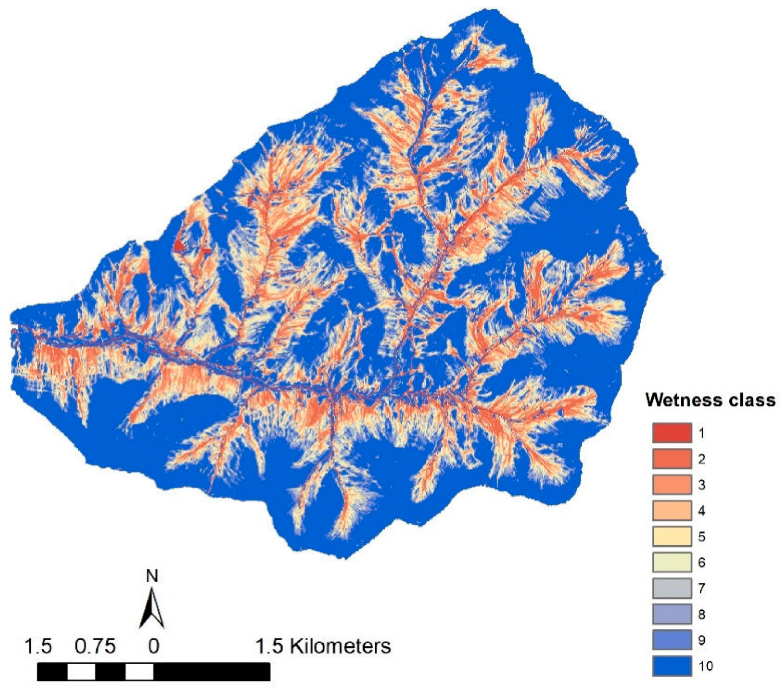
In SWAT-with-impervious-layer (SWAT-wil), the hydrological response is based mainly on the landscape position, and therefore a landscape position factor needs to be added to each HRU. To do this, we ranked the HRU from the greatest topo-index (wettest) to the lowest (driest) into wetness classes (Figure 1). Note that we assumed that the land use was included indirectly because the landscape position determines crops grown and not the opposite [28]. For example, in soils with a restrictive layer at shallow depths in the humid Catskill Mountains, forests are found on the steep and fast draining hillslopes, agricultural crops on the mid and lower slopes with sufficient water, and grassland or marsh plants in the wet valley bottoms [23]. Additional details of the approach can be found in Reference [17].
2.1. SWAT-2012
The SWAT-2012 model keeps track of soil water content, SW* (mm) at each time step by:
where is the moisture content at the previous time step, Δt = 1 for a daily time step, P* (mm d−1) is the effective rainfall and equal to the precipitation minus both the evapotranspiration and infiltration excess runoff. is the lateral flow per unit area in (mm d−1), is the percolation of soil water from the bottom of the soil profile. The * superscript indicates that the units in SWAT were used and the SWAT2012 superscript indicates that the derivation of the flux was particular to SWAT-2012.
When SW exceeds the saturated soil water content (product of the saturated moisture content, θs, and the soil depth D (mm), the soil profile saturates to the surface and excess soil water becomes saturated overland flow per unit area, (mm d−1):
From Equation (6), soil saturation and saturation excess overland flow are most likely to occur where both percolation and lateral flow are restricted. In SWAT-2012, an impervious layer set at the bottom of the soil profile completely restricts percolation ; in which case combining Equations (6)–(8) reveal that the overland flow is primarily determined by soil saturation and lateral flow.
Lateral flow in SWAT only occurs when the soil is above field capacity. This is facilitated mathematically by introducing a soil water storage parameter, that has a storage of zero when the soil is at field capacity, hence:
where is the moiture content at field capacity.
The lateral flow per unit area (mm d−1) in SWAT-2012 is expressed as [29]:
where a is an adjustment factor that is hardcoded to 1 in the model computer code, 0.024 accounts for unit conversions mm to m and from hour to day; L*SWAT2012 (SLSOIL in SWAT) is the slope length (m) and K*sat is given on an hourly basis in mm h−1; SW*excess is the storage of water above field capacity per unit area in mm and φd is the drainable porosity and is taken as the difference between the soil water contents at saturation and field capacity. Lateral flow, thus, only occurs when the soil is above field capacity. Equation (12) can be rewritten in consistent metric units of length (L) and time (T) without the 0.024 unit conversion factor as:
where CSWAT2012 is the fraction lost in the lateral flow of water stored in the HRU above field capacity. Note that the variables without a star superscript have metric units that are internally consistent and do not have a constant for converting units, but otherwise, Equations (13) and (14) are the same as Equation (12).
2.2. SWAT-wil
In SWAT-wil, the hydrological response is based mainly on the landscape position, and therefore, a landscape position factor needs to be added to each HRU. To do this, we used the topographic wetness index (Figure 1) as an additional variable in defining HRUs (as described in Reference [17]). These HRUs are further grouped into those that have a hardpan and percolation is restricted, and those that have an unrestricted soil profile and percolation to the groundwater. This classification follows that of Savenije [20] with the exception that the hillsides, which are dominated by subsurface flow, will produce surface runoff when the water table reaches the surface during a rainstorm.
The HRUs on the hardpan soils are ranked according to the topographic wetness index (i.e., their landscape position). Runoff amounts are varied by the capacity to store water in the HRUs. The HRUs downhill (with a large topographic wetness index) are kept wetter than the HRUs uphill. During a rainstorm, the wetter HRUs spill over first generating the overland flow. Differences in moisture content between HRUs are achieved by setting the percolation to zero and varying the amount of lateral flow with less lateral flow directed to the outlet for downhill HRUs than for the uphill HRUs (i.e., the lateral flow is negatively correlated with the moisture content).
In SWAT, the spatial variation of lateral flow, and thus, also of saturation overland flow, is largely determined by variation in the slope (sin a), saturated lateral conductivity (K), and the hillslope length (L) in Equations (13) and (14). In the version of SWAT-wil presented here, we take an alternative approach to calculating lateral flow. As described below, we re-derive the lateral flow equation for HRUs with a restrictive layer and utilize a spatial distribution of available storage (Equation (3)) to determine the spatial variation of lateral flow, and thus, of saturated overland flow.
As mentioned above, SWAT-wil separates the watershed in two parts: (1) the hillside with a restrictive layer at shallow depth on which during wet periods a perched water table forms and (2) uplands with deep soils in which the water infiltrates and feeds the regional groundwater. While the assumption of uniform lateral flow and percolation for an HRU independent of landscape position as assumed in SWAT-2012 is reasonable for relatively flatter terrains (e.g., the southern US Plains), in landscapes such as the northeastern USA and the Ethiopian highlands, differences in soil water content between upslope and downslope caused by the lateral flow over the restricted layer are critical for generating saturation excess runoff [23].
The lateral flow equation is re-derived for HRUs with the restrictive layers. We assumed as in Sloan and Moore [29] that hillslope is uniform and has an infinite width. The lateral flow per unit width as used in the SWAT-wil model (L2 T−1) for a hillslope can be calculated with Darcy’s law for slopes over 1–2% where gravity dominates:
where h (L) is the water table height along slope and the superscript wil refers to the parameter use in the SWAT-wil model. In SWAT-2012, a sink term r is already taken into account by updating the water contents before the lateral flow is calculated. Thus r = 0.
The relationship between the perched water table height, h, and the amount of water above field capacity, SWexcess (L3 L−2), can be written when the capillary fringe is neglected as:
where SWexcess (L3 L−2), is the amount of water in the profile above field capacity per unit area and φd (L3 L−3) is drainable porosity and is equal to (θs − θfc), where θs is the saturated water content and θfc is soil water content in the unsaturated zone above the water table. Combining Equations (15) and (16) gives:
As noted in the previous section, the HRUs in SWAT-wil are ranked along the hillside using the topographic index (Equations (4) and (5)) and for each HRU a separate water table (equivalent to SWexcess in SWAT-2012) is determined. These soil water content and corresponding water table height (as will see below) are found using the SCS curve number interpretation expressed in Equation (3) with the considerations below.
In SWAT-2012 (and similarly in SWAT-wil), percolation and lateral flow only occurs when the soil water content of the HRU is above field capacity. By setting the percolation out of the rootzone to zero, the soil water content is only a function of lateral flow and evaporation. The evaporation is equal to the potential rate when the soil is above field capacity. Consequently, the lateral flow is a unique function of the soil water content and determines the amount of water drained laterally from the HRUs along the slope.
To find both the lateral flow and soil water content when the percolation is zero for each time step for each HRU per unit area (hillslope with unit width and unit length) along the hillside in SWAT-wil, , we first divide both sides in Equation (17) by Lwill:
Each term in Equations (18) and (19) is now dependent on the position of the HRU on the hillslope in the watershed. Since there are no other fluxes at the time that the lateral flow is calculated in SWAT, the flux per unit area in Equation (18) can be written based on the conservation of mass equation for each HRU as:
Combining Equations (18)–(20) and integrating with the initial condition that the soil is saturated (such that occurs after a large storm), we find that for the HRU that are saturated:
where SW0 is the saturated soil water content of the rootzone for an HRU. Using the first two terms of the exponential series, Equation (21) can be written as:
From Equation (22), we find that the amount of water lost per unit area over a time Δt is (SW0 Cwill Δt) and is, thus, equal in absolute value to σ in Equation (3), that is defined as the amount of water to saturate the soil for the HRU in the wetness class. Hence:
Combining Equations (3) and (23) gives, for each HRU, the fraction of the water that drains from the HRU:
Thus, by using Cwill expressed in Equation (24) instead of CSWAT2012 (Equation (14)) for each HRU that is located on an impermeable layer in SWAT-2012, we have created SWAT-wil which has a water table that varies along the hillslope as a function of As, where As is the likelihood of the area remaining unsaturated; As is zero for the area always being saturated and 1 for most unlikely to become saturated. For As = 0, Cwill = 0 (Equation (24)) and the area remains near saturation even when it does not rain the next day (Equation (22). Only evapotranspiration will lower the moisture content. The fractions of water lost, CSWAT2012, and thus Cwill cannot be directly input into SWAT. The slope length Lwill is the input variable (Equation (19)) that can be used to determine the fraction lost for each wetness class.
Overland flow is simply the amount of rainfall that is in excess of the water that can be stored in the soil (Equation (11)). Thus, for example, any rain that falls on the area with As = 0 will be overland flow.
3. Materials and Methods
The main intent of this manuscript is to demonstrate that SWAT-wil can simulate saturation excess overland flow and spatially distributed runoff areas. For that reason, we compared the simulation results of SWAT-wil with SWAT-HS (simulating saturation excess runoff) and SWAT-2012 (simulating infiltration excess runoff). In this study we used the same SWAT-HS and SWAT-2012 model set up by Reference [17] for Town Brook watershed in the Catskill Mountains.
3.1. Town Brook Watershed
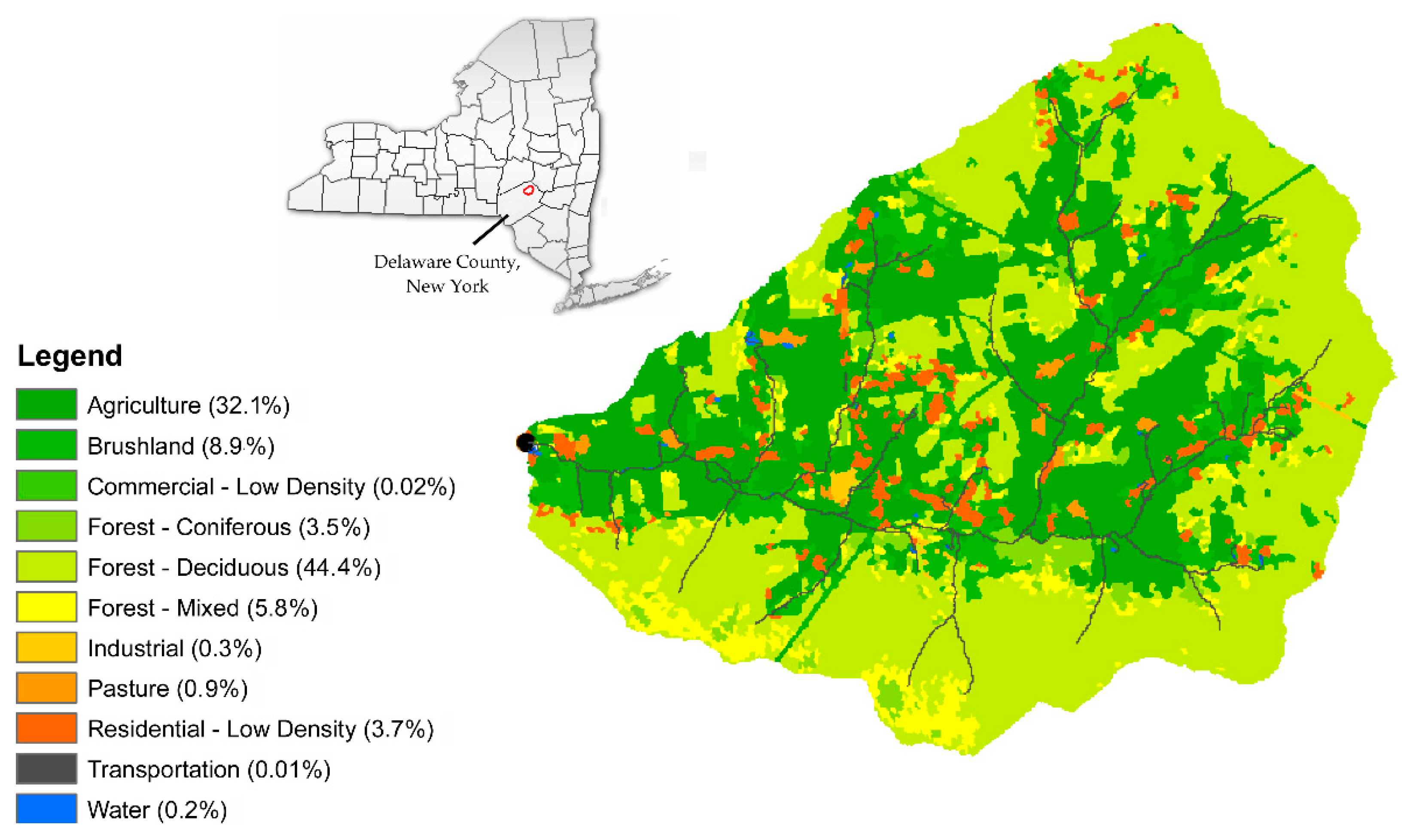
In the 37 km2 Town Brook watershed in the Catskills, NY (Figure 2), the observed extent of saturated areas in 2006 and 2007 were available from previous studies [23,29,30]. The average annual temperature is 8 °C and average annual precipitation is 1123 mm a−1. The landscape is characterized by steep to moderate hillslopes of glacial origin with shallow permeable soils. Elevation ranges from 493 to 989 m. Most soils are silt loam and silty clay loam overlaying a glacial till. The upper terrain on the north facing slope of the watershed is characterized by shallow soil (average thickness 80 cm) overlaying fractured bedrock, steep slopes (average slope 29%), and deciduous and mixed forests (60% of the watershed). The south facing slopes and lowland areas of the watershed have deeper soils (average thickness 180 cm) underlain by a dense fragipan restricting layer, more gentle slopes (average slope 14%), and are predominantly occupied by pasture and row crops (20%) and shrub land (18%). Water and wetland comprise only 2% of the watershed while impervious surface is insignificant. The dominant land cover is forest with 32% agricultural land (Figure 2).
3.2. Description of SWAT-Hillslope
The SWAT-Hillslope model (SWAT-HS) is a modification of the SWAT-2012 model for simulating saturation-excess runoff. Similar to SWAT-wil, HRUs are redefined according the topographic index, but unlike SWAT-wil, it adjusts the basic SWAT code by introducing a surface aquifer in which infiltrating water in excess of soil field capacity is added [17]. This surface aquifer routes lateral flow from “drier” to “wetter” HRUs within a sub-basin. Mathematically, the surface aquifer is a non-linear reservoir that generates the rapid subsurface stormflow when the watershed is above field capacity. Otherwise, the SWAT-wil input are the same for SWAT-2012. The SWAT-HS model was calibrated using outflow at the outlet of Town Brook and the spatial distribution of the saturated areas, providing one optimum set of input parameters. Details are given in Reference [17].
3.3. Model Setup for SWAT-wil
The three models SWAT-HS, SWAT-wil, and SWAT-2012 were applied to the Town Brook watershed using the same meteorological forcing as was used for SWAT-HS by Reference [17]. Daily precipitation and air temperature data to drive the model were from PRISM [17]. Relative humidity was calculated from air temperature time series assuming dew point temperature equaled minimum daily air temperature. Solar radiation was generated by SWAT. Streamflow data for model calibration were from USGS (gauge #01421618) for the period 1998–2012. The model was run with a 3 year startup period. The 2001–2008 period was used for calibration and 2009–2012 for the validation period.
The SWAT-wil model was constructed with spatial information from the SWAT-HS model with one sub-basin, one land use (the dominant land cover forest), one soil type, and 11 HRUs of which 9 HRUs had the same properties as the first nine of the 10 wetness classes in SWAT-HS (Table 1). The basin level parameters are shown in Table 2.
Wetness class 1 and HRU 1 was less than 1% of the area and consisted of wetlands and the streams, and the subsequent 8 HRUs were divided into approximately 6% of the area increments similar the SWAT-HS (Table 1). Wetness class 10 in SWAT-HS was divided in SWAT-wil in HRU 10a and HRU 10b to allow for infiltration excess during very large storms (HRU 10a) and deep percolation to the groundwater (HRU 10b). The percolation out of the first ten HRUs (1–10a), consisting of 85% of watershed area, was zero by setting the depth of the rootzone profile (457 mm) equal to the depth of the impervious layer in soil profile (DEPIMP). The most upland landscape element (HRU 10b) that contributed to groundwater recharge comprised 15% of the watershed (Table 1). The R2ADJ, an HRU parameter that adjusts the retention coefficient of the runoff curve number equation, was set at 100 to turn off curve-number-based infiltration excess overland flow in HRUs 1–9 and 10b (Table 1).
The value of the fraction lost to interflow Cwill cannot be directly inputted into SWAT currently. We can set the value of Cwill by choosing the appropriate hillslope length, Lwil, which is an input parameter. To calculate Lwil, for each HRU, we substitute Equation (24) into Equation (18).
Noting that SW0/φd is equal to the depth of the root zone, reordering Equation (25), Lwil can be found as:
and becomes written in the same units as used in SWAT-2012 (Equations (6)–(12)):
where Lwil is in m, in mm h−1, and S and D in mm. The hill slope length, Lwil, for the various classes was determined with Equation (23) by calibrating the S value with the daily time step Δt = 1.
3.4. Model Calibration
The discharge data from 2001 to 2008 at the outlet of Town Brook were used for calibration. We initially proceeded to calculate S from the curve number (CN) used in the previous application of SWAT to the Town Brook watershed. Easton et al. [16] found a calibrated CN value of 70 for average antecedent moisture condition II (CNII) for Town Brook. Since Equation (21) assumes an initial saturated condition, CNIII (wet antecedent moisture condition III) should be used. The CNIII value for a CNII of 70 is 84, which gives S = 47 mm. For this S value used in Equation (27), the Lwil lengths were an unrealistically low and overestimated lateral flow, underestimated of overland flow, and poorly simulated the hydrograph. We, therefore, calibrated the S parameter. An S value of 5.8 mm was selected based on the separated surface and subsurface flow components from the SWAT-HS simulations of the hydrograph.
3.5. Code Changes
Three minor code changes were made to SWAT 2012 version 622. We corrected a small coding error in the v.622 code (in sat_excess.f) that did not add the precipitation above saturation to surface runoff. In v.622, the R2ADJ parameter that can be used to turn off CN runoff is only input as a basin wide parameter. We added the ability (in readhru.f) to input R2ADJ by HRU in the input file. Both of these changes may have already been implemented in later official versions of the SWAT 2012 code. Finally, we removed in the v.622 code (in percmicro.f) the restriction on the conductivity when the soil was frozen.
4. Results
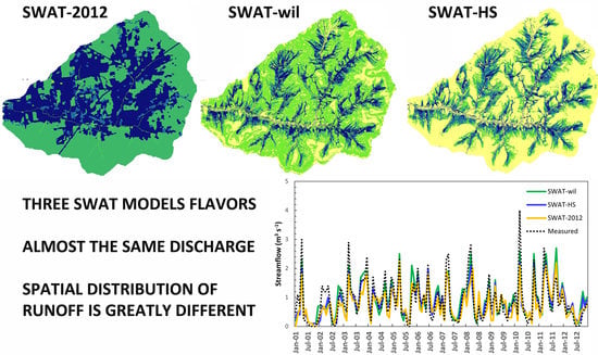
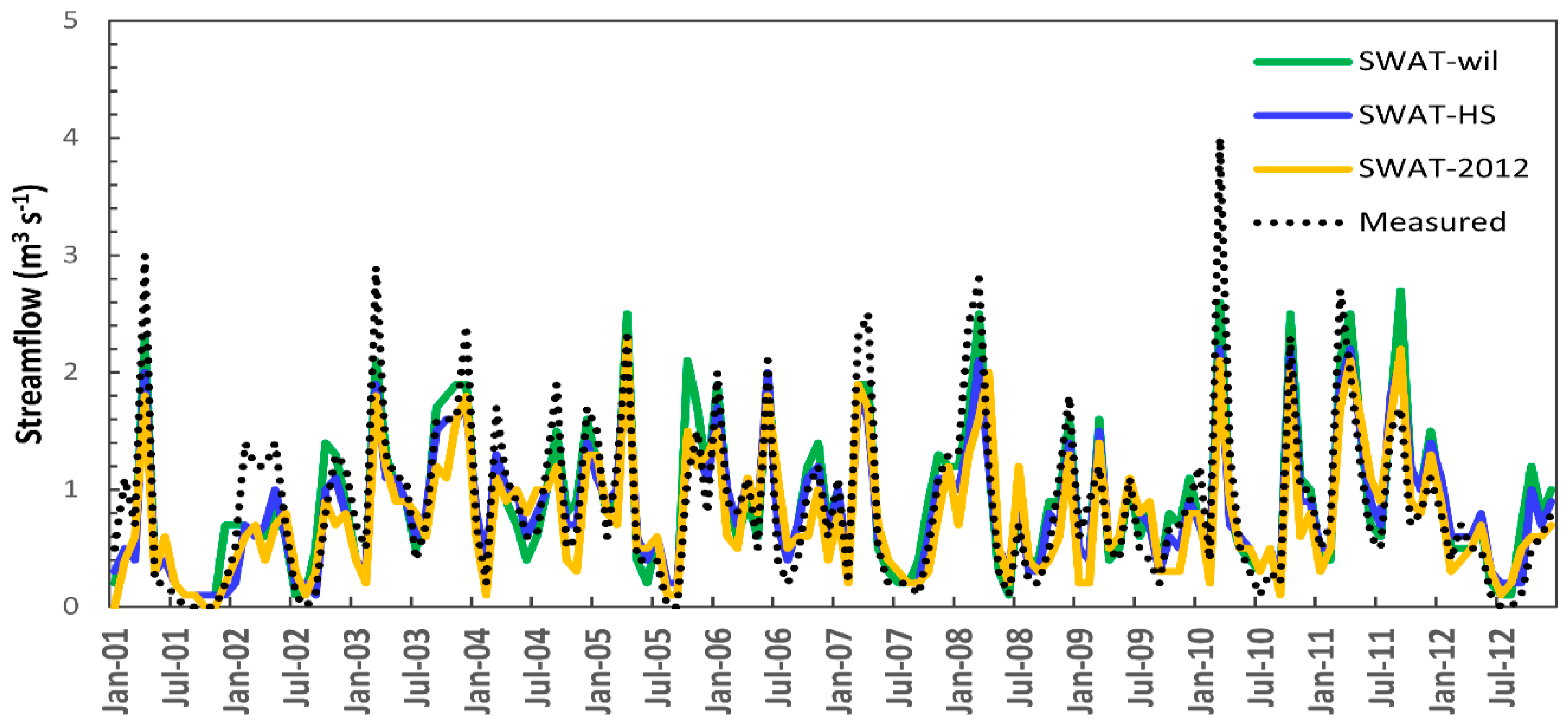
The SWAT-wil model was calibrated for the period 2001–2008 and validated for 2009–2012. The fit of monthly observed and predicted data during the calibration period is shown in Figure 3 and model statistics in Table 3 for both daily and monthly values during calibration and validation. The data indicate that SWAT-wil is capable of simulating the outlet hydrograph for the Town Brook watershed reasonably well. These results are comparable to predictions by SWAT-2012 and SWAT-HS for the same watershed.
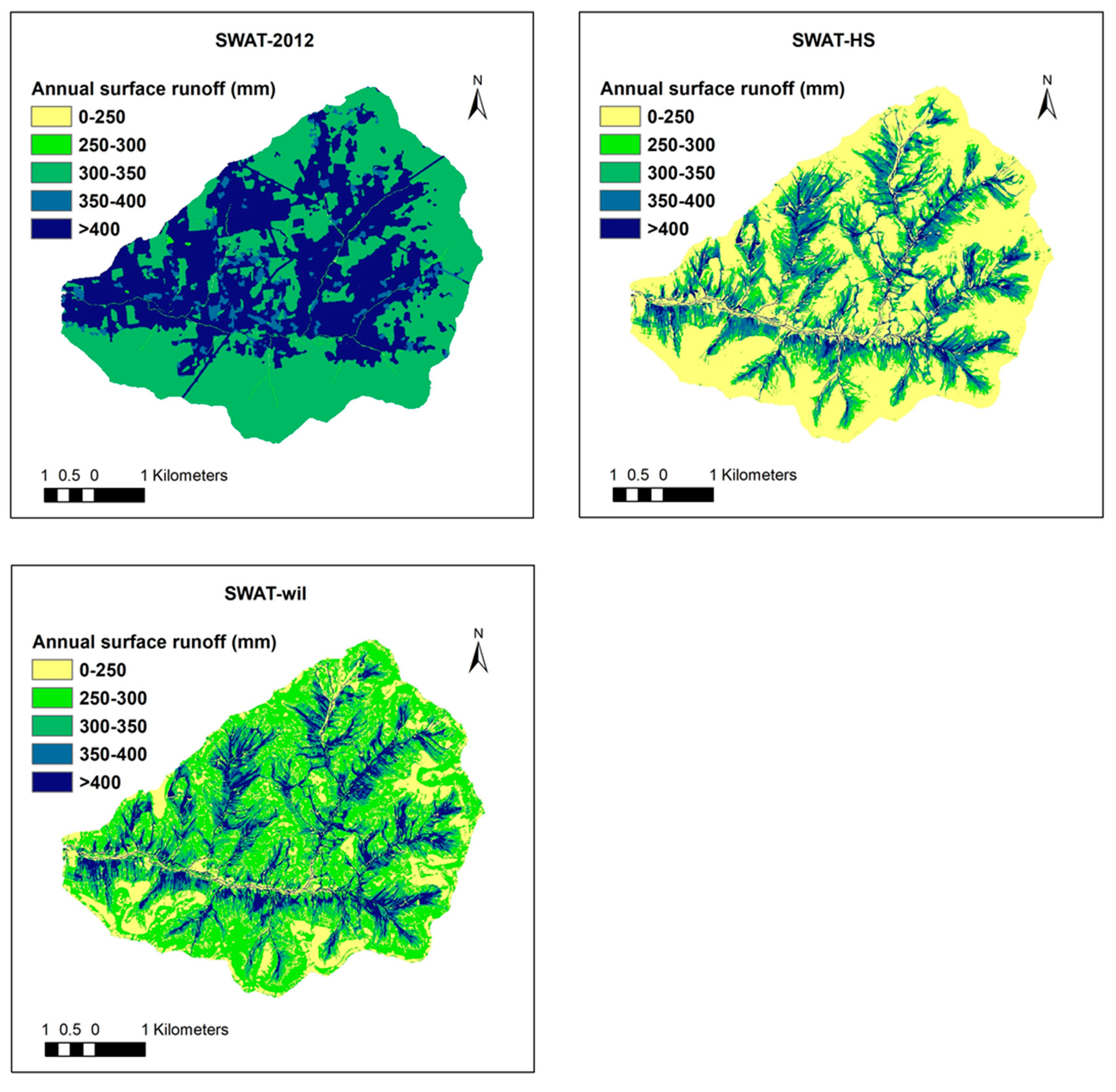
The spatial distribution of surface runoff amounts simulated by SWAT-wil were similar to SWAT-HS (Figure 4). As runoff occurs from the saturated areas, this indicates that the distribution of the saturated areas was similar. Saturated areas were predicted accurately by SWAT-HS [17]. Therefore, the temporal and spatial distribution of surface runoff predicted by SWAT-wil was realistic as well. Overland flow in SWAT-2012 simulated as infiltration excess was much more than either SWAT-HS or SWAT-wil and would imply a much larger area that produces surface runoff (Table 4).
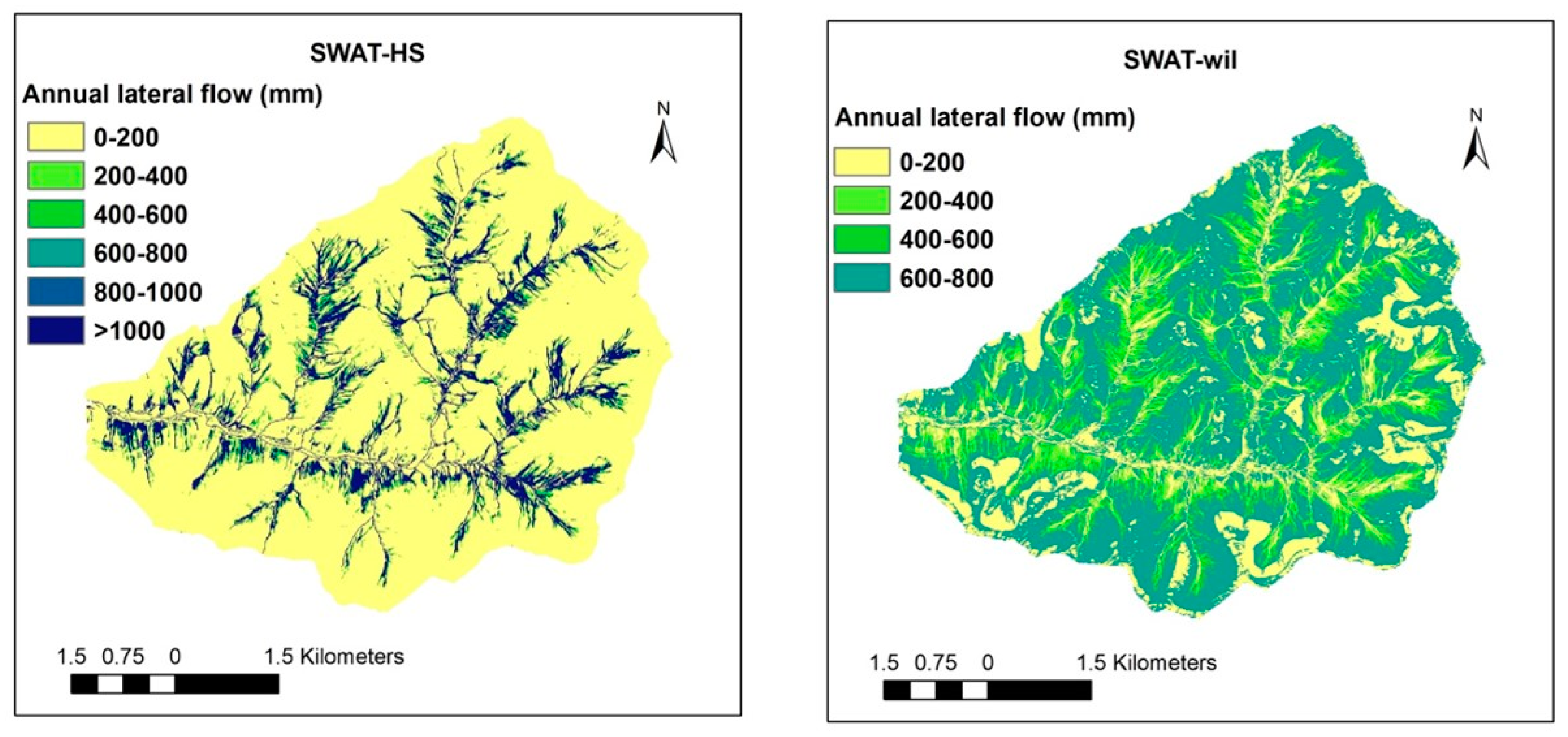
The average simulated overland flow and lateral flow stormflow components of SWAT-wil were comparable to SWAT-HS on an annual basis at the outlet (Table 4). Although the annual amounts were in agreement, the spatial distribution was different (Figure 5). The SWAT-HS model, with its surface aquifer, transports water to the lower HRUs nodes and lateral flow resurfaces as return flow in these areas. In SWAT-HS, 90% of the annual lateral flow exceeding 4000 mm a−1 comes from just 13% of the watershed (HRUs 1,2,3). In SWAT-wil, without a transfer mechanism, 90% of the annual lateral flow comes from 80% of the watershed (HRUs 4–10). The wettest HRUs are, therefore, located downslope and the driest upslope (Figure 6).
Spatial distribution of recharge cannot be validated since the field observations were not available. We assumed in SWAT-wil that the area of groundwater recharge was associated with the smallest topographic index (e.g., HRU10b, Table 1). If the information was available, these areas could be assigned to behave similar to HRU10b and a realistic groundwater recharge distribution could be obtained.
5. Discussion
The northeastern US, just like other humid and sloping areas with restricting layers at shallow soil depth, is dominated by variable source area (VSA) hydrology where runoff and lateral flows occur when the soils are saturated above the restrictive layer [23,31]. In modeling these landscapes with SWAT-wil, the assumption was made that the landscape wets-up similar once the soil moisture is above field capacity despite the complexity of the landscape. This is due to the self-organizing, a principle that underlies all watershed processes [15,16,17,23]. The pattern of saturation depends on the soil depth, slope, and contributing area that define the topographic index. The pattern is independent of vegetation since all plants evaporate at the potential rate when the soil is above field capacity. It is also independent of rainfall intensity because the infiltration rates are greater than the prevailing rainfall intensity.
The concept of hillslope hydrology (and its apparent similarity in wetting up) goes back to Reference [32], inspiring such runoff models as TOPMODEL [27], VIC [33], DHSVM [34], and SMR [35]. Similar to these models, SWAT-HS simulates saturation excess where saturated areas depend on sub-surface lateral inflows from upslope contributing areas. In contrast, soil saturation in SWAT-wil depends only on local rain and snowmelt inputs.
We expected that S values based on variable source interpretation of the CN (Equations (2) and (3)) using realistic values based on past simulations would predict reasonable discharge amounts. This was not the case. We had to calibrate the S value in Equation (24) to match the predicted and observed discharge. As we fitted only the surface and subsurface component of the discharge at the outlet, we were unable to verify the spatial distribution implied by Equation (24) of both the moisture contents and the resulting Cwil values. Other distributions have been employed such as the Pareto distribution in SWAT-HS. Despite this uncertainty, the spatial pattern of VSAs predicted by SWAT-wil and inferred by the Equation (24) with the calibrated S parameter matched the VSA pattern predicted by SWAT-HS (Figure 4).
In Equation (23), the HRU properties are needed to calculate the slope length Lwil. This is counter intuitive because the HRUs are ranked according the topographic index. We can show, however, that Lwil is independent of the HRU physical properties by substituting Equation (4) in Equation (26), the slope length can be directly related to the topographic index, for example:
where R and W are included to make the equation dimensionally correct and are, in practice, set to 1. Thus, the slope length, , for the HRU depends on variables of the topographic index, λ, and the contributing area per unit width, Ac, a measure that the HRU becomes saturated, As, the average water storage in the watershed, S, and the time period of the simulation, Δt. This is not to say that the that is independent of the HRU characteristics, because the topographic index λ calculation (Equations (4) and (5)) includes the physical properties of the HRU (i.e., slope, saturated conductivity, and soil depth).
Not all landscapes have a well-connected macropore network, because in many cases they will be disturbed by roads or other land management practices. The hydrogeomorphic classification of wetlands [36] recognizes such “depression” wetlands with limited subsurface drainage as one of the common wetland types. Thus, saturated areas in a catchment are either dependent on groundwater/interflow inputs or only on local rain and snowmelt inputs as subsurface impoundment. More research is needed as to whether SWAT-wil will apply to either or to some combination of these potentially saturated areas.
In summary, SWAT-will can be used in other application where SWAT-2012 is used because the computer code is not altered. The only differences are that that in SWAT-wil, the HRUs are ranked according to the topographic index and need to have this additional property in order to calculate the Lwil values. The same calibration routines (such as SWAT-CUP) can be used for SWAT-wil with HRUs located on soils with a hardpan.
6. Conclusions
The SWAT-2012 model can be transposed to the SWAT-wil (SWAT with impermeable layer) model that can simulate saturation overland flow and variable source area (VSA) hydrology. This is accomplished by ranking the hydrologic response units (HRUs) with a hardpan according the topographic index and by (1) controlling the lateral drainage by redefining the slope length according to saturation excess interpretation of the SCS curve number; (2) setting the vertical drainage to zero by making the impervious layer at the bottom of the soil profile equal to the root depth vertical; and (3) turning off the SCS curve number generated runoff. The HRUs are treated by SWAT-wil as local sub-surface impoundments that fill up and spill over producing saturated excess overland flow, which depends on hillslope position and local rain and snowmelt inputs to generate saturation overland flow, in contrast to SWAT-HS and other statistical–dynamical runoff models that depend on sub-surface lateral inflows from upslope contributing areas to saturate soils. The SWAT-HS model is a version of SWAT for sloping soils with a hardpan using a statistical–dynamical approach similar to TOPMODEL. The HRUs in SWAT-wil are ranked according to the topographic index.
Predicted spatial distributed runoff areas of SWAT-wil compared favorably with the SWAT-HS (Figure 4) and the simulated discharges for the three models (SWAT-wil, SWAT-HS, and SWAT-2012) were very similar (Figure 3). Thus, the approach presented here provides a method that current users of SWAT-2012 can utilize on catchments with slopes generally over 2% and restrictive layers at shallow depth where variable source area hydrology predominates, and runoff is generated as saturated excess overland flow. Since changes in the code are not required, SWAT-wil can be used for all SWAT applications including SWAT+. The only difference is that in addition to the other physical properties, the HRUs are characterized by the topographic index. In closing, SWAT-wil should provide a more comprehensive process-based framework for simulating VSAs and hydrologic controls on saturated areas.
Author Contributions
The contributions of the authors were as follows: conceptualization, E.M.S. and T.S.S.; methodology, L.H., R.M., M.M., E.M.S., and T.S.S.; software, E.M.S. and L.H.; validation, T.S.S. and R.M.; writing—original draft preparation, E.M.S. and T.S.S.; writing—review and editing, T.S.S., R.M., M.M., and E.M.O.; supervision and project administration E.M.O.
Funding
The work was performed in part with funding of the New York City Department of Environmental Protection (NYCDEP) through subcontracts with CUNY’s Hunter college and Cornell University to provide support for NYCDEP’s Water Quality Modeling program.
Acknowledgments
The impetus of this study was when Fasikaw Zimale (currently at the University of Bahir Dar) relayed to us the suggestion of Raghavan Srinivasan (Texas A & M) that depth to impervious soil layer in SWAT could be used to simulate saturated excess overland flow. This manuscript shows that they were right, but it took many evenings and weekends over a two-year period before a satisfactorily solution could be obtained.
Conflicts of Interest
The authors declare no conflict of interest with respect to changes suggested in the calculation of the parameters in the SWAT model. The funders did not influence the design of the study, the interpretation of data and in the writing of the manuscript.
References
- Arnold, J.G.; Srinivasan, R.; Muttiah, R.S.; Williams, J.R. Large area hydrological modelling and assessment Part I: Model development. J. Am. Water Works Assn. 1998, 34, 73–89. [Google Scholar] [CrossRef]
- Bieger, K.; Arnold, J.G.; Rathjens, H.; White, M.J.; Bosch, D.D.; Allen, P.M.; Volk, M.; Srinivasan, R. Introduction to SWAT+, a completely restructured version of the soil and water assessment tool. J. Am. Water Resour. Assoc. 2017, 53, 115–130. [Google Scholar] [CrossRef]
- Walega, A.; Salata, T. Influence of land cover data sources on estimation of direct runoff according to SCS-CN and modified SME methods. Catena 2019, 172, 232–242. [Google Scholar] [CrossRef]
- Merwin, I.A.; Stiles, W.C.; van Es, H.M. Orchard Groundcover Management Impacts on Soil Physical Properties. J. Am. Soc. Hortic. Sci. 1994, 119, 216–222. [Google Scholar] [CrossRef] [Green Version]
- Tilahun, S.A.; Mukundan, R.; Demisse, B.A.; Engda, T.A.; Guzman, C.D.; Tarakegn, B.C.; Easton, Z.M.; Collick, A.S.; Zegeye, A.D.; Schneiderman, E.M. A saturation excess erosion model. T ASABE 2013, 56, 681–695. [Google Scholar] [CrossRef]
- Brooks, E.S.; Boll, J.; McDaniel, P.A. A hillslope-scale experiment to measure lateral saturated hydraulic conductivity. Water Resour. Res. 2004, 40, W04208. [Google Scholar] [CrossRef]
- Rittenburg, R.A.; Squires, A.L.; Boll, J.; Brooks, E.S.; Easton, Z.M.; Steenhuis, T.S. Agricultural BMP Effectiveness and Dominant Hydrological Flow Paths: Concepts and a Review. J. Am. Water Resour. Assoc. 2015, 51, 305–329. [Google Scholar] [CrossRef]
- Hewlett, J.D.; Hibbert, A.R. Factors affecting the response of small watersheds to precipitation in humid areas. In Forest Hydrology; Pergamon Press: New York, NY, USA, 1967. [Google Scholar] [CrossRef]
- Kane, D.L. Snowmelt infiltration into seasonally frozen soils. Cold Regions Sci. Tech. 1980, 3, 153–161. [Google Scholar] [CrossRef]
- Stähli, M.; Jansson, P.-E.; Lundin, L.-C. Soil moisture redistribution and infiltration in frozen sandy soils. Water Resour. Res. 1999, 35, 95–103. [Google Scholar] [CrossRef]
- Al-Houri, Z.; Barber, M.; Yonge, D.; Ullman, J.; Beutel, M. Impacts of frozen soils on the performance of infiltration treatment facilities. Cold Regions Sci. Tech. 2009, 59, 51–57. [Google Scholar] [CrossRef]
- Moges, M.A.; Schmitter, P.; Tilahun, S.A.; Langan, S.; Dagnew, D.C.; Akale, A.T.; Steenhuis, T.S. Suitability of Watershed Models to Predict Distributed Hydrologic Response in the Awramba Watershed in Lake Tana Basin. Land Degrad. Dev. 2017, 28, 1386–1397. [Google Scholar] [CrossRef]
- Bosch, D.; Arnold, J.; Volk, M.; Allen, P. Simulation of a low-gradient coastal plain watershed using the SWAT landscape model. T ASABE 2010, 53, 1445–1456. [Google Scholar] [CrossRef]
- Arnold, J.; Allen, P.; Volk, M.; Williams, J.; Bosch, D. Assessment of different representations of spatial variability on SWAT model performance. T ASABE 2010, 53, 1433–1443. [Google Scholar] [CrossRef]
- White, E.D.; Easton, Z.M.; Fuka, D.R.; Collick, A.S.; Adgo, E.; McCartney, M.; Awulachew, S.B.; Selassie, Y.G.; Steenhuis, T.S. Development and application of a physically based landscape water balance in the SWAT model. Hydrol. Process. 2011, 25, 915–925. [Google Scholar] [CrossRef]
- Easton, Z.M.; Fuka, D.R.; Walter, M.T.; Cowan, D.M.; Schneiderman, E.M.; Steenhuis, T.S. Re-conceptualizing the soil and water assessment tool (SWAT) model to predict runoff from variable source areas. J. Hydrol. 2008, 348, 279–291. [Google Scholar] [CrossRef]
- Hoang, L.; Schneiderman, E.M.; Moore, K.E.; Mukundan, R.; Owens, E.M.; Steenhuis, T.S. Predicting saturation-excess runoff distribution with a lumped hillslope model: SWAT-HS. Hydrol. Process. 2017, 31, 2226–2243. [Google Scholar] [CrossRef]
- Winter, T.C. The Concept of Hydrologic Landscapes. J. Am. Water Resour. Assoc. 2001, 37, 335–349. [Google Scholar] [CrossRef]
- McDonnell, J.J.; Sivapalan, M.; Vaché, K.; Dunn, S.; Grant, G.; Haggerty, R.; Hinz, C.; Hooper, R.; Kirchner, J.; Roderick, M.L.; et al. Moving beyond heterogeneity and process complexity: A new vision for watershed hydrology. Water Resour. Res. 2007, 43. [Google Scholar] [CrossRef] [Green Version]
- Savenije, H.H.G. HESS Opinions “Topography driven conceptual modelling (FLEX-Topo)”. Hydrol. Earth Syst. Sci. 2010, 14, 2681–2692. [Google Scholar] [CrossRef]
- Steenhuis, T.S.; Collick, A.S.; Easton, Z.M.; Leggesse, E.S.; Bayabil, H.K.; White, E.D.; Awulachew, S.B.; Adgo, E.; Ahmed, A.A. Predicting discharge and sediment for the Abay (Blue Nile) with a simple model. Hydrol. Process. 2009, 23, 3728–3737. [Google Scholar] [CrossRef]
- Steenhuis, T.S.; Winchell, M.; Rossing, J.; Zollweg, J.A.; Walter, M.F. SCS runoff equation revisited for variable-source runoff areas. J. Irrigat. Drain. Eng. 1995, 121, 234–238. [Google Scholar] [CrossRef]
- Schneiderman, E.M.; Steenhuis, T.S.; Thongs, D.J.; Easton, Z.M.; Zion, M.S.; Neal, A.L.; Mendoza, G.F.; Todd Walter, M. Incorporating variable source area hydrology into a curve-number-based watershed model. Hydrol. Process. 2007, 21, 3420–3430. [Google Scholar] [CrossRef]
- Frankenberger, J.R.; Brooks, E.S.; Walter, M.T.; Walter, M.F.; Steenhuis, T.S. A GIS-based variable source area hydrology model. Hydrol. Process. 1999, 13, 805–822. [Google Scholar] [CrossRef]
- Western, A.W.; Zhou, S.-L.; Grayson, R.B.; McMahon, T.A.; Blöschl, G.; Wilson, D.J. Spatial correlation of soil moisture in small catchments and its relationship to dominant spatial hydrological processes. J. Hydrol. 2004, 286, 113–134. [Google Scholar] [CrossRef]
- Beven, K. Rainfall Runoff Modeling: The Primer; John Wiley & Sons, Ltd.: Chichester, London, UK, 2001; p. 360. [Google Scholar] [CrossRef]
- Beven, K.J.; Kirkby, M.J. A physically based, variable contributing area model of basin hydrology/Un modèle à base physique de zone d’appel variable de l’hydrologie du bassin versant. Hydrol. Sci. J. 1979, 24, 43–69. [Google Scholar] [CrossRef]
- Bayabil, H.K.; Tilahun, S.A.; Collick, A.S.; Yitaferu, B.; Steenhuis, T.S. Are runoff processes ecologically or topographically driven in the (sub) humid Ethiopian highlands? The case of the Maybar watershed. Ecohydrology 2010, 3, 457–466. [Google Scholar] [CrossRef] [Green Version]
- Dahlke, H.E.; Easton, Z.M.; Lyon, S.W.; Todd Walter, M.; Destouni, G.; Steenhuis, T.S. Dissecting the variable source area concept—Subsurface flow pathways and water mixing processes in a hillslope. J. Hydrol. 2012, 420–421, 125–141. [Google Scholar] [CrossRef]
- Harpold, A.A.; Lyon, S.W.; Troch, P.A.; Steenhuis, T.S. The hydrological effects of lateral preferential flow paths in a glaciated watershed in the northeastern USA. Vadose Zone J. 2010, 9, 397–414. [Google Scholar] [CrossRef]
- Zimale, F.A.; Tilahun, S.A.; Tebebu, T.Y.; Guzman, C.D.; Hoang, L.; Schneiderman, E.M.; Langendoen, E.J.; Steenhuis, T.S. Improving watershed management practices in humid regions. Hydrol. Process. 2017, 31, 3294–3301. [Google Scholar] [CrossRef]
- Hewlett, J.D.; Nutter, W.L. The Varying Source Area of Streamflow. In Proceedings of the symposium on interdisciplinary aspects of watershed management 1970, Bozeman, MT, USA, 3–6 August 1970. [Google Scholar]
- Liang, X.; Lettenmaier, D.P.; Wood, E.F.; Burges, S.J. A simple hydrologically based model of land surface water and energy fluxes for general circulation models. J. Geophys. Res. Atmos. 1994, 99, 14415–14428. [Google Scholar] [CrossRef]
- Wigmosta, M.S.; Lettenmaier, D.P. A comparison of simplified methods for routing topographically driven subsurface flow. Water Resour. Res. 1999, 35, 255–264. [Google Scholar] [CrossRef]
- Mehta, V.K.; Walter, M.T.; Brooks, E.S.; Steenhuis, T.S.; Walter, M.F.; Johnson, M.; Boll, J.; Thongs, D. Application of SMR to Modeling Watersheds in the Catskill Mountains. Environ. Model. Assess. 2004, 9, 77–89. [Google Scholar] [CrossRef]
- Brinson, M.M. A Hydrogeomorphic Classification for Wetlands; Technical Report WRP-DE-4; US Army Corps of Engineers Waterways Experiment Station: Vicksburg, MS, USA, 1993. [Google Scholar]
Figure 1.
Town Brook watershed: wetness classes based on the topographic wetness index.

Figure 2.
Location of the Town Brook watershed and its land use.

Figure 3.
Comparison of monthly time series of streamflow simulated by SWAT-2012, SWAT-wil, and SWAT-HS with measured streamflow in Town Brook for the calibration and validation period 2001–2012.
Figure 3.
Comparison of monthly time series of streamflow simulated by SWAT-2012, SWAT-wil, and SWAT-HS with measured streamflow in Town Brook for the calibration and validation period 2001–2012.

Figure 4.
Simulated surface runoff contributing areas (VSAs) as indicated by average surface flows over 250 mm a−1 component by SWAT-2012, SWAT-wil, and SWAT-HS for the Town Brook watershed.
Figure 4.
Simulated surface runoff contributing areas (VSAs) as indicated by average surface flows over 250 mm a−1 component by SWAT-2012, SWAT-wil, and SWAT-HS for the Town Brook watershed.

Figure 5.
Simulated lateral flow by SWAT-wil and SWAT-HS for the Town Brook watershed. The lateral flows by SWAT-2012 are small and not shown.
Figure 5.
Simulated lateral flow by SWAT-wil and SWAT-HS for the Town Brook watershed. The lateral flows by SWAT-2012 are small and not shown.

Figure 6.
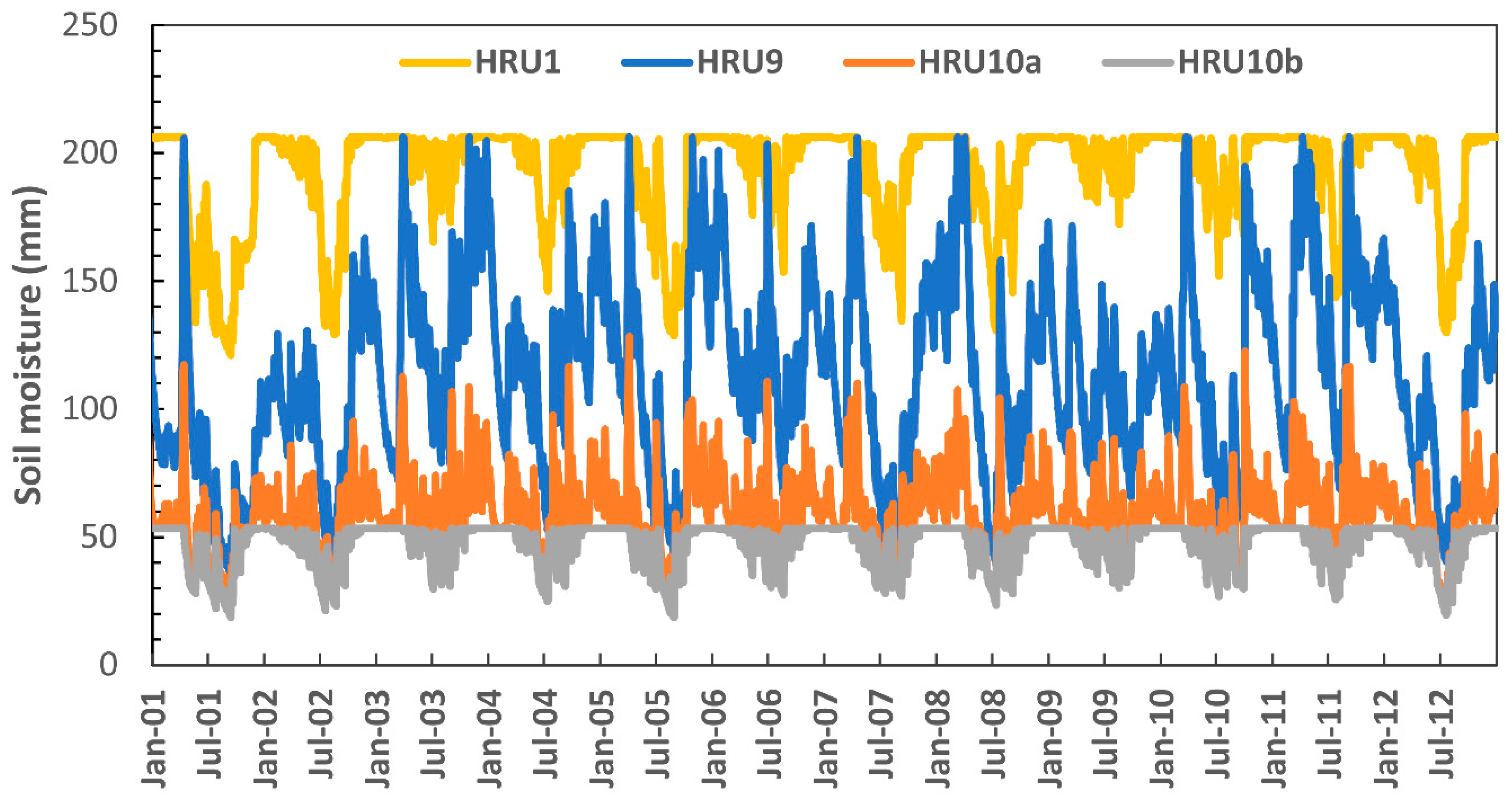
Soil water content of HRUs 1, 9, 10a, and 10b.


Table 1.
Hydrologic response unit (HRU) level parameters for the SWAT-wil model application in Town Brook. DEPIMP is the depth of the impermeable layer, D; KSAT is the saturated conductivity, Ks; HRUSLP is the slope; SLSOIL is the calculated slope length Lwil. R2ADJ a parameter that adjust the SCS curve number runoff. A value of 100 turns the curve number runoff to zero.
| HRU | Topographic Index λ | AreaHRU % | DEPIMP mm | KSAT mm h−1 | HRUSLP mm mm−1 | SLSOIL m | CN2 | R2ADJ |
|---|---|---|---|---|---|---|---|---|
| 1 | >17.7 | 0.59 | 457 | 33 | 0.040 | 1662 | - | 100 |
| 2 | 16.7–17.7 | 6.06 | 457 | 33 | 0.093 | 307 | - | 100 |
| 3 | 15.8–16.7 | 6.24 | 457 | 33 | 0.116 | 135 | - | 100 |
| 4 | 14.8–15.8 | 6.18 | 457 | 33 | 0.128 | 87 | - | 100 |
| 5 | 13.8–14.8 | 6.37 | 457 | 33 | 0.141 | 65 | - | 100 |
| 6 | 12.9–13.8 | 6.20 | 457 | 33 | 0.152 | 51 | - | 100 |
| 7 | 11.9–12.9 | 6.90 | 457 | 33 | 0.167 | 43 | - | 100 |
| 8 | 10.9–11.9 | 6.67 | 457 | 33 | 0.183 | 36 | - | 100 |
| 9 | 10.0–10.9 | 6.04 | 457 | 33 | 0.198 | 31 | - | 100 |
| 10a | 10–7.6 | 33.7 | 457 | 33 | 0.263 | 21 | 35 | 1 |
| 10b | <7.6 | 15 | 6000 | 33 | 0.116 | 1600 | - | 100 |
Table 2.
Basin level parameters for SWAT-wil and SWAT-HS model applications for Town Brook; n.a. is not applicable because the lateral flow was calculated in the SWAT-HS model.
Table 2.
Basin level parameters for SWAT-wil and SWAT-HS model applications for Town Brook; n.a. is not applicable because the lateral flow was calculated in the SWAT-HS model.
| Hydrologic Component | Parameter | SWAT-wil Value | SWAT-HS Value |
|---|---|---|---|
| Snow | SFTMP | −0.58 | −0.58 |
| SMTMP | 1.10 | 1.10 | |
| SMFMX | 7.62 | 7.62 | |
| SMFMN | 2.68 | 2.68 | |
| TIMP | 0.022 | 0.022 | |
| ET | ESCO | 1.00 | 0.691 |
| EPCO | 0.10 | 0.989 | |
| Overland Flow | SURLAG | 2.20 | 4.00 |
| Groundwater Flow | ALPHA_BF | 0.37 | 0.05 |
| GW_DELAY | 3.45 | 31.00 | |
| Lateral flow | LAT_TTIME | 0.22 | n.a. |
Table 3.
Statistical evaluation of different SWAT models of Town Brook using the Nash Sutcliff Efficiency (NSE) and the linear regression coefficient (R2).
Table 3.
Statistical evaluation of different SWAT models of Town Brook using the Nash Sutcliff Efficiency (NSE) and the linear regression coefficient (R2).
| SWAT-2012 | SWAT-wil | SWAT-HS | |||||
|---|---|---|---|---|---|---|---|
| Time Step | NSE | R2 | NSE | R2 | NSE | R2 | |
| 2001–2008 | Daily | 0.53 | 0.54 | 0.61 | 0.61 | 0.65 | 0.64 |
| 2001–2008 | Monthly | 0.67 | 0.73 | 0.81 | 0.82 | 0.80 | 0.86 |
| 2009–2012 | Daily | 0.50 | 0.50 | 0.51 | 0.52 | 0.53 | 0.54 |
| 2009–2012 | Monthly | 0.68 | 0.68 | 0.73 | 0.74 | 0.73 | 0.74 |
Table 4.
Mean daily discharge and stormflow components for 2001–2012 by different SWAT models.
| Flow Component | SWAT-2012 (mm/day) | SWAT-wil (mm/day) | SWAT-HS (mm/day) |
|---|---|---|---|
| Surface runoff | 1.20 | 0.36 | 0.22 |
| Lateral flow | 0.26 | 1.34 | 1.25 |
| Groundwater flow | 0.29 | 0.30 | 0.29 |
© 2019 by the authors. Licensee MDPI, Basel, Switzerland. This article is an open access article distributed under the terms and conditions of the Creative Commons Attribution (CC BY) license (http://creativecommons.org/licenses/by/4.0/).
Share and Cite
MDPI and ACS Style
Steenhuis, T.S.; Schneiderman, E.M.; Mukundan, R.; Hoang, L.; Moges, M.; Owens, E.M. Revisiting SWAT as a Saturation-Excess Runoff Model. Water 2019, 11, 1427. https://doi.org/10.3390/w11071427
AMA Style
Steenhuis TS, Schneiderman EM, Mukundan R, Hoang L, Moges M, Owens EM. Revisiting SWAT as a Saturation-Excess Runoff Model. Water. 2019; 11(7):1427. https://doi.org/10.3390/w11071427
Chicago/Turabian StyleSteenhuis, Tammo S., Elliot M. Schneiderman, Rajith Mukundan, Linh Hoang, Mamaru Moges, and Emmet M. Owens. 2019. "Revisiting SWAT as a Saturation-Excess Runoff Model" Water 11, no. 7: 1427. https://doi.org/10.3390/w11071427
Note that from the first issue of 2016, this journal uses article numbers instead of page numbers. See further details here.