Study on the Raw Water Allocation and Optimization in Shenzhen City, China

Abstract

In order to allocate the raw water of the complex water supply system in Shenzhen reasonably, this paper studied the complex network relationship of this large-scale urban water supply system, which consists of 46 reservoirs, 67 waterworks, 2 external diversion water sources, 14 pumping stations and 9 gates, and described each component of the system with the concepts of point, line and plane. Using the topological analysis technology and graph theory, a generalized model of the network topological structure of the urban water allocation system was established. On this basis, combined with the water demand prediction and allocation model of waterworks, a water resources allocation model was established, aiming at satisfying the guaranteed rate of the water supply. The decomposition and coordination principle of the large-scale system and the dynamic simulation technology of the supply-demand balance were adopted to solve the model. The forward calculation mode of controlling waterworks and pumps, and the reverse calculation mode of controlling reservoirs and waterworks were designed in solving the model, and a double-layer feedback mechanism was formed, which took the reverse calculation mode as outer feedback and the reservoir water level constraint or pipeline capacity constraint as inner feedback. Through the verification calculation of the case study, it was found that the proposed model can deal well with the raw water allocation of a large-scale complex water supply system, which had an important application value and a practical significance.

1. Introduction

The urban water supply system is the front-end water supply subsystem of the urban water resources system. Consisting of a variety of water sources and a variety of water transmission and distribution projects, it is a complex natural and artificial system that is used to meet the water supply needs of different periods with the development of large cities [1,2]. Raw water refers to the natural water resources that have not been processed in the city. It is the main source of water for the life, production and ecology in the city. The allocation objective of raw water in the water supply system is to realize the rational utilization of water in the consumption areas, so as to promote the sustainable development of the society and economy. According to the literatures from all over the world, it is found that there are few studies on the allocation model of the urban water supply system, and that most of the existing studies are only discussed in the relevant water resources allocation model [3,4]. However, the research on the rational allocation model and method of water resources has, as of now, made considerable progress, and it has been continuously developed and perfected in the rapid development of economy, society and science, and technology, achieving many valuable results [5,6]. These studies provide a lot of scientific methods for the study of the optimal allocation of raw water in the urban water supply system on a mesoscale scale.

Various kinds of research work that take the water resources system analysis as a means and the rational allocation of water resources as a goal originated from the reservoir operation optimization problem that was put forward in the 1940s [7,8]. In the 1950s, the research on water resources system analysis developed rapidly; many related models, methods and theories have emerged, such as rough set, fuzzy theory, credibility theory, amongst others [9,10,11]. After the 1960s, with the introduction of system analysis theory and optimization theory and the development of computer technology, the simulation model and solution technology of water resources systems were rapidly studied and applied [12,13]. The earliest water resources simulation model was designed by the Army Corps of Engineers in 1953 to solve the operation of a reservoir in the Missouri River Basin [14,15]. The water resources development plan of the Rio Co1orado basin completed by Massachusetts Institute of Technology [16] in the 1980s is a successful and influential example. This study applied simulation model technology to study the water allocation and utilization in this basin, and put forward the multi-objective programming theory and mathematical model method of water resources planning. At the end of the 1990s, the Danish Institute of Water Resources and Environment [17] successfully developed the integrated water resources planning and management model, i.e., MIKEBASIN, which is a professional model tool applied to the integrated water resources planning and management of river basins or regions. This model is one of the most advanced simulation models of water resources planning and management at present. In 2002, McKinney et al. [18] put forward the framework of a water resources simulation system based on the GIS system, and successfully carried out the research of water resources allocation in river basins. Zhao et al. [19] constructed a new water resources allocation system analysis model based on the analysis of the complexity of the water resources allocation system and its complex adaptation mechanism.

While the water resource allocation model has become a research hotspot, the model optimization technology has been developed rapidly. In 1987, Willis [20] applied a linear programming method to solve the operation and management of surface water and groundwater consisting of one surface reservoir and four groundwater aquifer units. In 1995, Watkins et al. [21] introduced a framework of a sustainable water resources planning model with risks and uncertainties, and established a representative joint water resources scheduling model. At the end of the 20th century, with the rapid development of science and technology, new optimization technologies, such as dynamic programming [22,23,24], a genetic algorithm [25,26], particle swarm optimization [27,28], etc., were applied in the field of water resources, greatly promoting related research on the optimal allocation of water resources [29]. Lu et al. [30] set up a decomposition and coordination model of a large-scale water resources system in Yiwu City, and put forward a method of selecting the best scheme through a hierarchical simulation. Wang et al. [31] studied the application of a genetic algorithm and simulated annealing in the optimal management of groundwater resources, and established a mixed model of the multi-stage simulation and optimization for groundwater. Teegavarapu et al. [32] proposed a reservoir system operation optimization method based on the simulated annealing method.

In summary, the existing research on the water resources allocation model mostly focuses on water resources simulation models and optimization methods, and the research on the water resources allocation model of the urban water supply system is carried out based on the analysis of the characteristics of the model itself and the comprehensive application of theory and the optimization method. Therefore, how to set up a water resource allocation model that can accurately describe the complex hydraulic connection and structure layout of large cities and accord with the actual water supply system, and how to use the corresponding optimization technology to solve it, will be the focus and difficulty of this research.

As mentioned above, the large-scale urban water supply system is a natural and man-made water resources system, in which the water supply pipelines are crisscrossed, the hydraulic links between reservoirs and waterworks are complex, and the structure of the water source network is huge, belonging to a typical complex large-scale system. Consequently, before modeling and solving, a comprehensive analysis of the structural characteristics of the system is necessary, and we need first to establish a generalized structure for the system through topological analysis technology and graph theory, which can reflect the characteristics of the system and be conducive to modeling and solving.

In the generalization of the water supply system, we should focus on the main interconnected reservoirs, waterworks and related pipelines and pumps. After determining the main objects of the water supply system, we need to sort out and summarize the connection relations among these objects, and then describe the water network relations of the whole city. The relationship among these objects in the water supply system is generalized to the relationship of the corresponding graph structure. These objects and their corresponding relations are further generalized to a directed graph model composed of basic graphic elements, such as points, lines and planes. The specific generalization methods of the related objects are shown in

Table 1. Basic graphic elements and their characteristics of the generalization chart of the water supply system.

Basic Element	Object Type	Realistic Objects and Main Characteristics
Point	External water sources	It is integrated into the water supply system as the virtual reservoir.
	Reservoir	It is the water supply reservoir in the system, and it has the regulation capacity.
	User	Mainly refers to the waterworks, including other water users; it is the demand side of the system.
	Convergence node	Pipeline intersection node, no regulation capacity; inflow and outflow are strictly equal.
Line	General pipeline	Closed pipelines, open channels, etc. They usually have a high water head.
	Pressurized pipeline	Including the pipelines that use a pressurized pumping station. The operation cost and head restriction of the pumping station should be considered in the calculation.
	Artesian pipeline	Low-pressure pipeline, because of the low head; the direction and capacity of flow are affected by the water level on both sides.
Plane	Water supply unit	It is composed of point and line elements in the region divided according to the management region or administrative region. It is the basic unit of dispatching decision-making and supply-demand balance statistics.

.

Through the above generalization, the relationship among the related objects in the water supply network can be transformed into the relationship among points, lines and planes in the graph structure. Among them, the water sources, reservoirs, waterworks, pumping stations and sluice gates correspond to the points in the graph structure, and the pipelines correspond to the lines in the graph structure. In the process of generalization, the upstream and downstream relationship between the reservoirs and the supply relationship between the reservoirs and waterworks should be followed.

There are many water sources in large-scale cities’ raw water systems, and the structure of a water supply network is complex. In addition to the influence of various non-technical factors such as politics, economy, environment, decision preference and random natural factors such as rainfall and runoff, achieving reasonable results by using some existing optimization techniques is very difficult for the water allocation in this kind of raw water system. The main research content of water resources operation in large-scale cities focuses on how to conduct the unified dispatching for different water sources under the present hydraulic engineering structure of the water supply system, and how to formulate the optimal operation schemes to meet the raw water demand of waterworks, considering the complex structure and uneven spatial and temporal distribution of water resources. A large number of case studies showed that the dynamic simulation of the water resources supply-demand balance can comprehensively use advanced technologies, such as a system analysis and computer simulation, to describe the complex internal relations and external boundaries of the water resources system in detail [33,34].

This paper will take the raw water dispatching system of Shenzhen as its research object. Based on a comprehensive analysis of the structural characteristics of this system, we will firstly establish a generalized structure of the water supply system of Shenzhen through topological analysis technology and graph theory. This generalized structure can reflect the characteristics of the system and be conducive to modeling and solving. Then, we will establish the optimal dispatching model of urban water by using the dynamic simulation technology of the water supply-demand balance. Through a systematic analysis and technical research, the water supply system in Shenzhen can be scientifically managed, and the optimal allocation of water resources can be realized, which has great theoretical and practical significance.

2. Methodology

2.1. Analysis and Generalization of Raw Water Allocation System in Shenzhen

There are many objects, such as reservoirs, waterworks, and pumps and gates, in the Shenzhen raw water dispatching system, and the system dimension is high, while the amount of data is large. Before formulating the whole city water supply dispatching scheme, it is necessary to make a related analysis and generalization for the whole city water supply network structure, so as to establish a dynamic model, which cannot only reflect the actual situation of the Shenzhen water supply system network, but can also realize the mathematical abstraction through a generalization.

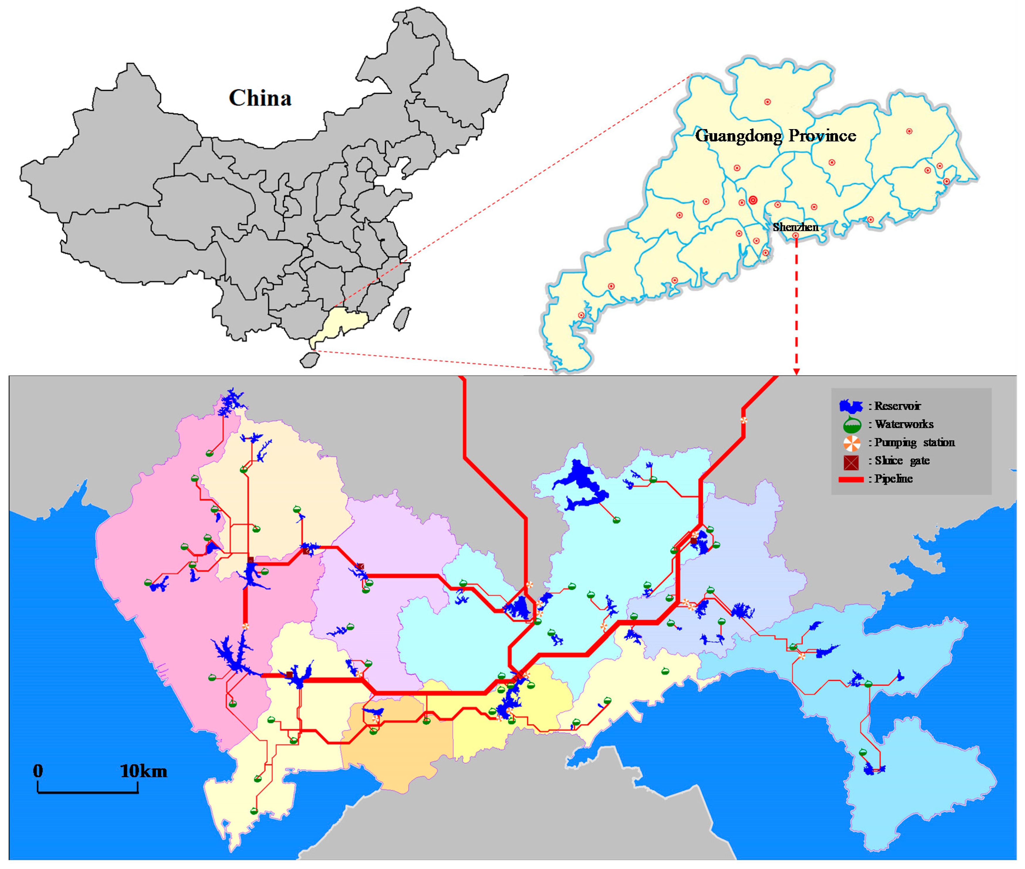
The objects in the actual raw water dispatching system in Shenzhen can be divided into six categories: reservoirs, waterworks, water sources, pumping stations, gates and pipelines. The specific objects in this study include 46 reservoirs, 67 waterworks, 2 external water sources (Dongshen and Dongbu), 14 pumping stations, 9 sluice gates and many connecting pipelines. The main reservoirs, waterworks and their interconnections are shown in Figure 1.

On the one hand, the complexity of the system is manifested in the large number of objects and the large amount of data. On the other hand, it is manifested in the complex relationship among these objects. The water compensation is realized by pipelines between reservoirs, and it has both parallel and series relations. In the water source allocation, the mutual allocation of local water and external water is difficult to consider, but so is the mutual compensation between reservoirs.

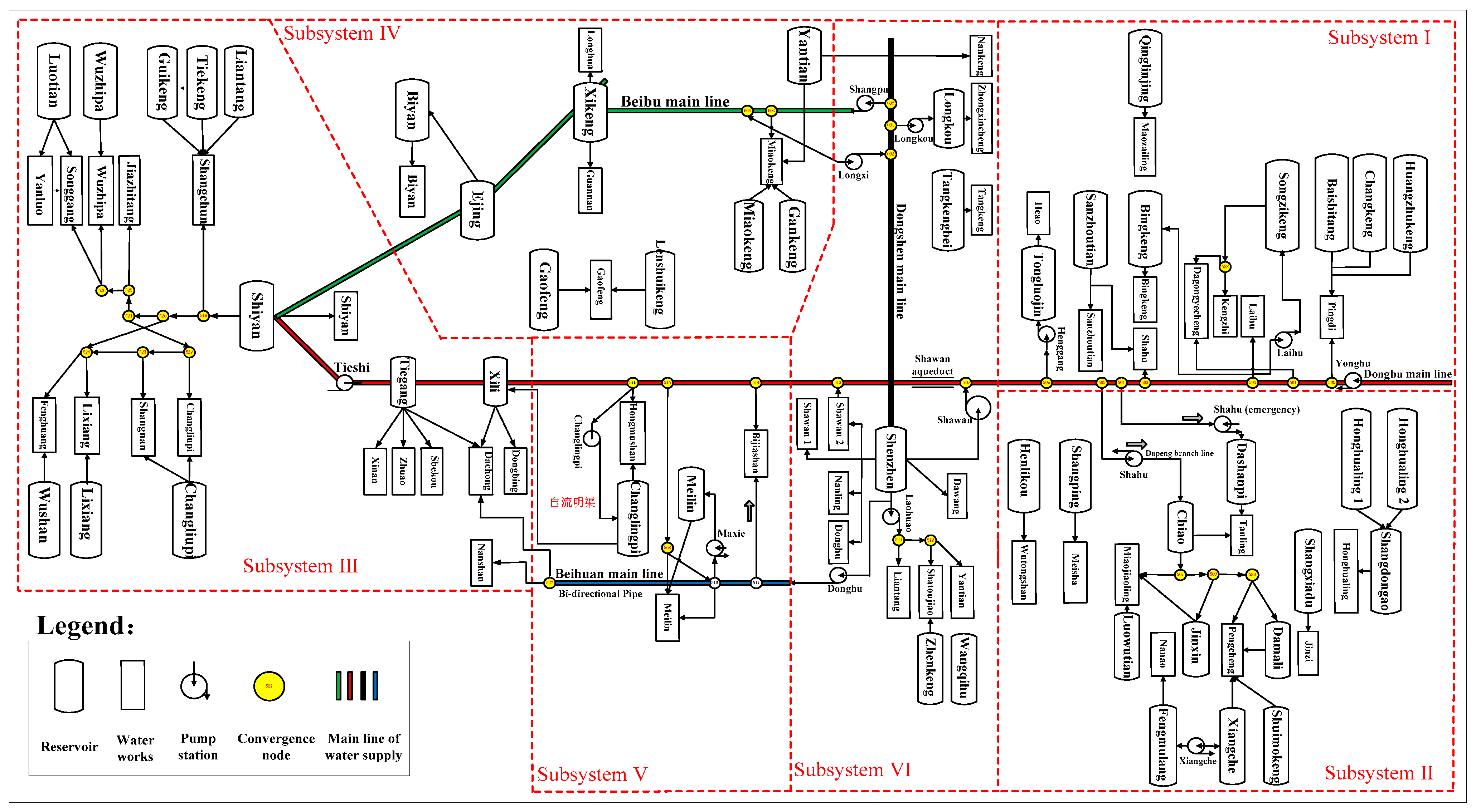
The complex relationship among these objects in the system is the basic starting point of system generalization. Its main relationship can be divided into two categories: the relationship between reservoirs, and the relationship between waterworks and reservoirs. The relationship between reservoirs is mainly manifested in the mutual supply relation of the water volume between interconnected reservoirs, which includes the water supply from upstream reservoirs to downstream reservoirs, as well as the water supply from downstream reservoirs to upstream reservoirs through pumping stations. The amount of water between the two main water supply lines can also mutually supply each other (for example, the water of the Dongshen mainline can be supplied to the Dongbu mainline through the Shawan pumping station). The relationship between reservoirs and waterworks is mainly manifested in the relation of the water intake and supply between reservoirs and waterworks, including the source of water intake, the priority of water intake and the allocation principle of water. Each object in the network is connected by pipelines, which can be divided into two situations: sluice discharge and pumping station lifting. The method of obtaining a pipeline flow is determined by the supply-demand dynamic balance method, except that part of the pipeline needs special treatment. The network structure after the generalization is shown in Figure 2.

2.2. Forecasting Model of Water Demand and Its Allocation in Waterworks

Water source dispatching is based on the prediction of the water demand of waterworks, and its accuracy directly affects the rationality and reliability of dispatching decision-making [35,36]. At present, there are many methods for water demand prediction. A linear regression model, grey prediction model [37], neural network model, support vector machine [38] and other models were applied in urban water demand prediction. As the end-user of the raw water system, satisfying the water demand of waterworks is the basic goal in a water source operation. Therefore, it is necessary to forecast the water demand of the networked waterworks. The forecasting results will be regarded as the boundary condition for formulating water source dispatching schemes, and they are also an important index in the objective function that is used to measure the dissatisfaction depth of waterworks.

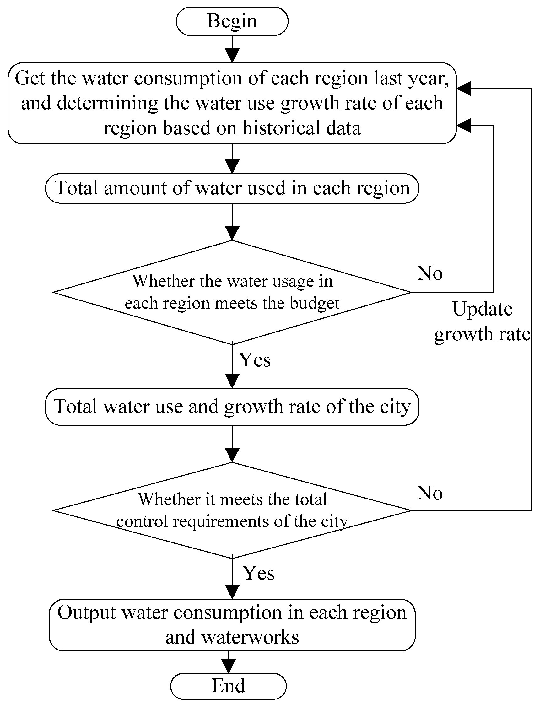
In this paper, through the comprehensive analysis of the historical water consumption data, a suitable mathematical model is constructed by using the combination of the zonal water volume prediction and the single waterworks water volume prediction. The water demand process of each waterworks during the operation period is predicted through this model, and it is taken as the water demand of the system. The idea of the forecasting model is as follows. First, determine the water use growth level of each region, then calculate the water use growth rate and the total water usage of the whole city; after this, coordinate the total water usage of each area according to the plan and control objectives, and control the water use growth rate and total water usage of the whole city, before finally determining the total volume of the water supply of each waterworks and its annual distribution by an iteration calculation.

The formula of water demand forecasting can be expressed as follows:

$$W_t=W_{t,pre}\times R$$

(1)

where W_t is the predicted water demand of a certain region or a certain waterworks in the t-th stage. R is the water consumption growth rate at this stage, and W_t,pre is the corresponding water demand at the same stage of last year.

Because of different economic developments in different regions, the growth rate of the water usage in different regions will be different. Meanwhile, the growth rate of the water supply of different waterworks in the same district is sometimes also different. Therefore, before forecasting the water demand of the whole city, it is important to determine the reasonable water utilization growth rate of each region and the water supply growth rate of each waterworks. The appropriate growth rate can be set according to the different economic development conditions of each area in the forecasting. Generally, at the beginning of the year, the default initial value is set to the growth rate of the water supply of last year relative to the previous year. Then, for the next year, the daily water consumption of each waterworks in each region can be calculated according to the determined growth rate, the total water consumption and annual cumulative value of each region can be calculated, and the total water consumption and growth rate of the whole city can be calculated as well.

In each year’s actual dispatching, through the analysis of the completed dispatching results, the predicted value of the water demand in each region can be revised on a rolling basis, so as to make the annual dispatching results meet the budget of each region as far as possible, while at the same time meeting the requirements of total control for the external water resources in the whole city. This process is not generic; it is mainly based on the water supply situations in Shenzhen City. The water demand forecasting process is shown in Figure 3.

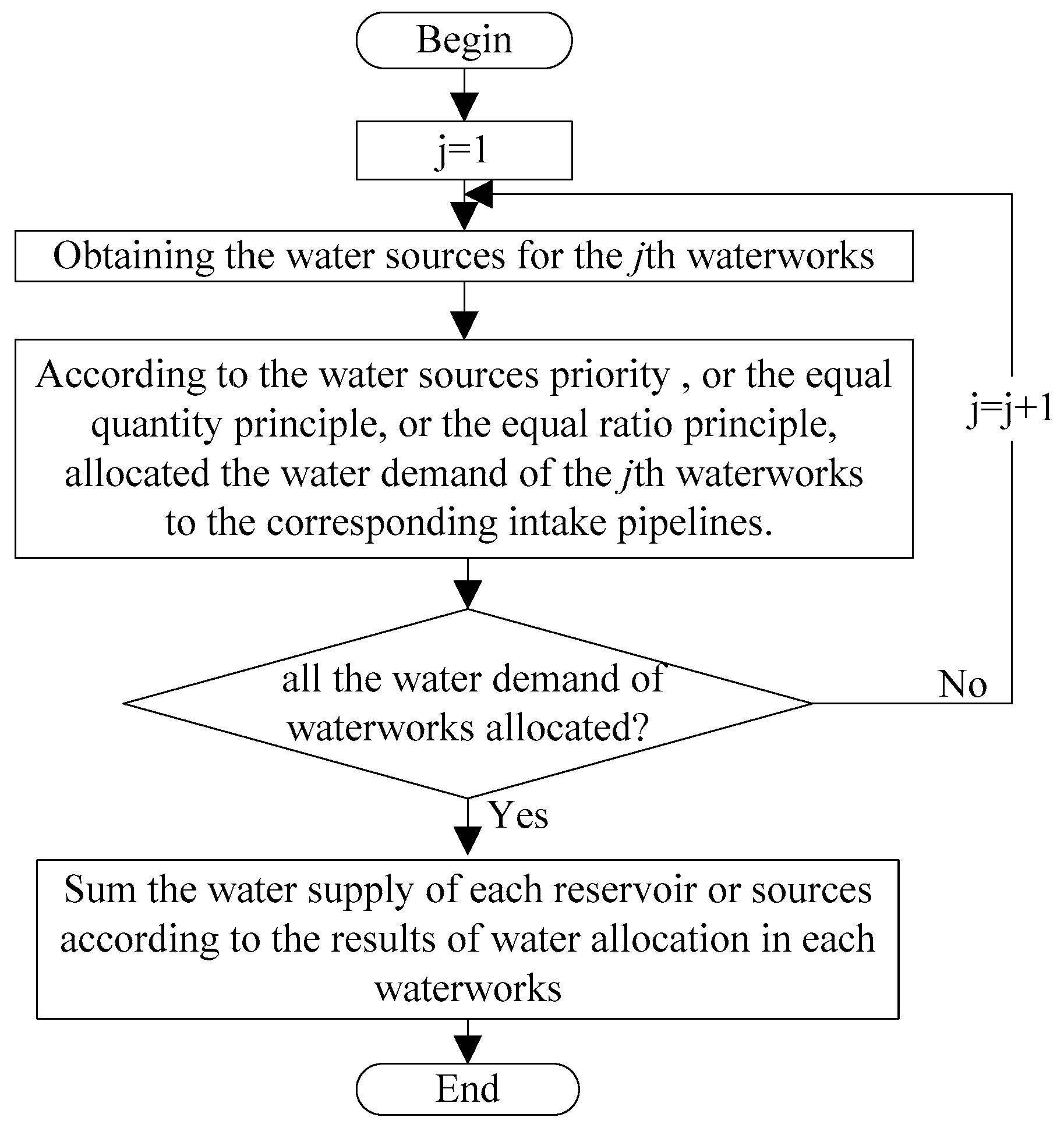
In the process of the water resources allocation, it is necessary to determine the amount of water supplied by reservoirs to waterworks in each stage. The water demand of each waterworks in each stage can be obtained by the forecasting model. However, due to the multi-sources water intake situation of waterworks, the water demand of waterworks in each stage cannot be directly equal to the water supply of reservoirs. The system needs to distribute the water demand of waterworks according to the priority of the water diversion from the reservoir to waterworks, that is, it needs to distribute the water demand of waterworks to each water source. In this paper, three kinds of water allocation methods are designed to deal with this problem: to allocate the water demand according to the priority of diversion of reservoirs, or the principle of equal quantity, or the principle of equal proportion. The flowchart of the water allocation is shown in Figure 4.

2.3. Model of Raw Water Allocation

2.3.1. Objective Function

Because of the status of the Shenzhen Special Economic Zone and the goal of striding towards an international metropolis, the primary task is to ensure the safety of the water supply in meeting the water demand of waterworks or the guaranteed rate of the water supply in Shenzhen. Therefore, considering factors such as the water supply guaranteed rate and the budget balance of each water source management unit, the objective of the raw water allocation model is determined as follows: Maximizing the water supply guaranteed rate of the multi-water source system under the given requirements; the objective function can be expressed as follows:

$$\max P=\max \frac{n\times T-{\displaystyle \sum _{j=1}^n{\displaystyle \sum _{i=1}^T{Time(Q_i)}_j}}}{n\times T}\ge P_0$$

(2)

where the function Time(Q_i)_j is used to calculate the number of times when the water supply of the j-th waterworks is violated. If Q_i < Q_i,plan, then Time(Q_i)_j = 1, and if Q_i > = Q_i,plan, then Time(Q_i)_j = 0.

2.3.2. Constraints

The main constraints of the model include the water balance constraints of the reservoirs [39,40,41], the diversion capacity constraints of the pipelines, the lifting capacity constraints of the pumping stations, the overflow capacity constraints of the gates, the storage capacity constraints of the reservoirs, and so on.

①Water balance constraints of the reservoirs:

$$V_{ji+1}^{}=V_{ji}^{}+W{Y}_{ji}^{}+WZ{C}_{ji}^{}-W{G}_{ji}^{}-WZ{G}_{ji}^{}\begin{array}{cc}& \end{array}j=1,2,\cdots \cdots ,N;i=1,2,\cdots \cdots ,T$$

(3)

②Water balance constraints of the waterworks:

$$G_{ji}^{}=X_{ji}^{}\begin{array}{cc};& G_{ji}^{}={\displaystyle \sum _{k=1}^{M1}W{G}_{ji}^k}\end{array}+{\displaystyle \sum _{k=1}^{M2}W{Y}_{ji}^k\begin{array}{cc}& \end{array}}j=1,2,\cdots \cdots ,m;i=1,2,\cdots \cdots ,T$$

(4)

③Water balance constraints of the water intake nodes (Water source / Virtual reservoir):

$$W{Q}_i={\displaystyle \sum _{s=1}^{S}W{Q}_{si}}={{\displaystyle \sum _{s=1}^S{\displaystyle \sum _{k=1}^{M}W{Y}_{si}^k}}}_{}{{}_{}}_{}{}_{}i=1,2,\cdots \cdots ,T$$

(5)

④Constraints of the capacity of the reservoirs, pumping stations and pipelines:

$$V{M}_{ji}\le V_{ji}\le V{L}_{ji}j=1,2,\dots ,N{;}_{}i=1,2,\dots ,T$$

(6)

$$W{G}_{ji}\le WG{M}_{ji}j=1,2,\dots ,N{;}_{}i=1,2,\dots ,T$$

(7)

$$W{Y}_{ji}\le WS{M}_{ji}j=1,2,\dots ,q{;}_{}i=1,2,\dots ,T$$

(8)

$$W{B}_{ji}\le WB{M}_{ji}j=1,2,\dots ,v{;}_{}i=1,2,\dots ,T$$

(9)

3. Solving of Raw Water Allocation Model

Considering the complexity of the water supply system in Shenzhen, this paper uses the dynamic simulation of the supply-demand balance as the solving method for the water allocation model. In addition, in view of the complex structure, and the large dimension and strong coupling of the model, the decomposition and coordination method of the large-scale system is introduced to solve the model. The water supply system of the whole city is regarded as a complex large-scale system, and the Dongbu and Dongshen mainlines are regarded as two-level coordination subsystems. The objective subsystem is determined by the combination of the management unit and administrative division, and each subsystem is solved separately to alleviate the difficulty caused by the multi-dimension of solving the model. The hierarchical structure of the model is shown in Figure 5. The boundaries of each subsystem are shown by the dotted line frame in Figure 2.

The overall solving steps of the water allocation model can be summarized as follows:

Step1: According to the water demand model, obtain the water demand of each waterworks during the operation period, and determine the initial boundary conditions, including the initial states of the reservoirs, waterworks and pumps.

Step2: Calculate the water allocation step by step according to the hierarchical structure of the large-scale system, and take the water quantity of the first level calculation as the boundary condition of the second level calculation.

Step3: In the second level calculation, first calculate the supply-demand balance of the dispatching schemes formulated by each subsystem, and determine the calculation results of the allocation schemes for each subsystem.

Step4: Then, at a higher level, carry out the coordination and feedback iterative calculation for each sub-problem by means of coordinated variables (diversion water volume), to obtain the overall optimal or satisfactory water allocation scheme for the reservoir subsystem.

Step5: Finally, feedback the optimal solution of the second level calculation to the waterworks, and the waterworks continuously carry out the allocation and feedback according to the results until the water supply guaranteed rate of the waterworks reaches the maximum (the unsatisfactory degree reaches the minimum), and then terminate the calculation.

Step6: Output the optimal water allocation scheme that has the maximum guaranteed rate of the water supply system.

In addition, in view of the complexity and particularity of the Shenzhen water supply system, in the process of solving the above model, a method combining the forward calculation mode and reverse calculation mode is designed to solve the problem. The forward calculation mode controls the waterworks, pump stations and gates, and the reverse calculation mode controls the reservoirs and waterworks. The forward calculation mode refers to the actual operation mode, it is taken as the main method of the system simulation, and it is mainly used to simulate and predict the implementation effect of the operation scheme. As the feedback mode of the forward calculation mode, the reverse calculation mode is mainly used to provide the data reference for the input flow of the pump stations and gates in the forward calculation mode. The comparison between the forward calculation mode and reverse calculation mode is shown in

Table 2. Comparison of the forward calculation mode and reverse calculation mode.

	Control Object	Input	Output	Constraints
Forward calculation mode	Pumping stations, gates, waterworks	Water demand of waterworks, sawtooth flow process of pumping stations, gates	Water shortage of waterworks and terminal state of reservoirs	Capacity constraints of pumping stations, gates and pipelines, and the water level constraints of reservoirs
Reverse calculation mode	Reservoirs and waterworks	Water demand of waterworks, water level requirements of reservoir at the end of the period	Water shortage of waterworks and curve flow process of pumping stations and gates	Capacity constraints of pumping stations, gates and pipelines, and the water level constraints of reservoirs

.

(1) Forward calculation mode

By controlling the flow of the pumping stations and gates, the forward calculation mode uses the water allocation model to simulate the operation process, and calculates the water supply process of the system and the water storage state of each reservoir at the end of the operation period. The calculation process of the forward calculation mode is consistent with the actual operation process. It is the main method for the dispatching and simulation of the system. At the same time, this mode can simulate and predict the implementation effect of the system scheduling schemes under various objectives and show the results. The core calculation process of the forward calculation mode is shown in Figure 6.

In the process of the model calculation, if the results calculated through the initial water demand of the waterworks, and the initial flow process of the pump stations and gates do not meet the requirements, the initial conditions of the waterworks, pump stations and gates need to be reset, and then their control conditions need to be reset according to the calculation results of the reverse calculation mode at this time. Here, the calculated results include the final state of the reservoirs, the water shortage of the waterworks and the discarded water of the reservoirs.

(2) Reverse calculation mode

By setting the expected state of the reservoir, which is generally the water level, the water volume of each reservoir at the end of the dispatching period and the water demand of each waterworks at each stage, this mode uses the water allocation model to simulate the operation process, and calculates the water supply process of the system and the flow process of each pump station and gate. It is another application of the water allocation model under this calculation mode. The results obtained from this reverse calculation mode can provide a basis for setting the control conditions in the forward calculation mode. The core calculation flowchart of this reverse mode is shown in Figure 7.

In the reverse calculation mode of controlling reservoirs and waterworks, aimed at meeting the planned water demand of waterworks and the requirement of the reservoir water level at the end of the operation period, various water sources (external water and self-produced water) in the water supply system are taken as supply resources; and according to the model constraints, the calculation criteria and the dynamic balance principle of supply and demand, the reverse recurrence is carried out from the waterworks at the last level of the network, and the upward catchment calculation is carried out step by step up to the intake port of the water source. If the water level constraints or pipeline capacity constraints are not satisfied in the reverse calculation process, the corresponding constraint boundaries will be used for feedback regulation to reduce the downstream water supply until all the constraints are met. After reducing the downstream water supply, the water demand of the waterworks will certainly be insufficient. The water should be first allocated according to the priority of the waterworks at this time. If the priority is the same, the water demand will be allocated according to the proportion of the water demand of the waterworks. The flow process of the pumping stations and gates calculated by the reverse calculation mode is a curve process with one day as the stage length, which is not conducive to the implementation of the actual operation. Therefore, it is necessary to transform it into a sawtooth flow process and to bring it into the forward calculation mode to check whether the input flow of the pump stations and gates meets the requirements or not.

So far, a double-layer feedback regulation mechanism has been formed, which takes the reverse calculation mode as the outer feedback and the reservoir water level or pipeline capacity as the inner feedback. The solving process of the dynamic simulation of the supply-demand balance based on this double-layer feedback regulation is shown in Figure 8.

4. Case Study

Based on the above water allocation model and the solving method, a case study is carried out in Shenzhen City, which takes the interval of March 2 to March 10, 2013 as the operation period, and takes one day as the length of the operation stage. In this case study, the contexts include the initial boundary setting of the reservoir, waterworks, pump stations and gates, and the water demand calculation of the waterworks and results analysis, etc. In addition, it should be noted that the main object of this study is the raw water and its rational allocation among the waterworks. As for how to deal with such raw water in the waterworks and how to supply water to users after treatment, no relevant research has been done in this case.

4.1. Input Data and Boundary Conditions

The initial boundary conditions of the operation scheme include two parts: (1) the initial state of the reservoirs, waterworks, pump stations and gates, and (2) the water demand of the waterworks during the operation period. The initial state includes the initial state of the reservoirs (including the current water level, current reservoir volume, yesterday’s water supply to the waterworks, etc.), the water demand of the waterworks, and the initial flow of the pump stations and gates at the beginning of the operation period. The initial state of the reservoirs is shown in Appendix

Table A1. Initial state of reservoirs in the whole city on 2 March 2013.

Name of Reservoir	Normal Water Level	Normal Storage Volume	Dead Water Level	Dead Storage Volume	Current Water Level	Current Volume	Yesterday’s Water Supply
Shenzhen	27.12	3348.41	16.56	19.00	27.30	3230.23	114.37
Meilin	58.60	1251.58	30.00	36.25	50.60	775.71	0.00
Xili	29.59	2481.50	18.59	104.00	28.42	2094.20	28.65
Zhengkeng	48.67	38.00	38.20	0.00	45.94	19.14	0.00
Wangjihu	46.07	5.96	39.33	0.00	45.63	0.00	0.00
Shangping	233.20	170.00	219.56	0.00	225.63	53.47	0.00
Tiegang	28.70	9400.00	10.79	60.00	23.01	4198.00	34.46
Shiyan	36.58	1690.00	26.92	60.00	34.87	1148.00	85.92
Lixin	15.70	698.00	8.00	6.00	11.58	296.00	0.00
Wushan	25.65	220.00	19.00	28.00	22.62	91.00	0.00
Changliupi	23.00	512.60	14.50	13.60	21.83	405.30	0.24
Wuzhipa	27.56	125.00	22.98	22.00	25.00	57.50	1.49
Luotian	32.77	2050.00	16.96	50.00	19.25	99.80	1.36
Liantang	16.31	156.00	7.83	1.30	13.93	98.00	0.00
Tiekeng	20.00	299.00	8.07	0.91	13.60	62.20	0.00
Guikeng	18.13	70.00	9.36	1.00	3.50	27.00	0.00
Biyan	41.14	66.00	32.29	1.00	40.01	48.66	0.00
Ejing	55.54	451.00	44.10	53.00	46.18	92.38	0.00
Xikeng	75.41	1900.00	65.00	4.00	70.52	1087.90	39.40
Changlingpi	62.50	1448.00	39.60	15.64	54.79	679.53	0.00
Gaofeng	85.62	294.00	70.23	3.00	74.80	58.80	0.00
Longkou	72.01	924.30	53.00	7.30	62.32	273.22	19.20
Qinglinjing	58.50	1803.00	48.30	31.00	50.00	326.32	4.31
Tangkengbei	71.89	75.00	64.95	4.00	66.70	11.00	0.00
Tongluojing	80.00	1883.00	60.00	257.00	0.00	0.00	0.00
Bingkeng	64.81	300.00	54.36	10.56	57.62	72.83	0.00
Huangzhukeng	56.02	223.00	42.00	13.00	48.50	69.00	0.00
Changkeng	52.20	128.00	42.00	4.30	47.30	50.50	0.00
Baishitang	73.16	97.00	62.60	4.50	68.00	39.50	0.00
Yantian	48.60	968.00	47.05	596.00	0.00	0.00	0.00
Miaokeng	71.99	123.00	58.00	0.00	68.19	52.00	0.00
Gankeng	79.72	260.00	69.67	0.00	75.77	101.00	0.00
Chiao	82.00	1475.00	27.00	25.00	78.55	1093.00	3.56
Dashanpi	57.46	378.10	45.86	3.00	52.47	155.70	0.00
Sanzhoutian	313.11	720.00	301.10	20.00	307.68	282.00	0.36
Honghualing (Up)	182.17	303.50	163.49	5.20	165.93	19.43	0.00
Honghualing (Down)	153.49	212.00	137.60	7.00	150.29	131.80	0.00
Shangdongao	121.39	140.00	97.37	2.00	116.65	97.09	0.00
Shangxiadu	261.90	103.00	245.54	6.00	253.50	42.20	0.00
Songzhikeng	66.00	2450.00	50.00	126.00	59.09	1266.00	13.84
Luowutian	50.57	200.00	44.32	30.00	33.58	157.40	0.00
Jinxin	98.15	732.00	79.87	16.00	93.62	438.00	2.50
Damali	21.70	288.00	12.00	18.00	17.95	167.00	0.93
Shuimokeng	55.05	130.00	36.12	4.00	50.00	76.49	0.00
Xiangche	49.47	1021.00	13.10	19.53	22.00	22.20	0.00
Fengmulang	49.47	440.00	40.76	78.63	45.74	258.77	0.40

. For a comparison, in Appendix Table A1, besides the current water level, the current reservoir volume and yesterday’s water supply to the waterworks, some characteristic values of the reservoir (such as the normal water level, dead water level, and the corresponding storage capacity) are also provided. In addition, the unit of the water level in Appendix Table A1 is the meter, and the unit of the reservoir storage capacity and water volume is 10⁴ cubic meters.

The water demand of waterworks at the beginning of the operation period (March 2, 2013) is shown in Appendix

Table A2. Initial status of waterworks on 2 March 2013.

Areas of Waterworks Located	Name of Waterworks	Water Demand	Accumulated Water Supply in This Year
Former special zone	Donghu	27.2555	1292.01
Former special zone	Bijiashan	18.3357	1050.77
Former special zone	Meilin	37.862	2127.28
Former special zone	Dachong	28.45	1692.79
Former special zone	Nanshan	8.6856	593.74
Former special zone	Shekou	2.83	91.54
Former special zone	Liantang	2.572	119.81
Former special zone	Shatoujiao	1.9942	95.15
Former special zone	Yantian	3.54	204.87
Former special zone	Meisha	0	0
Former special zone	Dawang	0.52	28.65
Baoan district	Xinan	0	0
Baoan district	Zhuao	31.63	1753.94
Baoan district	Shiyan	8.95	482.97
Baoan district	Shiyanhu	0.021	1.39
Baoan district	Lixin	6.41	355.77
Baoan district	Fenghuang	11.36	567.18
Baoan district	Shangnan	5.71	343.51
Baoan district	Changliupi	19.31	1037.18
Baoan district	Wuzhipa	12.91	701.05
Baoan district	Songgang	5.41	277.91
Baoan district	Yanluo	1.3602	89.46
Guangming new district	Jiazhitang	13.32	712.79
Guangming new district	Shangchun	2.41	132.7
Guangming new district	Yulv	1.09	43.49
Guangming new district	Changzhen	0.55	27.9
Guangming new district	Biyan	0	13.2
Longhua New District	Longhua	23.4	1192.9
Longhua New District	Hongmushang	9	587
Longhua New District	Gaofeng	0	0
Longhua New District	Guangnan	16	885.7
Longhua New District	Dalang	3.5	38.6
Longhua New District	Baochang	0.4	9.2
Longhua New District	Damao	0	0
Longgang district	Zhongxincheng	19.2	1167.5
Longgang district	Laihu	9.1633	441.5
Longgang district	Maozailing	4.3146	272.72
Longgang district	Bingkeng	2.0889	125.01
Longgang district	Nankeng	0	108.01
Longgang district	Tangkeng	0	0
Longgang district	Heao	0	0
Longgang district	Miaokeng	0	34.43
Longgang district	Egongling	0	55.7
Longgang district	Pingdi	4.8755	252.79
Longgang district	Shawang one	3.81	182.6
Longgang district	Shawang two	19.6378	1031.54
Longgang district	Nanling	2.52	138.86
Longgang district	Jixia	0.55	27.28
Longgang district	Danzhutou	0.99	55.34
Longgang district	Shatangshi	0.61	17.96
Pingshan New District	Tangling	3.8	203.6
Pingshan New District	Honghualing	0	0
Pingshan New District	Sanzhoutian	0.357	25.94
Pingshan New District	Jingzhi	0	0
Pingshan New District	Shahu	2.4	130.21
Pingshan New District	Kengzhi	4.6248	220.44
Pingshan New District	Dagongyecheng	3.6137	193.55
Dapeng New District	Miaojiaoling	2.5	150.9
Dapeng New District	Pengcheng	1.377	60.1
Dapeng New District	Nanao	0.395	23.42

. The unit of the water demand and cumulative water supply is 10⁴ cubic meters in Appendix Table A2. The initial flow of the pumping stations and gates at the beginning of the operation period (March 2, 2013), and the design maximum flow, are shown in

Table 3. The initial state of the pump stations and gates on March 2, 2013.

Time	Name of Pump Stations and gatEs	Initial Flow (104 m3/d)	Max Flow (104 m3/d)
2 March 2013	Yonghu pump station	189.2	259.2
2 March 2013	Shawan aqueduct (gate)	1403.2	1814.4
2 March 2013	Xitie gate	121.0	2160
2 March 2013	Tieshi pump station	84.43	518.4
2 March 2013	Donghu pump station	60.7	933.12
2 March 2013	Laohuao pump station	8.1	194.4
2 March 2013	Shisong branch line gate	77.0	714.5

. Only the case in which the flow of the pumping stations and gates is over zero is provided in this table, while the other initial flows of the pumping stations and gates are all zero. The unit of flow in Table 3 is 10⁴ cubic meters per day.

Using the water demand forecasting method provided in Section 2.2., the water demand of each waterworks in each stage from March 2 to March 10, 2013 can be obtained, as shown in Appendix

Table A3. Water demand of waterworks from 2 March 2013 to 10 March 2013.

Waterworks	2 March 2013	3 March 2013	4 March 2013	5 March 2013	6 March 2013	7 March 2013	8 March 2013	9 March 2013	10 March 2013	Sum
Donghu	20.46	22.37	0	22.15	0	22.43	21.67	20.34	20.31	149.73
Bijiashan	19.22	18.87	19.7	18.9	20.29	20.76	19.61	19.21	18.88	193.86
Meilin	39.34	41.67	38.61	39.37	41.39	41.66	40.55	38.72	37.37	395.26
Dachong	21.27	23.72	22.88	23.26	23.85	23.94	23.72	22.75	22.58	230.06
Nanshan	14.48	13.33	13.69	10.99	14.31	14.32	13.58	13.04	13.27	134.38
Shekou	4.41	4.46	5.03	4.41	4.54	5.4	3.8	4.25	4.14	45.27
Liantang	2.14	2.27	2.1	2.43	2.49	2.51	2.29	2.16	2.06	22.61
Shatoujiao	2.2	2.2	2.17	2.22	0	2.37	2.52	2.32	2.42	20.6
Yantian	2.24	2.26	2.46	2.18	2.32	2.38	2.28	1.99	2.55	22.63
Meisha	0	0	0	0	0	0	0	0	0	0
Dawang	0.44	0.49	0.49	0.49	0.48	0.5	0.47	0.44	0.42	4.65
Xinan	0	0	0	0	0	0	0	0	0	0
Zhuao	27.31	28.46	28.27	29.04	29.35	30.18	28.33	26.36	26.88	280.41
Shiyan	9.56	10.06	9.59	9.65	9.9	10.19	9.62	9.47	9.17	96.21
Shiyanhu	0.01	0.01	0.01	0.02	0.02	0.01	0.01	0.01	0.01	0.13
Lixin	8.16	8.22	7.54	7.7	8	8.54	7.51	7.82	6.98	76.7
Fenghuang	9.47	10.24	10.46	9.68	10.45	10.08	10.67	9.85	10.28	101.69
Shangnan	5.51	5.21	5.57	5.58	5.19	4.88	6.1	6.32	6.59	57.86
Changliupi	20.23	21.81	19.7	19.54	22.2	23.44	21.19	19.5	18.99	205.09
Wuzhipa	13.48	14.29	13.62	12.83	14.5	15.19	14.6	13.58	13.72	138.98
Songgang	6.06	5.79	5.93	5.94	5.79	5.61	5.71	5.8	5.75	58.01
Yanluo	0	0	0	0	0	0	0	0	0	0
Jiazhitang	12.74	14.1	12.91	12.71	13.07	13.64	13.23	12.17	13.2	130.29
Shangchun	3.04	3.52	3.3	3.16	3.43	3.84	3.54	3.08	3.01	32.82
Yulv	1.09	1.05	1.01	0.99	1.08	1.12	1.12	0.97	0.94	10.39
Changzhen	0.55	0.58	0.56	0.54	0.57	0.58	0.56	0.55	0.54	5.55
Biyan	0	0	0	0	0	0	0	0	0	0
Longhua	21.96	23.76	22.32	22.86	22.77	23.94	22.32	21.78	22.41	224.82
Hongmushang	8.28	8.28	7.36	8.28	8.28	7.36	8.28	8.28	8.28	80.04
Gaofeng	0	0	0	0	0	0	0	0	0	0
Guangnan	14.01	14.79	14.18	14.53	14.01	15.14	14.44	14.01	14.27	142.86
Dalang	0	0	0	0	0	0	0	0	0	0
Baochang	0.47	0.47	0.24	0.12	0.71	0.59	0.71	0.59	0.71	4.96
Damao	0.2	0.2	0.29	0.12	0.08	0.08	0	0	0	0.97
Zhongxincheng	23.25	23.84	22.66	23.25	25.02	24.78	40	22.42	22.77	251.83
Laihu	1	7.01	6.56	6.25	6.49	6.56	6.23	6.26	6.37	58.83
Maozailing	3.79	3.77	3.78	3.79	3.77	3.79	3.78	3.73	3.77	37.72
Bingkeng	0.82	0.83	0.8	0.85	0.84	0.85	0.76	1.11	1.08	9.07
Nankeng	7.43	7.73	7.79	7.19	8.7	8.83	8.66	0	8.44	73.1
Tangkeng	0	0	0	0	0	0	0	0	0	0
Heao	0	0	0	0	0	0	0	0	0	0
Miaokeng	1.25	1.25	1.24	1.17	0.98	1.16	1.3	0	1.28	10.87
Egongling	7.44	8.68	9.42	8.68	9.8	9.18	8.8	8.68	8.68	88.04
Pingdi	4.28	4.41	4.42	4.12	4.47	4.59	4.5	4.08	4.31	43.3
Shawang one	4.72	4.58	5.16	5.27	4.93	5.57	4.72	3.88	3.9	46.59
Shawang two	21.04	21.54	21.28	21.23	21.89	21.58	21.56	20.52	21	198.08
Nanling	2.53	2.68	2.54	2.59	2.75	2.7	2.74	2.38	2.51	25.7
Jixia	0.52	0.55	0.59	0.57	0.59	0.65	0.49	0.43	0.47	5.34
Danzhutou	0.91	1.08	0.97	1.05	1.03	1	1.02	0.84	1	9.71
Shatangshi	0.55	0.54	0.55	0.54	0.56	0.53	0.56	0.54	0.57	5.46
Tangling	2.53	2.58	2.6	2.92	3.28	1.47	1.95	1.53	1.94	21.77
Honghualing	1.66	1.62	1.56	0	1.44	1.61	0.78	1.3	1.45	13.08
Sanzhoutian	0.02	0.03	0.03	0.03	0.03	0.03	0.03	0.03	0.03	0.29
Jingzhi	0	0	0	0	0	0	0	0	0	0
Shahu	0.15	0.1	0.1	0.1	0.1	0.15	0.15	0.15	0.15	1.3
Kengzhi	4.26	4.8	4.39	4	3.27	5.09	6.22	4.35	4.32	44.98
Dagongyecheng	3.23	3.42	3.05	2.75	3.34	3.32	3.21	3.23	2.83	31.39
Miaojiaoling	1.66	3.77	3.66	3.44	3.88	3.66	3.77	3.55	3.77	34.6
Pengcheng	0.52	0.56	0.56	0.55	0.57	0.52	0.56	0.51	0.56	5.47
Nanao	0.32	0.32	0.32	0.33	0.32	0.33	0.33	0.33	0.32	3.25

. In the process of the water resources allocation, in order to determine the water supply of the reservoirs to the waterworks, the priority of water diversion is used to allocate the water demand of the waterworks. In the process of the model calculation, many constraints will be considered, among which the maximum capacity of the pipelines is one of the most important constraint. Limited to the length of this paper, the maximum capacity values of the main pipelines in this system are provided, as shown in

Table 4. The maximum capacity values of the main pipelines in this system.

Pipe Name	Pipeline Capacity (104 m3/d)
Shisong branch line	714.5
Jiazitang branch line	388.8
Tahu branch line	86.4
Shekou-Tiegang branch line	69.1
Nanshan-Tiegang branch line	172.8
Dachong-Xili branch line	302.4
Zhuao-Tiegang branch line	432
Xin’an-Tiegang branch line	60.5
Longhua-Qianken branch line	198.7
Hongmushan branch line	216
Hongmushan-Changlingpi branch line	95
Donghu-Shengzhen branch line	302.4
Laohukeng-Shenzhen branch line	194.4
Nanling- Shenzhen branch line	34.6
Shawan- Shenzhen branch line	198.7
Kengzhi-Songzi branch line	77.8
Dagong-Songzi branch line	86.4
Dagongyecheng branch line	345.6
Guanlan-Beixian branch line	285.1
Beihuan branch line	933.1
Tahu-Songzikeng branch line	86.4

. In the case calculation, the Visio Studio 2017 development platform and C# programming language have been used to program the algorithm and calculate the model.

4.2. Results and Analysis

The results of this case study include three parts, i.e., the variation processes of the water level and water volume in the key reservoirs, the operation process of the key waterworks and the operation situation of each water management unit during the operation period.

(1) Water level variations and water volume variations of the key reservoirs during the operation period.

Limited to the large number of reservoirs and waterworks in this system, only the water level variations and water volume variations of some key reservoirs are provided in this paper.

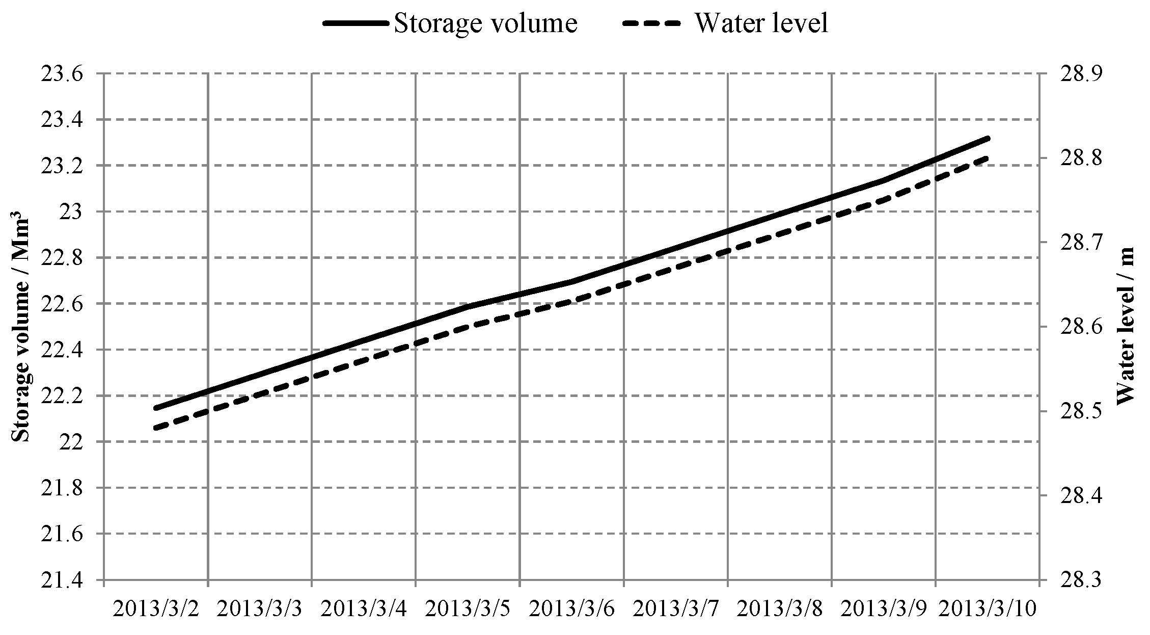
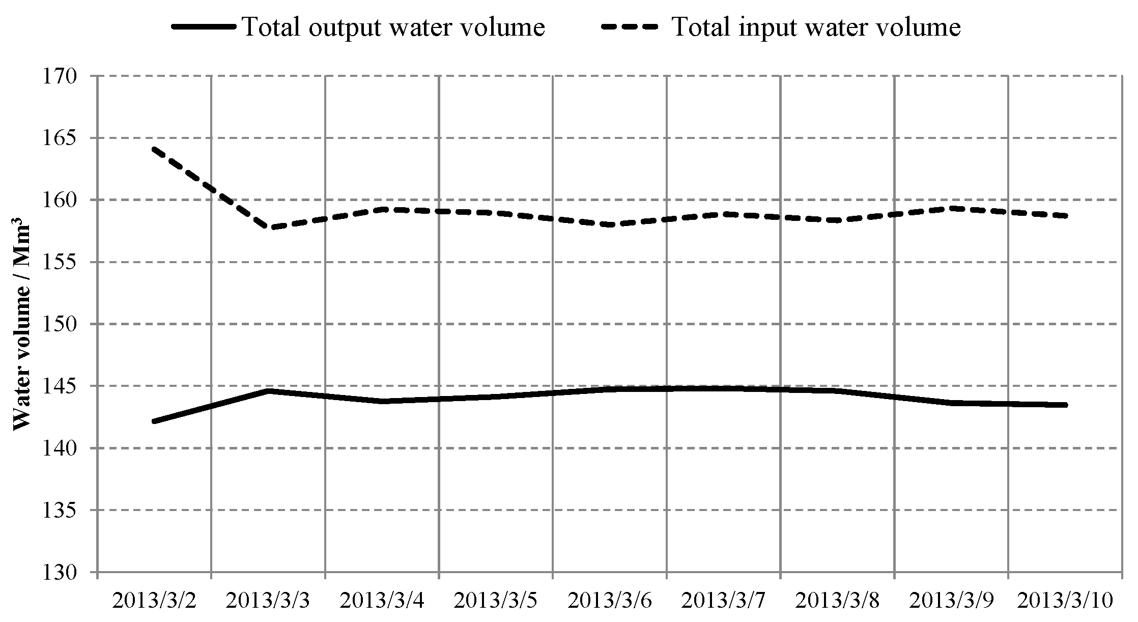
The operation process of the Xili reservoir from March 2, 2013 to March 10, 2013 is shown in

Table 5. The data results of the Xili reservoir during the dispatching process.

Item	2 March 2013	3 March 2013	4 March 2013	5 March 2013	6 March 2013	7 March 2013	8 March 2013	9 March 2013	10 March 2013
Rainfall (mm)	0	0	0	0	0	0	0	0	0
Water level (m)	28.48	28.52	28.56	28.6	28.63	28.67	28.71	28.75	28.8
Storage volume (104 m³)	2214.68	2229.32	2243.96	2258.6	2269.58	2284.22	2298.86	2313.5	2331.8
Increment or decrement of storage volume (104 m³)	21.96	14.64	14.64	14.64	10.98	14.64	14.64	14.64	18.3
Total water from outside (104 m³)	164.08	157.72	159.22	158.94	157.99	158.84	158.35	159.31	158.71
Runoff (104 m³)	0	0	0	0	0	0	0	0	0
Total water supply (104 m³)	142.15	144.59	143.75	144.13	144.72	144.81	144.59	143.62	143.45
Flood discharge volume (104 m³)	0	0	0	0	0	0	0	0	0
Transferred water to reservoir (104 m³)	0	0	0	0	0	0	0	0	0
Evaporation (104 m³)	0	0	0	0	0	0	0	0	0

, and Figure 9 and Figure 10. As can be seen from Figure 2, the Dongxi and Dachong waterworks are the water supply waterworks of the Xili reservoir, the Tiegang reservoir is the water supply reservoir, and the Dongbu mainline and Changpiling reservoir are the water sources of the Xili reservoir. In Table 5, the total water from outside means the amount of water diverted from the mainline and from other reservoirs, the total water supply means the amount of water supplied to the waterworks, and the transferred water to reservoir means the amount of water supplied to other reservoirs. From Table 5, and Figure 9 and Figure 10, it can be seen that the total water input of the Xili reservoir is larger than the total output during the operation period, so the reservoir is in the state of storing water, the reservoir’s water supply to the waterworks has not been interrupted, and the constraints (such as the water level and reservoir storage capacity) have also not been violated. In addition to this, during the operation period, the rainfall and runoff are zero, the reservoir is only used for the water supply, there is no discharge for the downstream river, and the reservoir evaporation is neglected in the calculation because of the unavailability of data.

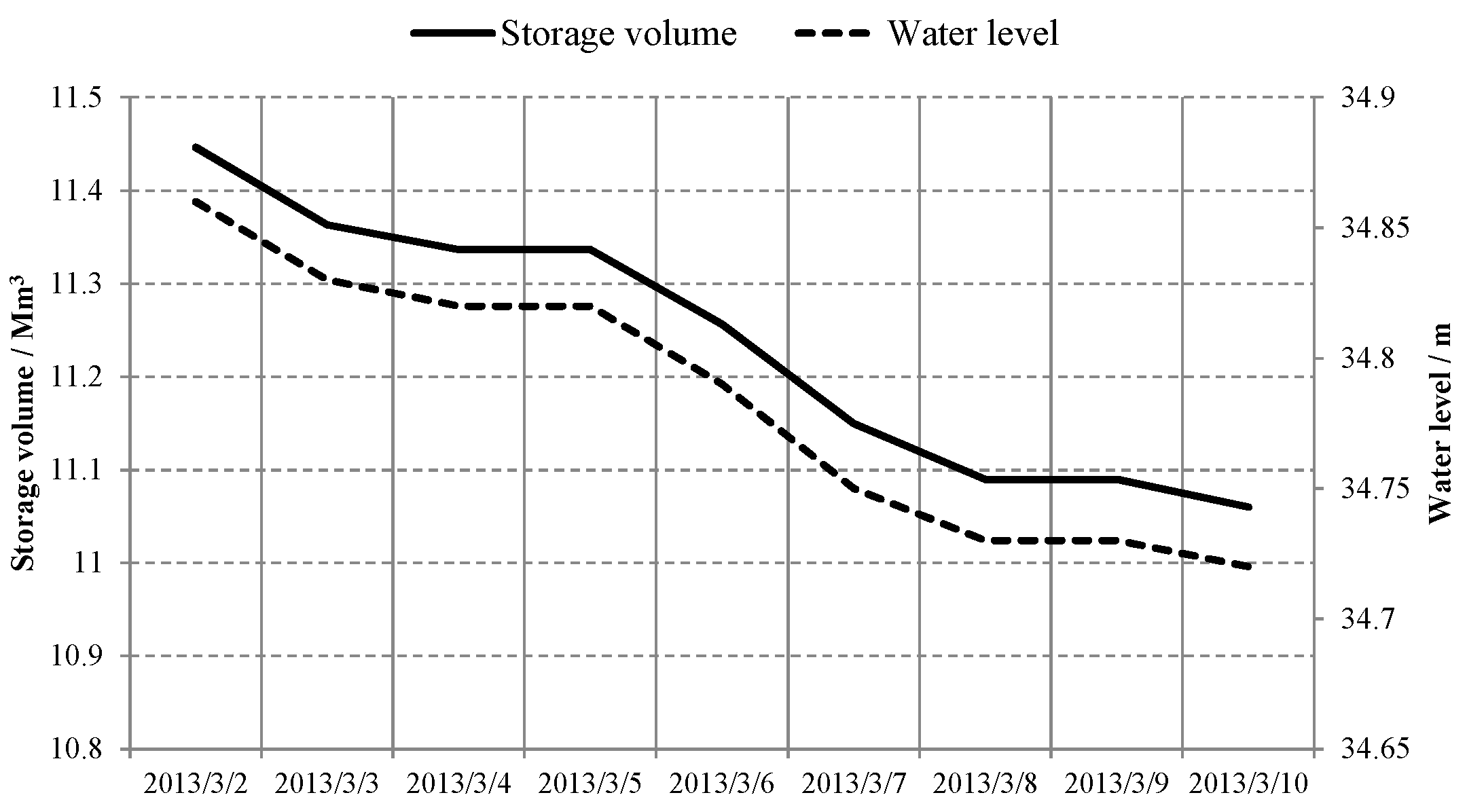
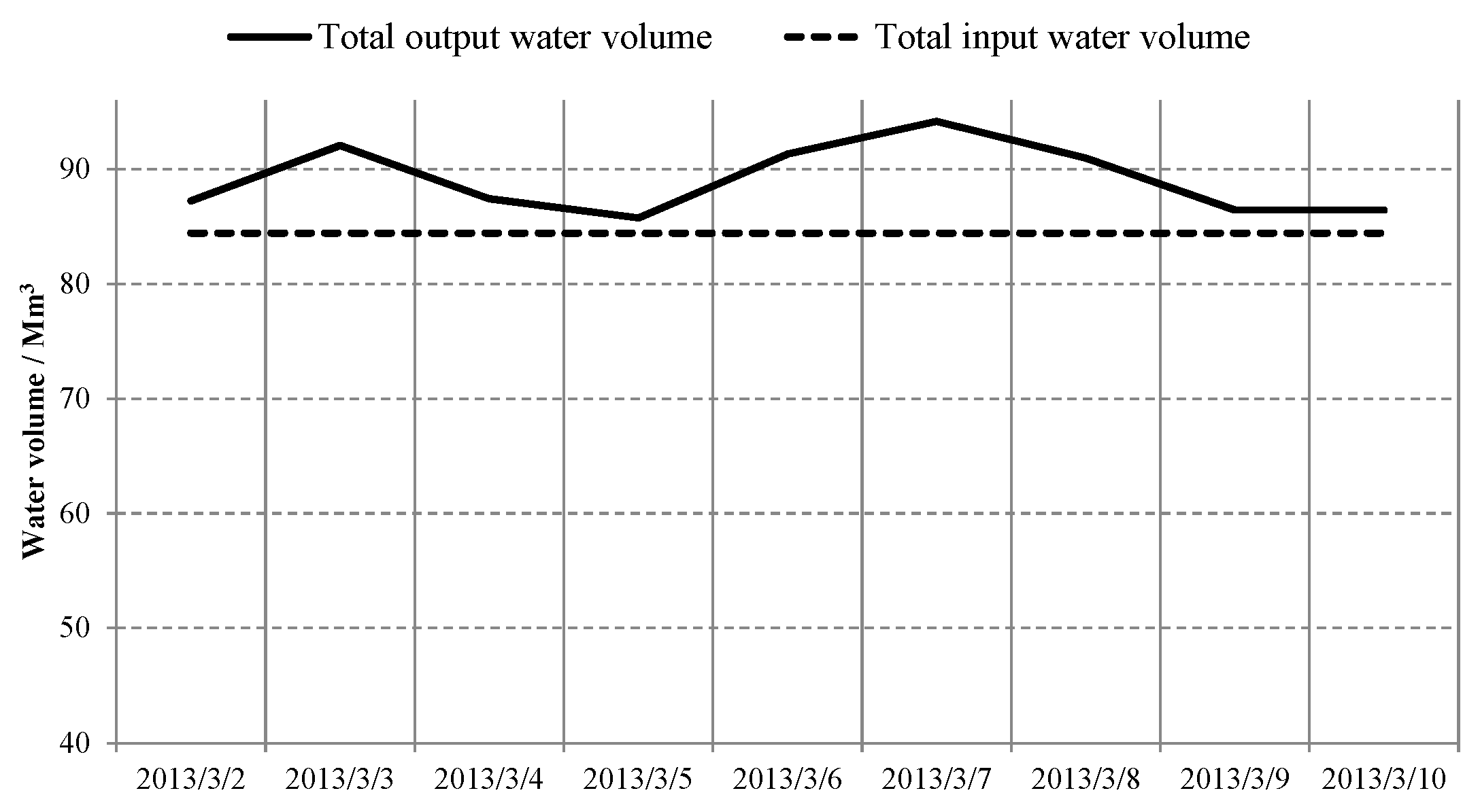
The operation process of the Shiyan reservoir from March 2, 2013 to March 10, 2013 is shown in

Table 6. The results of the Shiyan reservoir during the operation process.

Item	2 March 2013	3 March 2013	4 March 2013	5 March 2013	6 March 2013	7 March 2013	8 March 2013	9 March 2013	10 March 2013
Rainfall (mm)	0	0	0	0	0	0	0	0	0
Water level (m)	34.86	34.83	34.82	34.82	34.79	34.75	34.73	34.73	34.72
Storage volume (104 m³)	1144.67	1136.33	1133.67	1133.67	1125.67	1115	1109	1109	1106
Increment or decrement of storage volume (104 m³)	–2.83	–8.33	–2.67	0	–8	–10.67	–6	0	–3
Total water from outside (104 m³)	84.43	84.43	84.43	84.43	84.43	84.43	84.43	84.43	84.43
Runoff (104 m³)	0	0	0	0	0	0	0	0	0
Total water supply (104 m³)	87.25	92.05	87.44	85.75	91.32	94.18	90.95	86.43	86.43
Flood discharge volume (104 m³)	0	0	0	0	0	0	0	0	0
Transferred water to reservoir (104 m³)	0	0	0	0	0	0	0	0	0
Evaporation (104 m³)	0	0	0	0	0	0	0	0	0

, and in Figure 11 and Figure 12. According to Figure 2, the water supply waterworks of the Tiegang reservoir include the Xin’an waterworks, Zhuao waterworks, Shekou waterworks and Dachong waterworks. The water source is the Xili reservoir, and the water supply reservoir is the Shiyan reservoir (the Shiyan reservoir pumps water from the Tiegang reservoir through the Tieshi pumping station under conventional conditions, and the Shiyan reservoir discharges water through a spillway to the Tiegang reservoir under unconventional conditions). From Table 6, and from Figure 11 and Figure 12, it can be seen that the Shiyan reservoir is in a state of supplying water during the operation period under the constraints of the water level and reservoir capacity, that is, the daily water diversion is less than the daily water supply, but no violation occurs.

(2) Operation process of the key waterworks during the operation period.

Taking the Changliubi and Shiyan waterworks as examples, the operation processes of these key waterworks during the operation period are shown as follows.

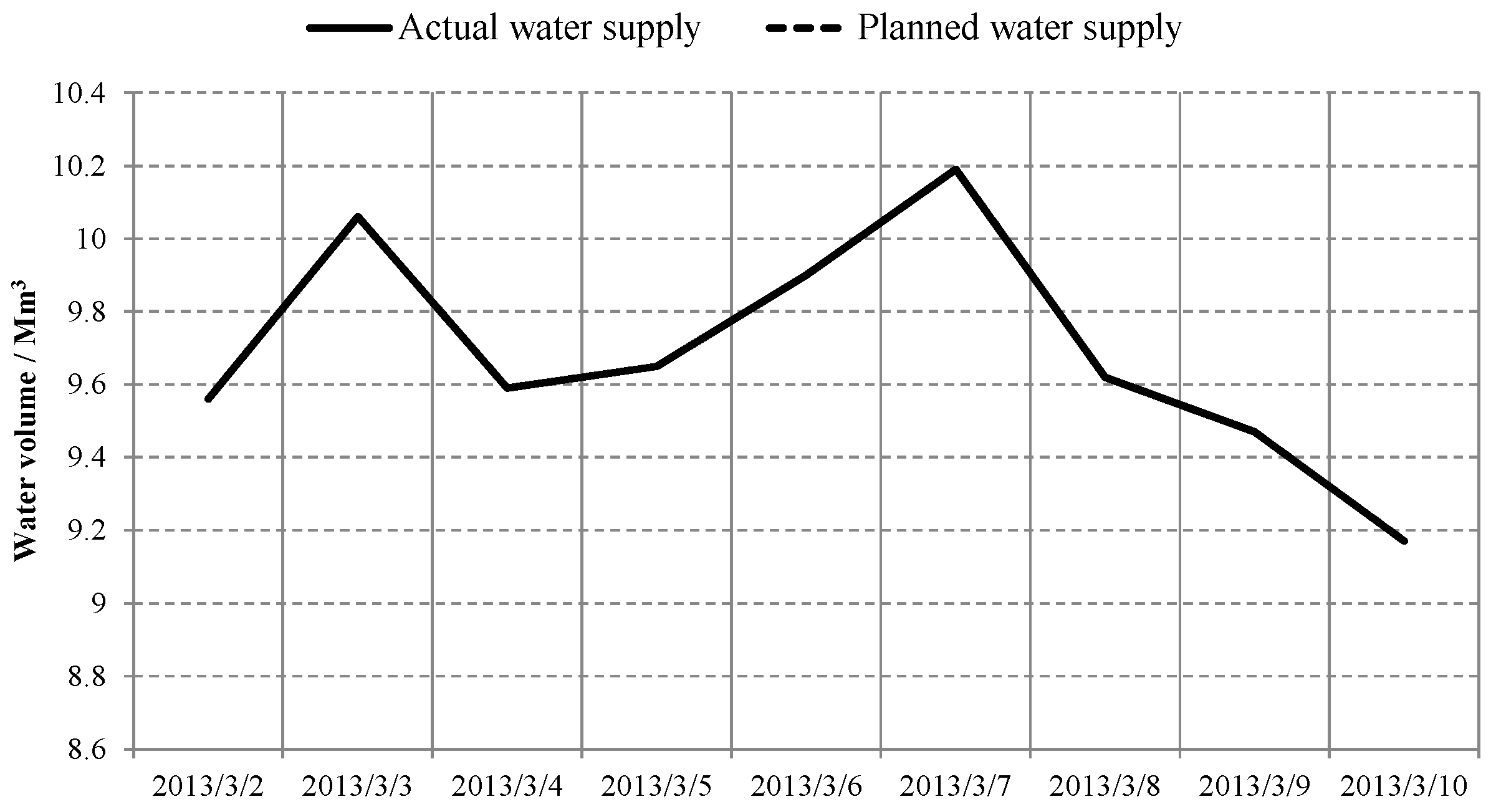
According to Figure 2, it can be seen that the water source of the Changliubi waterworks is the Changliubi and Shiyan reservoir. The water supply process of the Changliubi waterworks during the operation period is shown in

Table 7. The water dispatching process of the Changliubi waterworks.

Item	2 March 2013	3 March 2013	4 March 2013	5 March 2013	6 March 2013	7 March 2013	8 March 2013	9 March 2013	10 March 2013
Planned water supply (104m³)	20.23	21.81	19.7	19.54	22.2	23.44	21.19	19.5	18.99
Actual water supply (104m³)	20.23	21.81	19.7	19.54	22.2	23.44	21.19	19.5	18.99

and Figure 13. It can be seen that the planned water supply of this waterworks is exactly equal to the actual water supply during the operation period. Consequently, the water supply and demand of this waterworks are balanced, and the water supply satisfaction rate is 100% during this period.

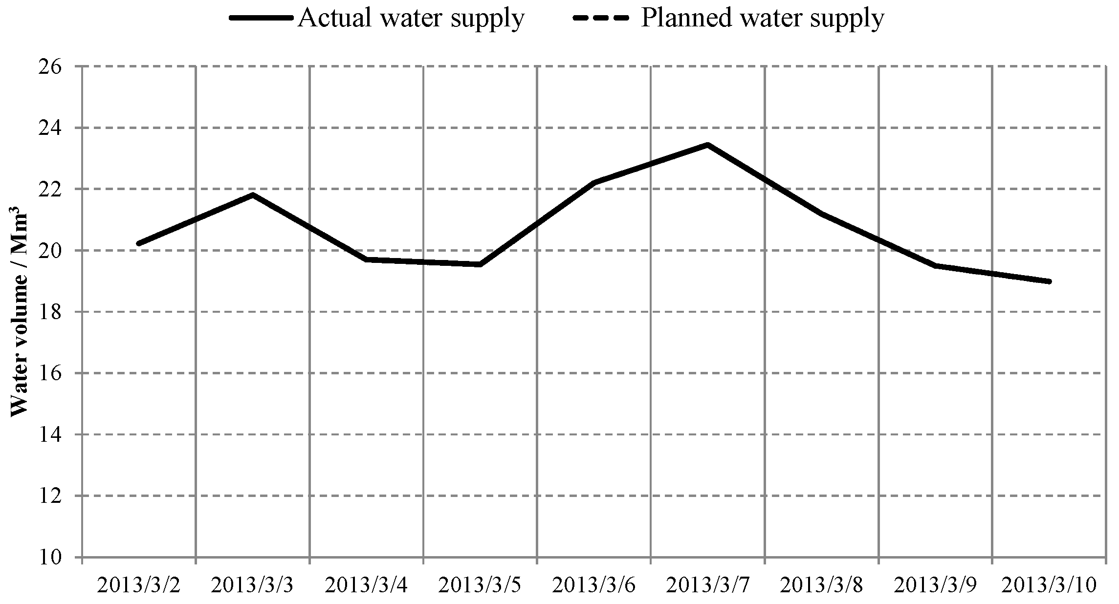
According to Figure 2, it can be seen that the water source of the Shiyan waterworks is the Shiyan reservoir, which is a single water source waterworks. The water supply process of the Shiyan waterworks during the operation period is shown in

Table 8. The water operation process of the Shiyan waterworks.

Item	2 March 2013	3 March 2013	4 March 2013	5 March 2013	6 March 2013	7 March 2013	8 March 2013	9 March 2013	10 March 2013
Planned water supply (104 m³)	9.56	10.06	9.59	9.65	9.9	10.19	9.62	9.47	9.17
Actual water supply (104 m³)	9.56	10.06	9.59	9.65	9.9	10.19	9.62	9.47	9.17

and Figure 14. It can be seen that the planned water supply of the Shiyan waterworks is exactly equal to the actual water supply during the operation period. Consequently, the water supply and demand of the Shiyan waterworks are balanced, and the water supply satisfaction rate is 100% during this period.

According to the subsystems determined in Figure 5, the water supply satisfaction rate of each waterworks in each subsystem is counted, and the results are shown in

Table 9. The statistical values of the water demand satisfaction rate of waterworks for each subsystem.

Item	Dongbu Mainline			Dongshen Mainline
Subsystem Index	Subsystem I	Subsystem III	Subsystem II	Subsystem IV	Subsystem VI	Subsystem V
Water supply satisfaction rate of waterworks	100%	99.5%	98.5%	100.0%	98.1%	100.0%

. It can be seen that the guaranteed rate of each subsystem is over 97%. Therefore, the water demand of the whole city’s waterworks has basically been well met during the operation period. Here, not all of the water demands are 100% satisfied, mainly because there are some single source waterworks in the system, and the water source of these waterworks is also not linked with the Dongshen or the Dongbu mainline, so the water demand cannot be supplemented during some stages. This applies, for example, to the Jingzi waterworks in subsystem II, Wutongshan waterworks, Meisha and Yanluo waterworks in subsystem III, Tangkeng waterworks in subsystem VI, etc.

Generally speaking, the raw water allocation in Shenzhen based on the model proposed in this paper can meet the water demand and ensure the normal water supply of each waterworks.

(3) Budget analysis of the water resources management units.

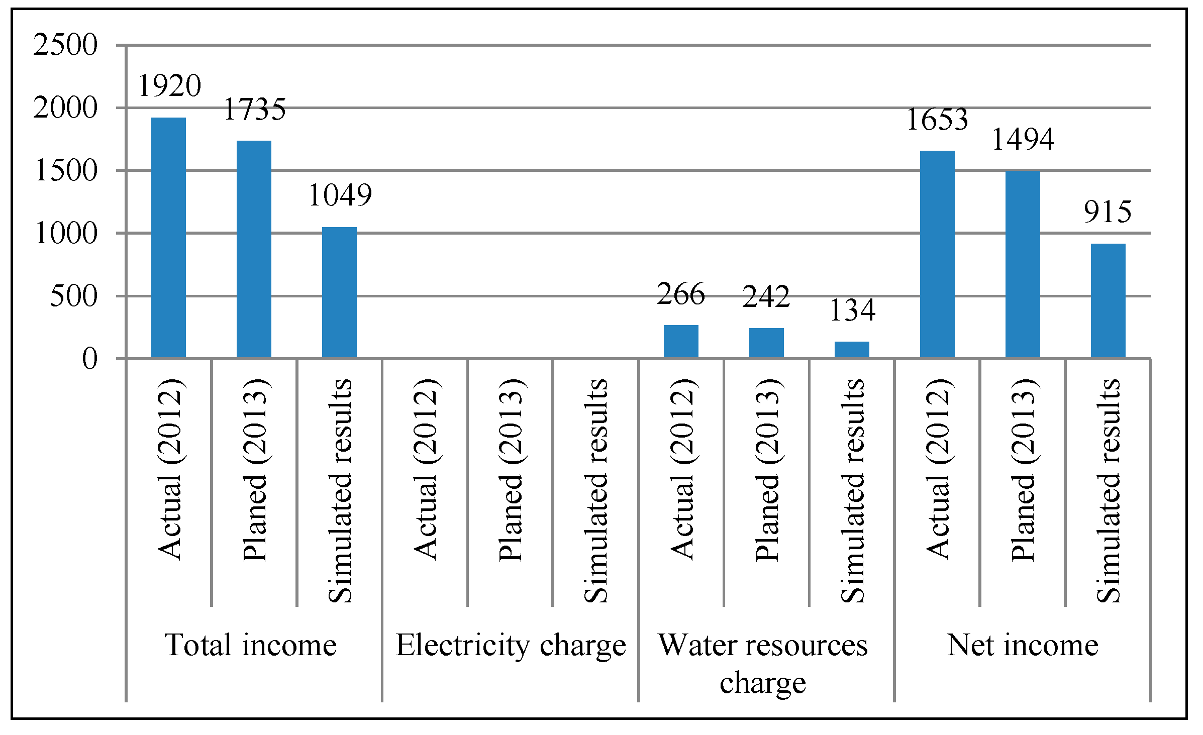
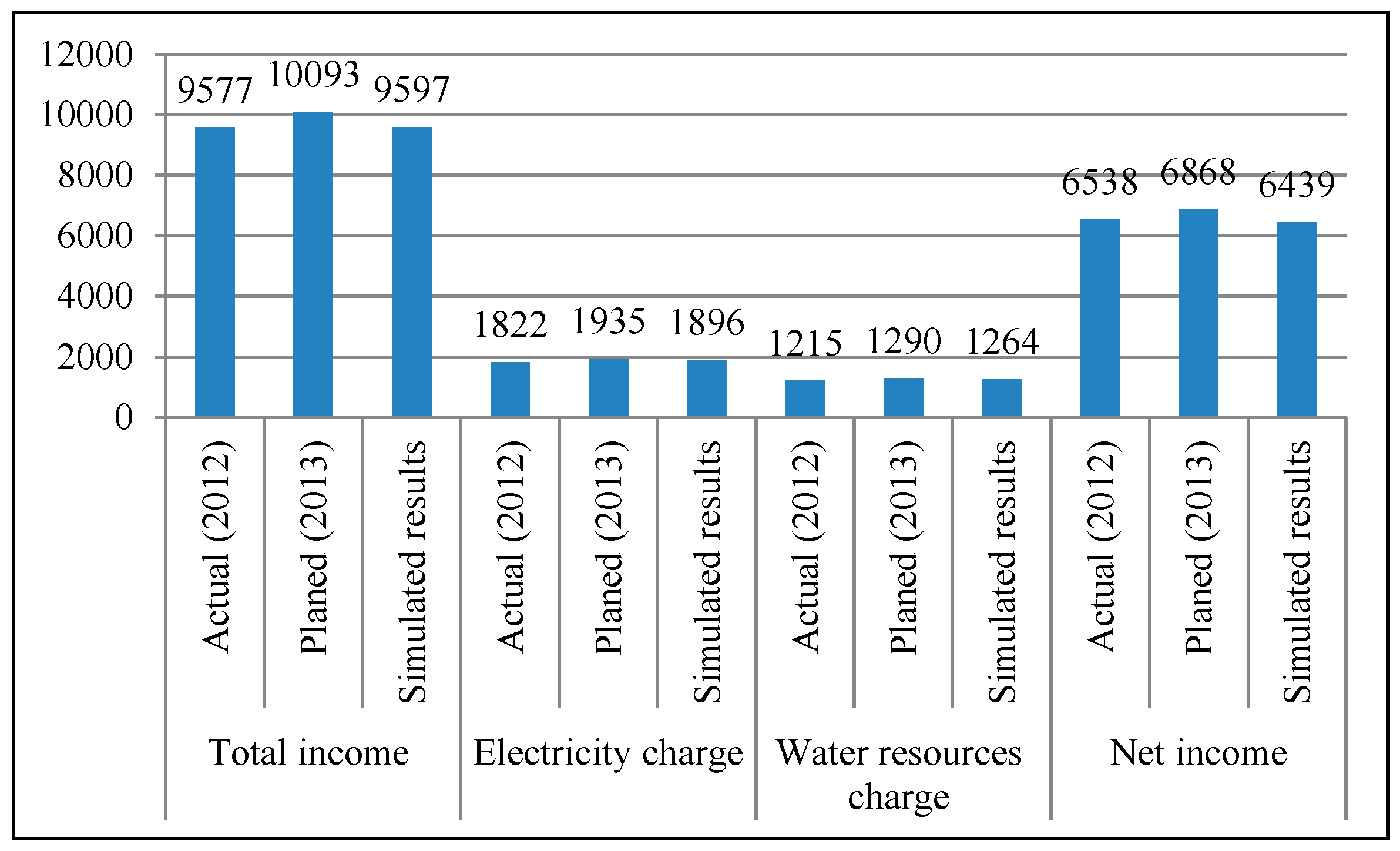
In the process of solving the model, the budget balance requirement of each water resources management unit can be further considered. In order to compare with the actual operation in March 2–10 in 2012 and the planned operation in March 2–10 in 2013, this paper uses the same boundary conditions and initial conditions to calculate the scheme with the model. After the iteration calculation of different levels of objectives, the scheduling scheme considering the budget target of water resources management units is obtained. According to the statistics of the actual and planned operation scheme during March 2–10 and the simulation operation scheme of this model, the budget situation of each management unit is obtained, as shown in

Table 10. The total income, electricity charge, water resources charge and net income of four water management units during the period of 2–10 March under three situations (Actual 2012, Planned 2013, Simulated results).

Index	Situation	Dongshen	Dongbu	Tieshi	Beibu
Total income/104 yuan	Actual (2012)	1920	9577	6445	4625
	Planned (2013)	1735	10,093	6413	4564
	2–10 March	1049	9597	5889	2445
Electricity charge/104 yuan	Actual (2012)	---	1822	722	962
	Planned (2013)	---	1935	756	935
	2–10 March	---	1896	879	136
Water resources charge/104 yuan	Actual (2012)	266	1215	5547	4221
	Planned (2013)	242	1290	5921	4103
	2–10 March	134	1264	4544	601
Net income/104 yuan	Actual (2012)	1653	6538	177	–557
	Planned (2013)	1494	6868	–264	–472
	2–10 March	915	6439	466	1707

. Where the total income represents the gross income of the water supply, the electricity charge refers to the electricity cost of the pumping station for water lifting. The Dongshen mainline spends zero electricity costs because all the water is self-flowing during the operation period and no water lifting is needed. Water resources charges are paid to intake water from external water sources. The net income means the total income minus the electricity charge and water resources charge. In addition, depreciation losses of the pumping stations, gates and pipelines are not taken into account in the calculation. Tips: the exchange rate of RMB to USD is 6.72 in March 2013, and the exchange rate of USD to RMB is 0.1488.

The total income, electricity charge, water resources charge and net income of the four water management units during the period of 2–10 March under three conditions (Actual 2012, Planned 2013, Simulated results) are shown in Figure 15, Figure 16, Figure 17 and Figure 18, respectively. Overall, from the four figures, it can be seen that the total income, expenditure on electricity, water resources charge, and net income of the Dongbu and Tieshi units in the period of 2–10 March are similar in the three situations, and the budget is basically consistent with the simulation results, while the four indicators of the other two water management units (Dongshen and Beibu) are quite different in the three situations.

In addition, for Tieshi and Beibu, it can be seen that the total income of the simulated results decreased when compared with Actual 2012 and Planned 2013, but the net income increased. The main reason for this is that, compared with Actual 2012 and Planned 2013, the expenditure on electricity and water resources of the simulated results has decreased, especially the water resources fee of Tieshi, which has been reduced from 5921 in Planned 2013 to 4544 in the simulated calculation, and the expenditures on the electricity and water resources fee of Beibu, which have been reduced, respectively, from 935 in Planned 2013 to 136 in the simulated calculation, and from 4103 in Planned 2013 to 601 in the simulated calculation. From this result, it can be seen that the model and the solving method proposed in this paper can solve the problem of raw water allocation in Shenzhen very well, and that it can consider and basically maintain the budget balance of the water resources management units in the model calculation. In addition, under the same boundary conditions, this model can effectively reduce the expenditure of electricity and water resources, and increase the net income of the water supply system through the optimization.

Compared with the research results of other literatures, such as [27], the authors also studied the balance between the supply and demand of water resources in Shenzhen, and established a system dynamics model by which the water supply and demand in Shenzhen City was simulated from 2015 to 2030, and some meaningful conclusions had been achieved. However, the complexity of Shenzhen’s water supply system was not described and modeled in this literature, and only the balance between the supply and demand of the water volume was studied, while the department budget was not discussed. In the literature [42], in order to improve the water supply security better in terms of the water quality and quantity in the water system, the authors adopted the method of decomposition and coordination of a large-scale system; by integrating the optimal operation of the water quantity, water quality simulation and strategy analysis of the water quality control, they established a water quality and quantity control coupling model for Shenzhen’s water supply system. The application results proved that the model proposed in this paper was feasible and effective, offering a new method to improve the raw water quality supply security. However, in this literature, only 7 key reservoirs and 21 waterworks in Shenzhen were studied. A large number of existing reservoirs and waterworks that have a mutual influence with each other were not considered, and the degree of simplification was relatively large, making the system scale much smaller than the system scale in this paper. Consequently, by contrast, the research of Shenzhen’s water supply system is not only huge in scale in this paper, but also more comprehensive in targets and factors, which has a greater practical application value.

5. Conclusions

In this paper, the raw water allocation problem of Shenzhen City is taken as the research object. Through the generalization and description of a one-to-many, many-to-one complex network relationship in this system, the network topology of the water source supply system is established, which includes 46 reservoirs, 67 waterworks, 2 external diversion water sources, 14 pumping stations and 9 gates. Combining the forecasting model of the water demand of waterworks and aimed at meeting the guaranteed rate requirement of the water supply of a multi-sources system, a water allocation model for large-scale cities is established. Based on this model, the raw water allocation problem in Shenzhen is studied in depth, and the following conclusions are drawn.

(1) The double-layer feedback mechanism proposed in this paper, which takes the reverse calculation mode as the outer feedback and the reservoir water level or pipeline capacity constraint as the inner feedback, can solve the water allocation problem of a complex water supply system in large cities very well, and has an important application value and practical significance.

(2) Taking Shenzhen as an example, the research in this paper not only realizes the generalization of a complex water supply network that includes 46 reservoirs, 67 waterworks and 14 pumping stations, but it also realizes the scientific and rational allocation of water resources in a large-scale complex water supply system through the proposed model.

(3) The case study shows that under the same boundary conditions, compared with the original plan, the proposed model can effectively reduce the expenditure on electricity and water resources, and improve the net income of the water supply system.

Of course, there are still some shortcomings in the current research work. For example, after obtaining the water allocation scheme that meets the requirement on the guaranteed rate, the unfinished work of this paper is how to further reduce the cost of the scheme on the basis of the budget balance of the water resources management units, so as to optimize the economic performance of the scheme, and this is also the focus of our next work.

References

- Qin, X.; Xu, Y. Analyzing urban water supply through an acceptability-index-based interval approach. Adv. Water Resour. 2011, 34, 873–886. [Google Scholar] [CrossRef]
- Đurin, B.; Margeta, J. Analysis of the Possible Use of Solar Photovoltaic Energy in Urban Water Supply Systems. Water 2014, 6, 1546–1561. [Google Scholar] [CrossRef] [Green Version]
- Hong, X.; Guo, S.; Wang, L.; Yang, G.; Liu, D.; Guo, H.; Wang, J. Evaluating Water Supply Risk in the Middle and Lower Reaches of Hanjiang River Basin Based on an Integrated Optimal Water Resources Allocation Model. Water 2016, 8, 364. [Google Scholar] [CrossRef]
- Li, S.; Chen, X.; Singh, V.P.; He, Y. Assumption-Simulation-Feedback-Adjustment (ASFA) Framework for Real-Time Correction of Water Resources Allocation: a Case Study of Longgang River Basin in Southern China. Water Resour. Manag. 2018, 32, 3871–3886. [Google Scholar] [CrossRef] [Green Version]
- Liu, D.; Guo, S.; Liu, P.; Zou, H.; Hong, X. Rational Function Method for Allocating Water Resources in the Coupled Natural-Human Systems. Water Resour. Manag. 2018, 33, 57–73. [Google Scholar] [CrossRef]
- Abdulbaki, D.; Al-Hindi, M.; Yassine, A.; Najm, M.A. An optimization model for the allocation of water resources. J. Clean. Prod. 2017, 164, 994–1006. [Google Scholar] [CrossRef]
- Ahmad, A.; El-Shafie, A.; Razali, S.F.M.; Mohamad, Z.S. Reservoir Optimization in Water Resources: a Review. Water Resour. Manag. 2014, 28, 3391–3405. [Google Scholar] [CrossRef]
- Jiang, Z.; Qin, H.; Ji, C.; Hu, D.; Zhou, J. Effect Analysis of Operation Stage Difference on Energy Storage Operation Chart of Cascade Reservoirs. Water Resour. Manag. 2019. [Google Scholar] [CrossRef]
- Men, B.; Liu, H.; Tian, W.; Liu, H. Evaluation of Sustainable Use of Water Resources in Beijing Based on Rough Set and Fuzzy Theory. Water 2017, 9, 852. [Google Scholar] [CrossRef]
- Jiang, Z.; Wu, W.; Qin, H.; Zhou, J. Credibility theory based panoramic fuzzy risk analysis of hydropower station operation near the boundary. J. Hydrol. 2018, 565, 474–488. [Google Scholar] [CrossRef]
- Gutie´rrez-Martin, C.; Borrego-Marin, M.M.; Berbel, J. The Economic Analysis of Water Use in the Water Framework Directive Based on the System of Environmental-Economic Accounting for Water: A Case Study of the Guadalquivir River Basin. Water 2017, 9, 180. [Google Scholar] [CrossRef]
- Sigvaldson, O.T. A simulation model for operating a multipurpose multireservoir system. Water Resour. Res. 1976, 12, 263–278. [Google Scholar] [CrossRef]
- Jiang, Z.; Ji, C.; Qin, H.; Feng, Z. Multi-stage progressive optimality algorithm and its application in energy storage operation chart optimization of cascade reservoirs. Energy 2018, 148, 309–323. [Google Scholar] [CrossRef]
- Mass, A.; Hufschmidt, M.M.; Dorfman, R.; Thomas, H.A., Jr.; Marglin, S.A.; Fair, G.M. Design of Water Resource Management; Harvard University Press: Cambridge, MA, USA, 1962. [Google Scholar]
- Haimes, Y.Y.; Allee, D.J. Multi-Objective Analysis in Water Resources; Ameriean Soeiety of Civil Engineers: New York, NY, USA, 1982. [Google Scholar]
- Labadie, J.W.; Bode, D.; Pineda, A. Network Model for Decision-Support Simulate Palraw Water Supply. Water Resour. Bull. 1986, 22, 927–940. [Google Scholar] [CrossRef]
- Kumar, K.S.; Galkate, R.V.; Tiwari, H.L. River basin modelling for Shipra River using MIKE BASIN. Ish J. Hydraul. Eng. 2018, in press. [Google Scholar] [CrossRef]
- McKinney, D.C.; Cai, X.M. Linking GIS and water Resource Management models: a method. Environ. Modeling Softw. 2002, 17, 413–425. [Google Scholar] [CrossRef]
- Zhao, J.; Wang, Z.; Weng, W. Theory and Model of Water Resources Complex Adaptive Allocation System. J. Geogr. Sin. 2003, 13, 112–122. [Google Scholar] [CrossRef]
- Willis, R.; Yeh, W.W. Ground Water System Planning and Management; Prentice-Hall: Upper Saddle River, NJ, USA, 1987. [Google Scholar]
- Watkins, D.W., Jr.; Daene, C.M. Optimization for incorporating risk and uncertainty in sustainable water resources planning. Int. Assoc. Hydrol. Sci. 1995, 231, 225–232. [Google Scholar]
- Jiang, Z.; Qiao, Y.; Chen, Y.; Ji, C. A New Reservoir Operation Chart Drawing Method Based on Dynamic Programming. Energies 2018, 11, 3355. [Google Scholar] [CrossRef]
- Jiang, Z.; Qin, H.; Wu, W.; Qiao, Y. Studying Operation Rules of Cascade Reservoirs Based on Multi-Dimensional Dynamics Programming. Water 2017, 10, 20. [Google Scholar] [CrossRef]
- Jiang, Z.; Qin, H.; Ji, C.; Feng, Z.; Zhou, J. Two Dimension Reduction Methods for Multi-Dimensional Dynamic Programming and Its Application in Cascade Reservoirs Operation Optimization. Water 2017, 9, 634. [Google Scholar] [CrossRef]
- Merabtene, T.; Kawamura, A.; Jinno, K.; Olsson, J. Risk assessment for optimal drought management of an integrated water resources system using a genetic algorithm. Hydrol. Process. 2010, 16, 2189–2208. [Google Scholar] [CrossRef]
- Feng, Z.-K.; Niu, W.-J.; Cheng, C.-T. Optimization of hydropower reservoirs operation balancing generation benefit and ecological requirement with parallel multi-objective genetic algorithm. Energy 2018, 153, 706–718. [Google Scholar] [CrossRef]
- Li, Y.; Zhao, T.; Wang, P.; Gooi, H.B.; Wu, L.; Liu, Y.; Ye, J.; Li, Y. Optimal Operation of Multimicrogrids via Cooperative Energy and Reserve Scheduling. IEEE Trans. Ind. Inform. 2018, 14, 3459–3468. [Google Scholar] [CrossRef]
- Afshar, A.; Shojaei, N.; Sagharjooghifarahani, M. Multiobjective Calibration of Reservoir Water Quality Modeling Using Multiobjective Particle Swarm Optimization (MOPSO). Water Resour. Manag. 2013, 27, 1931–1947. [Google Scholar] [CrossRef]
- Liu, Y.; Qin, H.; Mo, L.; Wang, Y.; Chen, D.; Pang, S.; Yin, X. Hierarchical Flood Operation Rules Optimization Using Multi-Objective Cultured Evolutionary Algorithm Based on Decomposition. Water Resour. Manag. 2019, 33, 337–354. [Google Scholar] [CrossRef]
- Lu, H.; Guo, Y.; Sheng, P. Study on decomposition-coordination decision model of the water resources system in Yiwu City. J. Hydraul. Eng. 1997, 6, 40–47. [Google Scholar]
- Wang, M.; Zheng, C. Ground water management optimization using genetic algorithms and simulated annealing: formulation and comparison. Jawra J. Am. Water Resour. Assoc. 1998, 34, 519–530. [Google Scholar] [CrossRef]
- Teegavarapu, R.S.V.; Simonovic, S.P. Optimal operation of reservoir simulated annealing. Water Resour. Manag. 2002, 16, 401–428. [Google Scholar] [CrossRef]
- Li, T.; Yang, S.; Tan, M.; Tianhong, L.; Songnan, Y.; Mingxin, T. Simulation and optimization of water supply and demand balance in Shenzhen: A system dynamics approach. J. Clean. Prod. 2018, 207, 882–893. [Google Scholar] [CrossRef]
- Willuweit, L.; O’Sullivan, J.J. A decision support tool for sustainable planning of urban water systems: Presenting the Dynamic Urban Water Simulation Model. Water Res. 2013, 47, 7206–7220. [Google Scholar] [CrossRef] [PubMed]
- Fang, W.; Huang, S.; Ren, K.; Huang, Q.; Huang, G.; Cheng, G.; Li, K. Examining the applicability of different sampling techniques in the development of decomposition-based streamflow forecasting models. J. Hydrol. 2019, 568, 534–550. [Google Scholar] [CrossRef]
- Jiang, Z.; Wu, W.; Qin, H.; Hu, D.; Zhang, H. Optimization of fuzzy membership function of runoff forecasting error based on the optimal closeness. J. Hydrol. 2019, 570, 51–61. [Google Scholar] [CrossRef]
- Li, R.; Jiang, Z.; Ji, C.; Li, A.; Yu, S. An improved risk-benefit collaborative grey target decision model and its application in the decision making of load adjustment schemes. Energy 2018, 156, 387–400. [Google Scholar] [CrossRef]
- Meng, E.; Huang, S.; Huang, Q.; Fang, W.; Wu, L.; Wang, L. A robust method for non-stationary streamflow prediction based on improved EMD-SVM model. J. Hydrol. 2019, 568, 462–478. [Google Scholar] [CrossRef]
- Jiang, Z.; Li, R.; Li, A.; Ji, C. Runoff forecast uncertainty considered load adjustment model of cascade hydropower stations and its application. Energy 2018, 158, 693–708. [Google Scholar] [CrossRef]
- Feng, Z.; Niu, W.; Cheng, C. China’s large-scale hydropower system: operation characteristics, modeling challenge and dimensionality reduction possibilities. Renew. Energy 2019, 136, 805–818. [Google Scholar] [CrossRef]
- Niu, W.; Feng, Z.; Feng, B.; Min, Y.; Cheng, C.; Zhou, J. Comparison of multiple linear regression, artificial neural network, extreme learning machine and support vector machine in deriving hydropower reservoir operation rule. Water 2019, 11, 88. [Google Scholar] [CrossRef]
- Zhao, B.; Wang, L.; Zhang, Y.; Liu, F. Study on the coupling model for water quality and quantity control in the urban raw water system. Shuili Xuebao 2012, 40, 1373–1380. [Google Scholar]
Figure 1.
The distribution of the actual reservoirs, waterworks, pumping stations, gates and water supply pipelines in Shenzhen City.
Figure 2.
Generalization chart of the water supply system in Shenzhen.
Figure 3.
The water demand forecasting process of the waterworks.
Figure 4.
The flowchart of water allocation of the waterworks.
Figure 5.
The hierarchical structure of the large-scale system decomposition model.
Figure 6.
The core calculation process of the forward calculation mode.
Figure 7.
The core calculation flowchart of the reverse calculation mode.
Figure 8.
The double-layer feedback regulation based solving process of the dynamic simulation of the supply-demand balance.
Figure 9.
The water level process of the Xili reservoir during the operation.
Figure 10.
The water volume process of the Xili reservoir during the operation.
Figure 11.
The water level process of the Tieshi reservoir during the operation.
Figure 12.
The water volume process of the Tieshi reservoir during the operation period.
Figure 13.
The water flow process of the Changliubi waterworks during the operation period.
Figure 14.
The water flow process of the Shiyan waterworks during the operation period.
Figure 15.
The total income, water resources fee and net income of Dongshen during the period from 3.2 to 3.10 under different situations (unit: 104 yuan).
Figure 16.
The total income, water resources fee and net income of Dongbu during the period from 3.2 to 3.10 under different situations (unit: 104 yuan).
Figure 17.
The total income, water resources fee and net income of Tieshi during the period from 3.2 to 3.10 under different situations (unit: 104 yuan).
Figure 18.
The total income, water resources fee and net income of Beibu during the period from 3.2 to 3.10 under different situations (unit: 104 yuan).