Experimental Investigations and CFD Modeling of Contaminant Intrusion in a Water Network during Transient Events

Abstract

Intrusion in drinking water networks (DWN) can be triggered by transient low-pressure events. This intrusion may result in the contamination of drinking water supplied to consumers, which may have major health impacts. This research aims to investigate the influence of a DWN’s operating parameters on the intrusion and progression of the contaminant in a pilot drinking water network setup. Results show that the minimum time required for the contaminant to begin entering the system was influenced by the system operating pressure. Faster initial intrusion times were observed under low operating pressure. In addition, the crack size influenced the time required for the contaminant to fully intrude the system. Similarly, the time required for the contaminant to reach certain points in the DWN was influenced by the operating pressure. These results were verified using two additional tools; a high-speed camera was used to monitor the contaminant transient progression through the DWN under different pressures; and computational fluid dynamics modeling was used to calculate the corresponding contaminant concentration. The results suggest that the ability of the system to quickly stabilize its operating pressure would reduce the probability of a contaminant intrusion into the DWN.

1. Introduction

Many local governments and municipalities maintain their drinking water network (DWN) by continuous inspection of water mains, tanks, pipes, and junctions [1]. Local governmental authorities, as well as international regulations and standards, usually set guidelines and standards for maintaining and monitoring water quality in DWNs. Water quality in the distribution network can be defined by several standard microbiological, physicochemical, and aesthetic indicators or parameters [2].

Typically, water quality testing is performed at water treatment plants. However, often due to budget limitations, water quality monitoring in the DWN receives less attention [3]. Nevertheless, contamination in the distribution networks can have severe impacts on consumers’ health as there is usually little treatment implemented in the form of residual disinfectant boosters once water enters the DWN for delivery to the end users [1]. In many cases, it is difficult to monitor water quality in the DWN because water is usually transferred very quickly from the source to consumers, which could result in severe community health impacts in the event of accidental or deliberate water contamination.

Water contamination in a DWN can cause major health impacts [4]. Over the past few decades, several events have occurred and have sounded the alarm for the risks from such contamination; an example is the Salmonella typhimurium contamination in the water supply system in Missouri [5] that caused illness to more than 400,000 people [4]. Other events include the presence of Lead (Pb) in the DWN and the resulting severe impact on the hemopoietic, nervous, endocrine, and cardiovascular systems in the human body [6]. In addition, studies done on arsenic have shown that long-term exposure from drinking water can cause cancer in skin, lungs, bladder, and kidneys [7,8,9,10]. Other studies have reported a direct connection between cases of diarrhea and low, negative pressure events or contamination events [11], which raises concerns regarding possible health impacts, especially among young children. Many studies focused on optimizing booster chlorination in DWNs [12,13]. However, possible transient pressure incidents could increase the risk of contaminant ingress, which needs to be taken into account during DWN’s water quality management [14].

There are many factors (such as pipe material, operating pressure, and pipe age) influencing the potential for water leaks and contaminant intrusion in a DWN [15,16,17,18,19,20]. The choice of water pipe material (ex. PVC, asbestos-cement (AC), concrete (CONC), ductile iron (DI), and cast iron (CI)) can greatly affect the potential for pipe deterioration and resistance to stresses which consequently influences the potential for cracks and leaks [21,22]. In general, aged pipes have a higher potential for cracks and leaks and the consequent contaminant intrusion in a DWN [15,16]. For example, leakage rates from DWNs were found to be at least 10% in Dubai, United Arab Emirates and can reach to as high as approximately 56% in Makkah, Kingdom of Saudi Arabia [15,16]. Leaks resulting from pinholes, cracks, and joint/connection failures are possible pathways through which contaminants may enter the DWN. Such leaks can be classified as either background leaks or bursts based on their size [17]. The surrounding contaminants cannot intrude the pipe unless the water main pressure is very low or negative [18,19]. Previous research determined that transient negative pressure periods and contaminant concentration in the area surrounding the DWN can directly affect the intrusion process [20]. Factors that can affect intrusion include pressure changes around the crack area, the surrounding environmental conditions [23,24], the re-intrusion of water that was lost during the leak process, and the nature of the flow through the orifice (crack) and its driving force [25]. An analytical relationship was given in [26] to combine the seepage in soil and the flow through an orifice to predict the intrusion flow rate for a circular orifice under steady-state conditions. The experimental quantification of intrusion due to transients using a large-scale system shows that the volume of intrusion is connected to the duration and magnitude of the negative pressure transient [27]. Fox et al., [25,28] have also reported that short duration, oscillating (but extreme) transient pressure events can result in contaminant intrusion with the ingress volume having an inverse relationship with the distance of the contaminant from the leak.

Other studies have examined contamination in DWNs due to the presence of leakage during transients with negative pressure or during periods in which pipes are partially empty [29]. These studies concluded that pipeline leaks during negative pressure events provided a potential entry path of groundwater into treated drinking water [20,23]. Following intrusion, contaminant transport is also affected by the DWN design, the operating pressure, the duration of low or negative pressure (the driving force), and the sources of contamination surrounding the pipes [23,26]. An experimental plumbing rig designed to replicate the range of pressures encountered in an actual small network system was presented in [20,30] to address how a pressure transient triggered within a house or in a municipal system could impact the service line with a possible suction effect. Although there is a wide agreement that contaminant ingress is associated with incidents of low or negative pressure [23,26], additional research is required to understand how far contaminants can travel within a DWN under different low-pressure conditions.

It is difficult to carry out experimental studies on real DWNs due to issues of safety and public health safeguard [24]. Creating representative laboratory networks is costly and technically challenging [31]; small experimental setups, however, can still represent a case of a pilot drinking water network. They could be sufficient to investigate the influence of operating parameters on the intrusion and progression of the contaminant in the DWN. In this paper, for the first time, a combination of a physical experimental setup and modeling using computational fluid dynamics (CFD) was used to investigate the effect of operating pressure and crack features on the extent and speed of contaminant intrusion, its transport, and concentration within a DWN during low-pressure events.

2. Materials and Methods

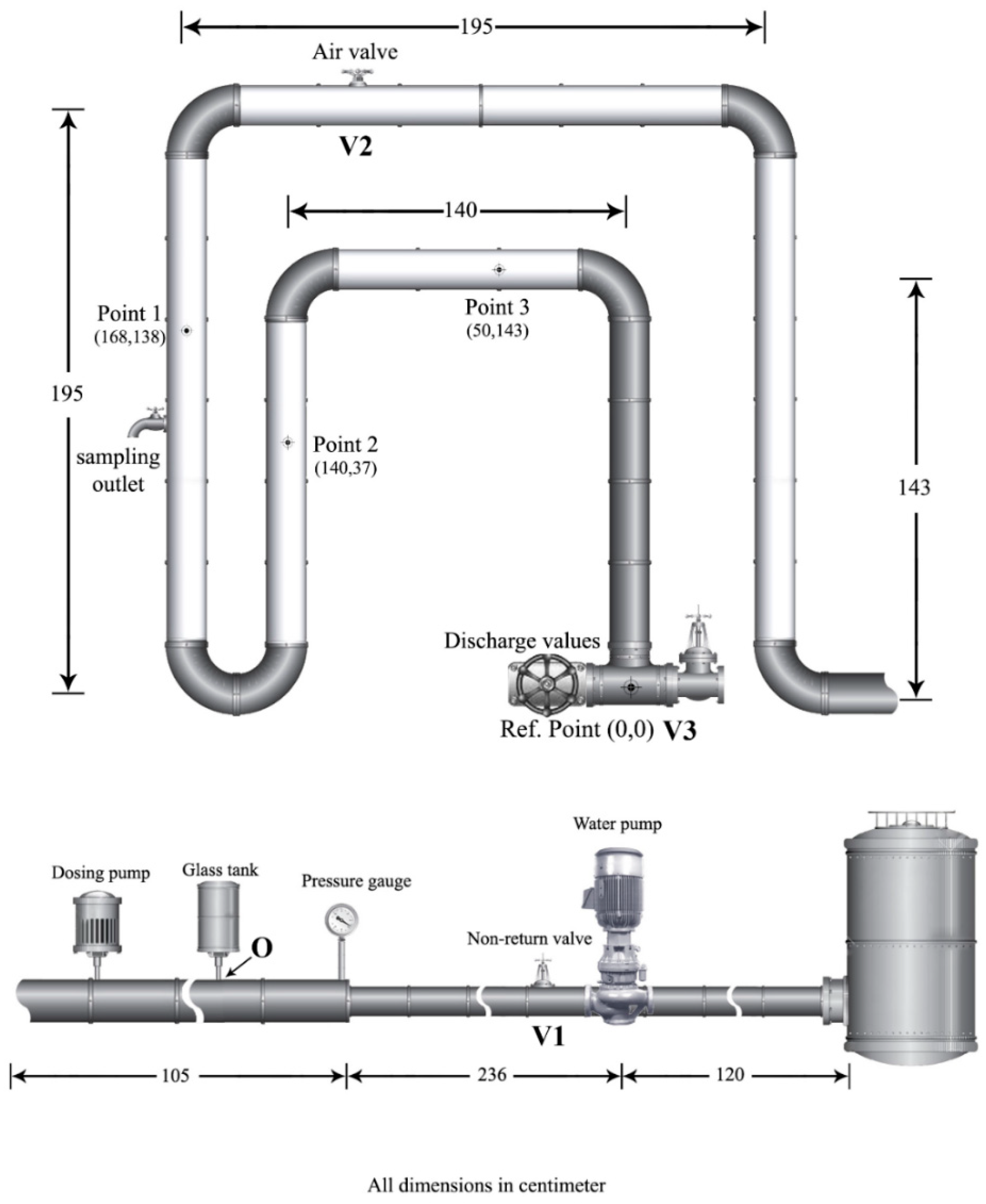
A pilot-scale experimental setup was constructed at the King Fahd University of Petroleum and Minerals (KFUPM) to investigate the potential of contaminant intrusion into a DWN under two main factors, namely, operation pressure variation and crack size. The study does not consider other factors related to contaminant reactivity or characteristics of soil media surrounding the pipeline. Thus, our experiment represents the worst-case scenario, which is often needed to undertake mitigation measures. The schematic diagram of the network is shown in Figure 1. The following sections describe the system general features and outline the procedure for the different experiments investigating the factors influencing the contaminant intrusion.

2.1. System Specifications/Description

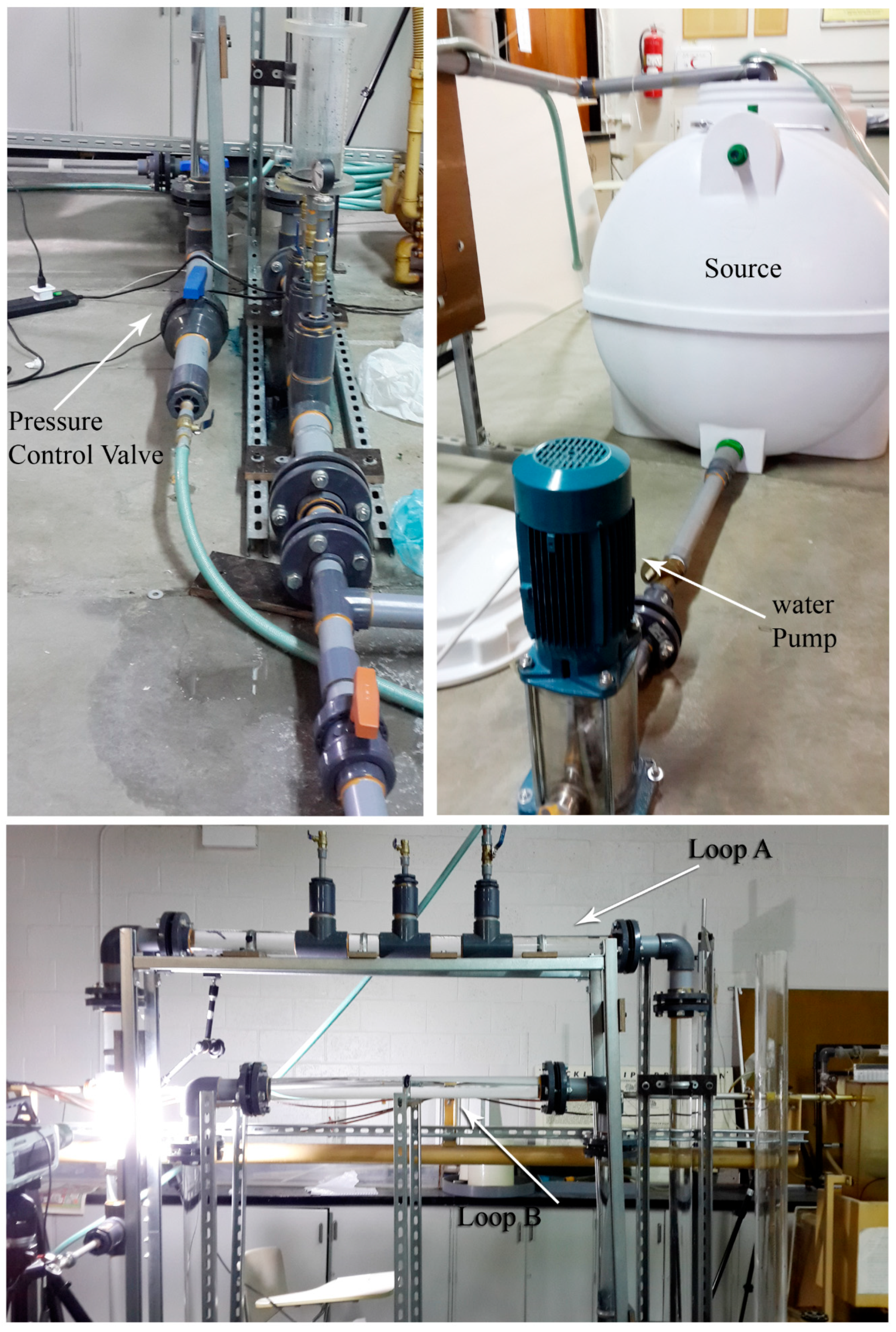
The experimental setup was designed to be used as either a circulating system (water goes back to the source tank) or an open pipe system (water goes directly to the drainage), as shown in Figure 1. The piping system contains two interconnected loops (A, and B) constructed from several 6-foot clear acrylic pipes (to enable the use of a high-speed camera) with an internal diameter of 6.35 cm (2.5 inches) and an external diameter of 7.62 cm (3 inches). The pipes were interconnected with several U-Shaped PVC joints. The dimensions of the external loop (A) are 195 cm (H) × 195 cm (L), while the internal loop (B) is 143 cm (H) × 140 cm (L). The two loops (A and B) are vertically mounted on a steel frame (Figure 2).

An air release valve (V2) was installed in the outer loop (A) to facilitate air removal from the pipes. Water was fed into the system from a 1000ℓ tank placed on the ground. The tank was connected with a 5.08 cm (2-inch) PVC pipe (P1) with a length of 120 cm that feeds the water into a water pump (WP). The pump generates the pressure required for the system to start the flow and was regulated by a non-return valve (V1).

Pressure was measured using a pressure gauge (PG); the tank was connected to the piping system through a control valve (V3) to control the pressure in the system, and a 2ℓ graded glass tank (GT) was filled with an inert food coloring (Foster Clark’s^TM Blue Food Color from Foster Clark Products Ltd., San Gwann, Malta) representing the contaminant. This inert contaminant has two characteristics: (1) it does not react with surrounding substances under the experimental conditions; and (2) it does not influence the motion of the water in the pilot setup. An optional dosing pump (DP) was placed after the GT. The GT and the DP gave the experiment operator the flexibility to simulate the cracks by introducing the contaminant either to naturally flow into the system at a low or negative pressure or to pressurize the contaminant through the system using the DP. A PHANTOM^TM v-Series high-speed camera was used to capture and track the contaminant flow through the acrylic pipes using Phantom Camera Control Software Version 2.6.749.0. Time measurements for all the experiments were done using a Fisherbrand^TM stopwatch.

2.2. Determination of the Minimum Time Required for the Contaminant to Initially Intrude the System

The experimental procedure at this phase included turning on the water pump and adjusting the flow pressure using V3 and PG to be set to different values (1, 2, 3, and 4-bars). Then a sudden shut down of the water pump was performed to create a low or negative pressure condition and simultaneously allowing contaminant intrusion through a 0.1-inch orifice (O) as seen in Figure 1. The orifice was used to control the size of the simulated crack. The pressure in the system was observed to decrease at the same time that a certain volume of water is pumped out of the system, filling up the GT (the contaminant container). The time was measured from the moment of turning off the water pump until the contaminant is introduced into the system. The experiment was then conducted at different operating pressures (1, 2, 3, and 4-bars), and each time, the minimum time required to start contaminant intrusion was measured. The experiment was repeated 3 times at each pressure, and the average times were recorded. The system was thoroughly flushed after each experiment to make sure that there is no remaining traces of the food coloring.

2.3. Determination of the Time Required for Full Contaminant Intrusion

A similar procedure as that used in the experiment explained in the previous section was applied to determine the time required for full contaminant absorption into the system. The time was calculated from the moment the water pump was turned off until full absorption of the contaminant into the system. Three different orifice openings—representing the crack size—were tested (0.1, 0.25, and 0.5 inch) under four different operating pressures (1, 2, 3, 4-bars).

2.4. Determination of Time Required for a Contaminant to Reach Selected Observation Points

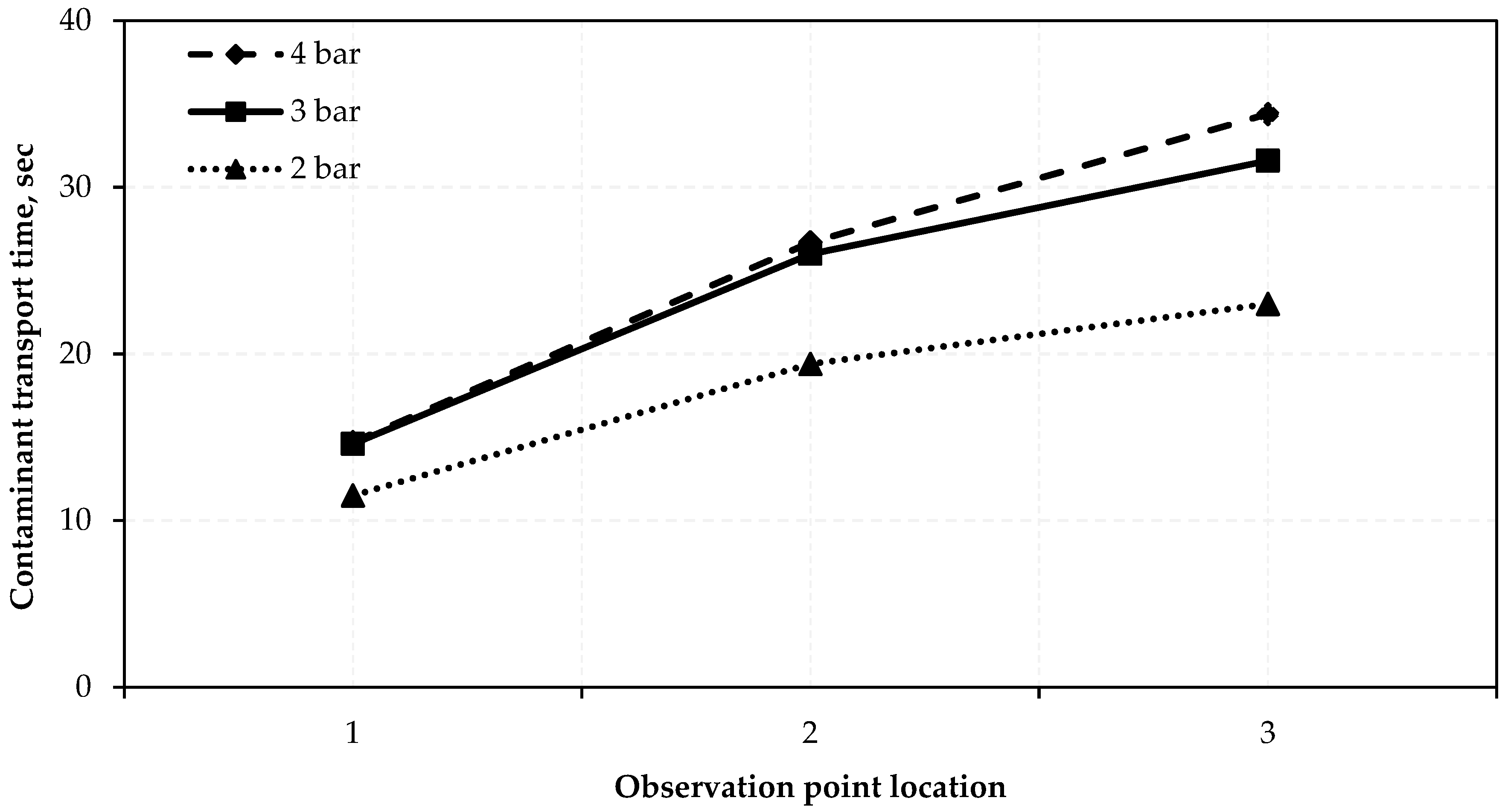
To evaluate the transport of the contaminant within the system, the time required for the contaminant to reach three specific observation points was measured. The three observation points (Point 1 {168, 138}, Point 2 {140, 37} and Point 3 {50, 143}) in the pipe system are shown in Figure 1. The procedure in this experiment included turning on the water pump and adjusting the flow pressure using V3 and PG to be set to different values (2, 3, and 4-bars). Then a sudden shut down of the water pump was performed to create a low or negative pressure condition and simultaneously allowing contaminant intrusion through a 0.1-inch orifice (O), the pump was instantly turned on after complete intrusion of the contaminant to measure the time required for the contaminant to be transported in the system. Time was measured from immediately after turning off the water pump until the instant the contaminant cloud reached a selected point in the pipes. The initial contaminant concentration in the tank (GT) was kept constant at 40 mL/L. The time measurement was repeated 3 times for each pressure, and the average times were recorded.

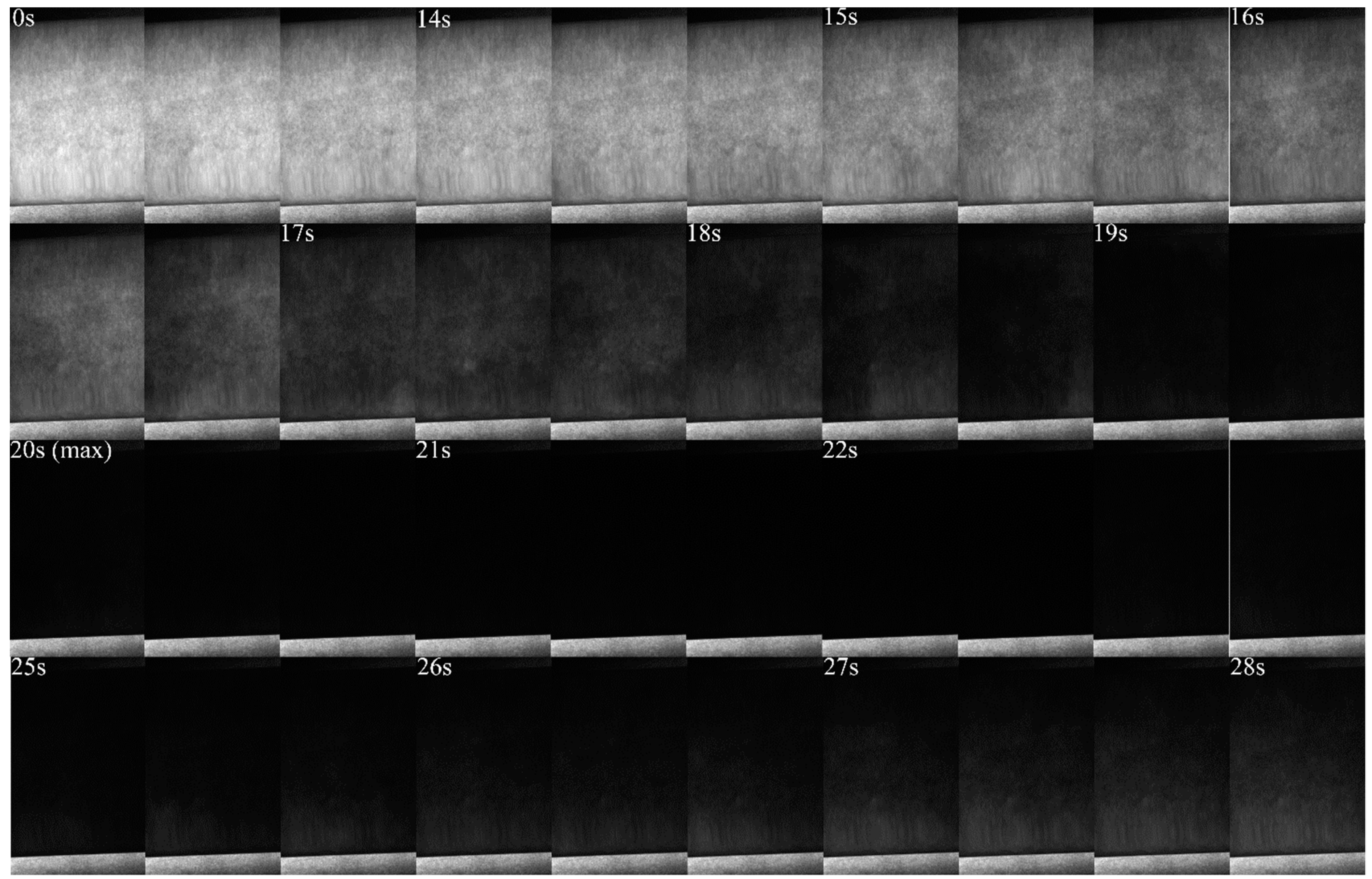
2.5. Visualizing Contaminant Flow Using a High-Speed Camera

The phenomenon of contaminant intrusion in the system was verified qualitatively using a high-speed camera. The camera was used to record this phenomenon that is not visually captured by the human eye, and it can also replay the action in slow motion. This was used as a validation of the time measurements taken in the contaminant transport experiment (Section 2.4). The camera was set to capture the contaminant intrusion into the system at three capture points (Point 1, 2, and 3). In each run, the camera and LED lights were set up at one of the observation points. Then, a dye (food coloring) was introduced to the system while the camera was recording through the acrylic pipes. After turning on the water pump, the contaminant began to progress throughout the system. When the contaminant reached the capture point and moved slightly past the capture point, the camera automatically ended the recording process.

2.6. Measuring Contaminant Concentration in the System

Measuring and monitoring the water quality in the DWN is critical to evaluate the associated risks to human health. The procedure for evaluating the contaminant concentration in the system included collecting 100 ml water samples using the sampling outlet (Figure 1) at different intervals (every 5 seconds for a duration of 35 seconds), under two operating pressures (2-bar and 3-bar) after the contaminant reached Point 1. Similar steps were then repeated after the contaminant reached Point 2 and Point 3. Sample collection did not affect the flow pressure as the sample outlet was left open throughout the experiment. Two steps were followed to determine the concentration of the contaminant (food coloring) in the system. The first step was to measure the absorption of each standard contaminant concentration (10, 20, 30, 40, and 50 mL/L) using an Ultraviolet-visible spectrophotometer (Shimadzu UV-2550) to create a calibration curve. Ultraviolet-visible spectrophotometry is a method that measures the absorption of a substance in the visible range of colored chemicals. This measurement of absorption was correlated to standard concentrations. The second step was to measure the absorption of the samples collected from the system and correlate the results to the calibration curve. Step 2 was repeated 3 times, and average measurements were recorded.

2.7. CFD Modeling

It is important to mention that CFD modeling is mainly useful to determine contaminant concentration at different locations of the DWN where sample collection is not possible. It was also used to verify experimental findings and to provide the flexibility of exploring different experimental setups and dimensions in future analysis.

COMSOL Multiphysics^® Modeling Software, (COMSOL, Burlington, MA, USA) is a finite element analysis, solver and simulation software used to solve various physics and engineering based applications. COMSOL Multiphysics 4.4 was used to model the flow of water and contaminant through the water network at different operating pressures and times. The experimental design was simulated using the COMSOL Desktop interface with the same pipe dimensions and structure as those used in the actual lab experiment.

A pseudo-time-dependent laminar flow model was considered throughout the simulation, which is described using the Navier-Stokes equations as:

$$\frac{\partial \rho }{\partial t}+\nabla .\left(\mathsf{\rho }\stackrel{\rightharpoonup }{u}\right)=0$$

(1)

$$\rho \frac{\partial \stackrel{\rightharpoonup }{u}}{\partial t}+\rho \left(\stackrel{\rightharpoonup }{u}.\nabla \right)\stackrel{\rightharpoonup }{u}=\nabla .\left[-P\stackrel{\rightharpoonup }{I}+\tau \right]+\stackrel{\rightharpoonup }{F}$$

(2)

where Equation (1) is the continuity equation that represents the conservation of mass, and Equation (2) is a vector equation that represents the conservation of momentum. $\rho$ is the fluid density (kg/m³); $\stackrel{\rightharpoonup }{u}$ is the velocity vector (m/s); P is the pressure (Pa); $\tau$ is the viscous stress tensor (Pa) (depends on the fluid dynamic viscosity); $\stackrel{\rightharpoonup }{F}$. is the volume force vector (N/m³); and $\stackrel{\rightharpoonup }{I}$ is the identity vector.

As temperature variations in the flow are negligible, the flow was assumed to be incompressible ($\rho$ is constant) and Equation (1) can be reduced to:

$$\rho \nabla .\stackrel{\rightharpoonup }{u}=0$$

(3)

To solve Equation (2), an initial guess close to the final solution is required; otherwise, the software will go through the process of solving fully transient problems, which requires a large amount of computational time. In this study, instead, we are using a pseudo time step approach to discretize the equation system and effectively transform a nonlinear iteration into a time step of size $\mathsf{\Delta }t$. No slip boundary condition was applied to the walls of the pipes.

The contaminant was simulated using a COMSOL Multi-physics transport of the diluted species interface where convection and diffusion are considered as transport mechanisms, which is governed by the mass balance equation:

$$\frac{\partial c}{\partial t}+\stackrel{\rightharpoonup }{u}.\nabla c=\nabla .\left(D\nabla c\right)$$

(4)

where c is the contaminant concentration (Mol/m³) and D is the diffusion coefficient (m²/s). The first term in Equation (4) represents the rate of contaminant accumulation, and the second term describes convective transport due to the fluid velocity. The term on the right-hand side accounts for contaminant diffusion transport, resulting from the interaction between the contaminant and the fluid. This equation assumes that the contaminant concentration is very small (diluted) compared to the solvent and that the mixture properties (viscosity, density) can be assumed to be the same as those of the solvent. The simulation was performed using 3162 element mesh (area ~9811 cm²) that contains 2010 triangular elements, 1152 quadrilateral elements, 690 edge elements, and 37 vertex elements.

3. Results

3.1. Minimum Time Required for a Contaminant to Initially Intrude the System

The results presented in Figure 3 show that there is a direct relationship between the operating pressure and the minimum time required for a contaminant to initially intrude the system. The results shown in Figure 3 include the average and error bars from the 3 repeated experiments for each operating pressure. It can be observed that the experiment shows good repeatability with only slight variations in the results obtained for each operating pressure. It should be noted that the minimum time required to start contaminant intrusion is affected by the accuracy of the experimental operator in opening the contaminant orifice simultaneously with turning off the water pump. As the orifice size is manually controlled through a valve, the orifice size could slightly change while conducting different trials of the experiment. Results show that the average minimum time required for initial contaminant intrusion at operating pressure of 2-bar is approximately 5.7 s. This time increases gradually to reach 10.3 s under operating pressure of 4-bar. This result indicates that when running the system at higher pressure, it will require more time for a contaminant to intrude the system. In addition, the results suggest that real-time safety measures should be implemented during the minimum time of intrusion if the system operating pressure is known.

3.2. Time Required for the Contaminant’s Full Intrusion

In this section, the direct relationship between operating pressure and the required time for full contaminant intrusion with respect to orifice size (representing a crack) will be discussed. Figure 4 shows that when pressure increases the contaminant requires more time to intrude the system. This is likely due to the increase in the water volume being pumped from the system into the contaminant container (GT) once the pump is turned off. For the 0.1-inch orifice size, the time required for a contaminant to fully intrude the system increases gradually with the increase of the operating pressure, starting from 24 s for 1-bar and reaching 42 s for 4-bar. The other two orifice sizes, 0.25 and 0.5 inches, had the same trend, except that it requires more time (+2.8 s on avg.) for the contaminant to fully intrude the system at an operating pressure 1-bar to 3-bar. However, with an operating pressure of 4 bar, the system exhibits a different behavior in which the time required for full contaminant intrusion decreases compared to 1, 2, and 3 bar pressures. This situation for operating pressure of 4-bars could be attributed to a larger head created by the water accumulating into the contaminant container (GT) when the water pump is turned off. This larger head could expedite the contaminant intrusion through the larger orifice sizes.

It was interesting to observe that when the system was running at its normal operating pressure, the contaminant did not enter the network, due to the high pressure maintained in the system. Additionally, it was observed that when there was no consumption or flow going out of the system, even with the pump shutdown, the contaminant did not enter the system. Overall the experimental results show that once the water pump is turned off the water flows out of the system through the orifice (representing a crack) and into the contaminant container. Depending on the operating pressure and the network design, the water and contaminant mixture is then absorbed back into the system. In the next section, the time required for the contaminant to be observed in the system is calculated.

3.3. Time Required for a Contaminant to Reach Selected Observation Points

This section evaluates the propagation of the intruded contaminant in the system by studying the time required for the contaminant cloud to reach selected observation points simulating consumer outlets. For 2-bar operating pressure, the time required for the contaminant to reach point 1 is 11 s, while it takes 14 and 15 s under operating pressures of 3-bar and 4-bar respectively. Since points 2 and 3 are further from point 1, the contaminant requires more time to reach these points. Since the control of the pressure in the pilot system relies on the partial closure of the control valve (V3), it follows that this also changes the flow in the system. The transport of the contaminant in the system relies mainly on the flow velocity in the system, which for the set pressures of 2, 3, and 4 bars was 0.056, 0.034, and 0.014 m/s, respectively. This explains the observation shown in Figure 5 that for high pressures the time required for a contaminant to move from the source until reaching locations 1, 2, and 3 is significantly longer than that under low pressures (for instance, at point 3: it requires 23 s for 2-bar 35 s for 4-bar). This can be attributed to the decrease in flow velocity associated with the increase in pressure due to valve closure. This indicates that locations with higher water consumption at the DWN will be more exposed to the contaminant.

3.4. Qualitative Assessment of the Contaminant Intrusion Using High-Speed Camera

The qualitative results were obtained using a high-speed camera. The camera was used as a validation of the time measurements taken at the three observation points (Point 1, 2, and 3). The results in Figure 6 show the consistency between the time measurements and the contaminant concentration (40 mL/L) captured by the camera at a system operating pressure of 3-bars. The picture shows a zero concentration at the beginning of the experiment; then the contaminant started to gradually appear in the camera (time = 14 sec). Then at 20 sec, the maximum concentration occurred and can be seen clearly in Figure 6. As the system is not circulating the water, the contaminant began to diminish and was washed out by the system. The experiment was repeated for the three operating pressures (2, 3, and 4-bars), and the results trend was similar for all system operating pressures. The differences in the time required for the contaminant to reach the observation points 1, 2, and 3 under the different operating pressure matches the differences observed in Figure 5 (contaminant transport time increases with the increase in pressure).

3.5. CFD Modelling Results

The experimental results were verified using CFD analysis. The experimental results for contaminant concentrations were obtained by recording concentrations in the samples’ collected at the pilot network’s sampling outlet using the UV spectrophotometer. The results in Figure 7 show a similar trend for both experimental and CFD concentrations for the samples taken from the sampling outlet. The contaminant was not observed in the DWN until 13 s from turning on the pump; this was true for both experimental and CFD results. The concentrations started to increase with time to reach 4 mL/L and 3 mL/L for experimental and CFD results, respectively. Then, the concentrations decreased slightly to 2.2 mL/L and 1 mL/L at 38 s for experimental and CFD results, respectively. Overall, the concentration recorded using the UV spectrophotometer displays higher concentrations between the times from 20–40 s.

Modeling of the contaminant’s dispersion in the system is displayed in Figure 8 for an initial contaminant dose of 40 mL/L and 2 bars of operating pressure. The arrow in Figure 8 points to the contaminant concentration at point 3 (50, 143) at 24, 28, and 30 s, where the high-speed camera was used to take shots at this location. The simulation shows a similar trend, as shown in Figure 6, which indicates that the contaminant cloud progresses faster in the experimental setup than in the CFD modeling, which is also verified by the results in Figure 7. This could be attributed to uncertainty in pressure measurements, the manual control on orifice size, and/or the manual sample collection from the system to perform the contaminant concentration tests [32].

4. Discussion

Simulation-based investigation of contaminant intrusion into drinking water distribution systems was used in previous studies [2,33,34,35]. In this study, the use of CFD modeling combined with the high-speed camera proved to be a useful approach for validating the quantitative experimental results. The high-speed camera recorded a very detailed video about the contaminant transport throughout the system. This method was useful to qualitatively investigate the contaminant intrusion as adopted by similar studies, such as Fox et al. 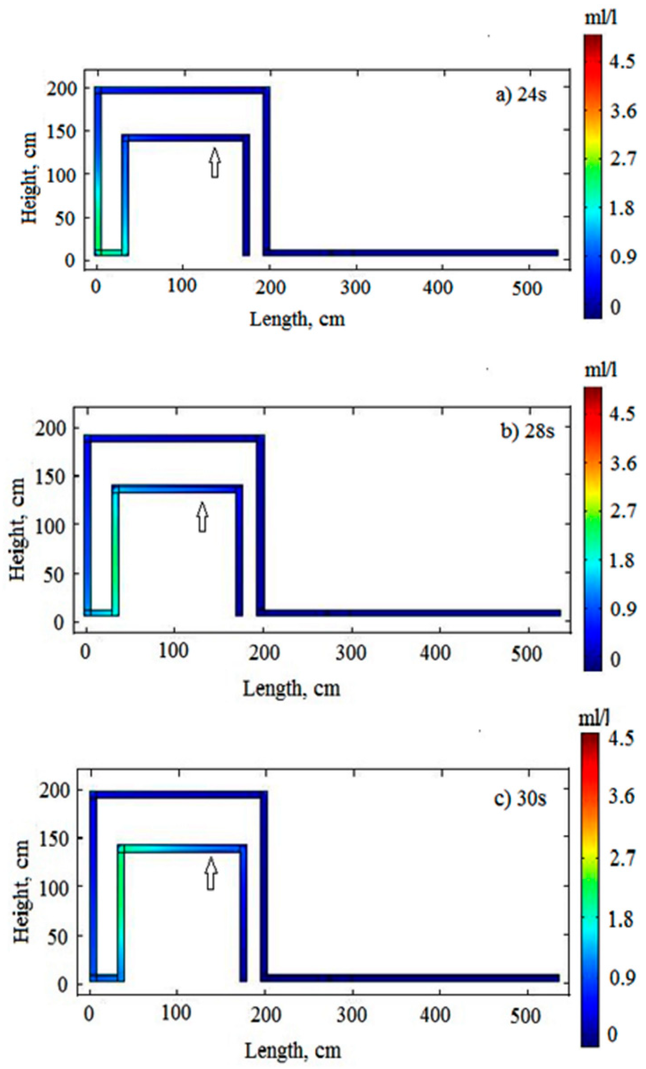2016 [28]. In this study, it was found that there is consistency between the time and concentration measurements captured by the camera and the corresponding experimental sampling measurements. Similarly, the use of CFD modeling supported the quantitative and qualitative investigation by providing additional simulated information on the progression of the contaminant. 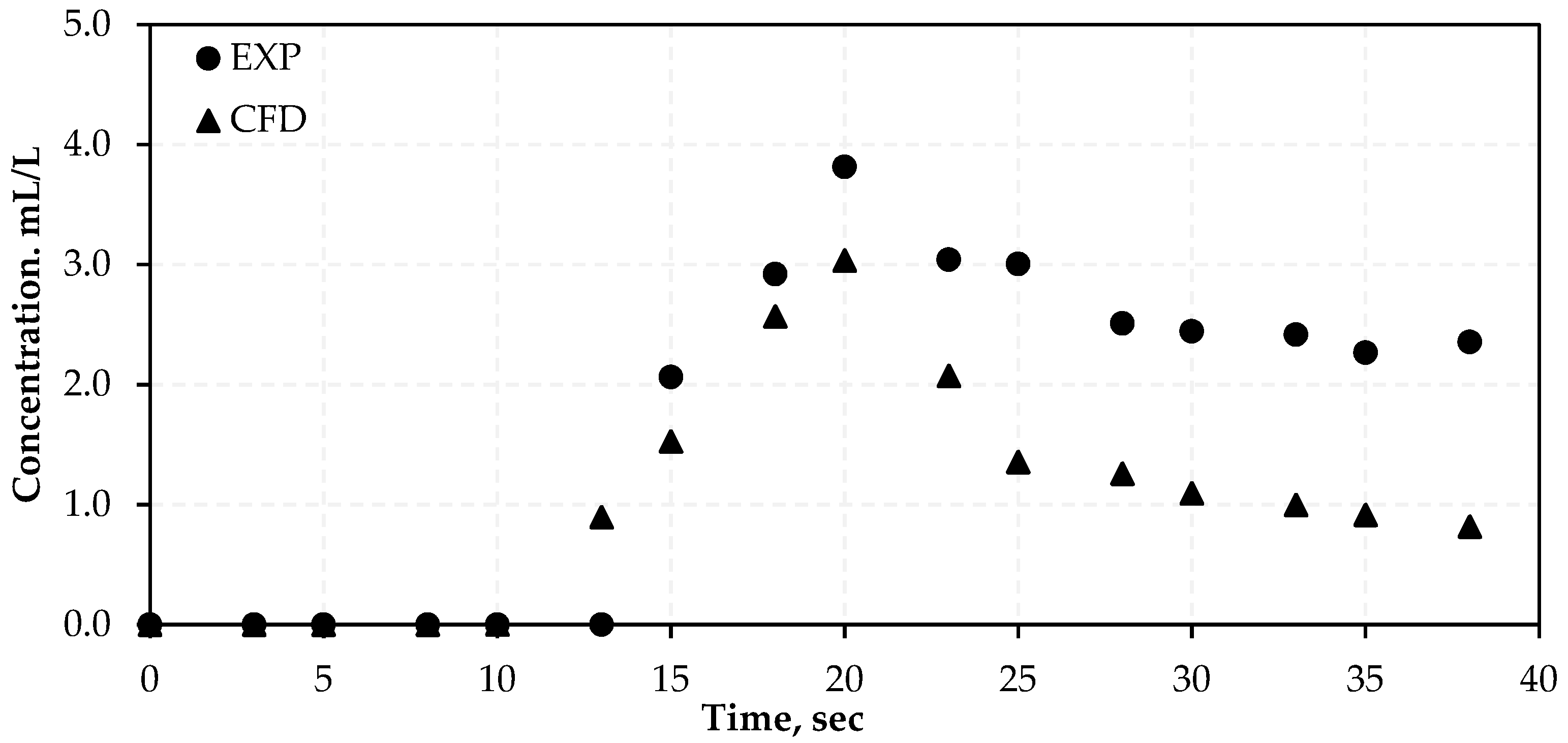Previous researchers have used CFD modeling to help increase the understanding of factors affecting the contaminant intrusion process, particularly considering a wider range of factors to study the associated risk and health impact [35,36,37]. In general, it was observed that the quantitative experiment produced higher contaminant concentration than that from the CFD modeling. Such differences between experimental and modeling results were observed by other researchers such as Fox et al. 2016 [28].

In theory, the process for contaminant intrusion following a low or negative pressure starts with an immediate ingress into the system through pipe cracks [23,26,35]. Nevertheless, it was quite interesting to observe, in this study, that the pipe water is first pumped out of the system into the contaminant tank (which represents soil surrounding a real DWN), mixes with the contaminant and then the solution is absorbed back into the DWN. By not considering the impact of soil media on contaminant intrusion, the experiment in this study represents the worst-case scenario, which is often needed to undertake mitigation measures. There is an indication that the risk of contaminant intrusion through cracks in pipes buried under the ground is insignificant if water pumps were shut down only for a few seconds, which was mentioned in previous studies [24]. Results also show that the minimum time required for the contaminant to intrude into the system is not affected by how long the system was running before the power shutdown. This means that even in the case of frequent power shutdowns, the probability of a contaminant intrusion into the DWN is very small as long as the system has enough time to stabilize its pressure after each shutdown. The only factor affecting the time required for the contaminant to intrude the system is the operating pressure. As the results point out that when running the system at high pressure it will require more time for a contaminant to intrude the system, real-time safety measures can be implemented before the contaminant intrudes the system.

The time required for the contaminant to move from the source until reaching locations 1, 2, and 3 was significantly longer during higher pressure than that under lower operating pressures. This was attributed to the decrease in flow velocity associated with the increase in pressure due to valve closure. This means that the progress of the contaminant within the distribution network depends mainly on the velocity of flow, making areas with higher water consumption more exposed to the contaminant. This result could help water system operators identify the relevant management strategies that can be adopted to mitigate the impact of contaminant intrusion for zones with higher water consumption. These strategies are contaminant-specific, site-specific, jurisdiction-specific, and limited by the availability of technology and resources [19]. Contaminant intrusion management is also related to general water system operation, particularly with regards to system monitoring and control (e.g., system shutdown). Some common mitigation measures include maintaining residual disinfectant, maintaining positive pressure, system flushing, etc.

5. Conclusions

Experimental work and CFD analysis were performed to investigate contaminant progression in a DWN. Scenarios of low pressures due to sudden power shutdowns were investigated, and the contaminant intrusion into the system was measured. It was shown that under low transient pressure conditions the intrusion of an external contaminant through the pipe crack (orifice) occurred. In general, the results from the CFD modeling, experimental measurements, and qualitative assessment using a high-speed camera were consistent, with only slight differences. Results concluded that the time required for the contaminant to intrude into the system is not affected by how long the system was running before the power shutdown, nor was it influenced by the frequency of shutdown as long as the system has enough time to stabilize its pressure after each shutdown. Furthermore, the progress of the contaminant within the distribution network was shown to mainly depend on the velocity of flow, making areas with higher water consumption more exposed to the contaminant. This result could help water system operators identify the relevant management strategies that can be adopted to mitigate the impact of contaminant intrusion for zones with higher water consumption.

The use of an inert contaminant in this study was necessary to avoid overlapping the studied factors with those related to the contaminant reactivity. It is recommended that future studies should investigate the impact of using reacting contaminants simulating real-world situations on the rate and concentration of the intruded contaminant. This study could help form a solid foundation for further studies to extensively investigate the risk associated with contaminant intrusion into drinking water systems. This can be achieved by including other factors (internal, external, and environmental factors influencing drinking water supply) that were blocked in this study to limit the study bias and associated error. In addition, an extension of this study could be through introducing different types of contaminants and including their respective risk of illness due to exposure in quantifying the health impact of contaminant intrusion in a DWN.