Effect of the Area Contraction Ratio on the Hydraulic Characteristics of the Toothed Internal Energy Dissipaters


1
College of Water Resources and Engineering, Taiyuan University of Technology, Taiyuan 030024, China
2
Water conservancy engineering design Ltd. of Shanxi Qian Cheng, Taiyuan 030024, China
*
Author to whom correspondence should be addressed.
Water 2019, 11(7), 1406; https://doi.org/10.3390/w11071406
Submission received: 16 May 2019
/
Revised: 30 June 2019
/
Accepted: 3 July 2019
/
Published: 9 July 2019
(This article belongs to the Special Issue Environmental Hydraulics Research)
Abstract
:Toothed internal energy dissipaters (TIED) are a new type of internal energy dissipaters, which combines the internal energy dissipaters of sudden reduction and sudden enlargement forms with the open-flow energy dissipation together. In order to provide a design basis for an optimized body type of the TIED, the effect of the area contraction ratio (ε) on the hydraulic characteristics, including over-current capability, energy dissipation rate, time-averaged pressure, pulsating pressure, time-averaged velocity, and pulsating velocity, were studied using the methods of a physical model test and theoretical analysis. The main results are as follows. The over-current capability mainly depends on ε, and the larger ε is, the larger the flow coefficient is. The energy dissipation rate is proportional to the quadratic of Re and inversely proportional to ε. The changes of the time-averaged pressure coefficients under each flow are similar along the test pipe, and the differences of the time-averaged pressure coefficient between the inlet of the TIED and the outlet of the TIED decrease with the increase of ε. The peaks of the pulsating pressure coefficient appear at 1.3 D after the TIED and are inversely proportional to ε. When the flow is 18 l/s and ε increases from 0.375 to 0.625, the maximum of time-averaged velocity coefficient on the line of Z/D = 0.42 reduces from 2.53 to 1.17, and that on the line of Z/D = 0 decreases from 2.99 to 1.74. The maximum values of pulsating velocity on the line of Z/D = 0.42 appear at 1.57D and those of Z/D = 0 appear at 2.72D, when the flow is 18 l/s. The maximum values of pulsating velocity decrease with the increase of ε. Finally, two empirical expressions, related to the flow coefficient and energy loss coefficient, are separately presented.
1. Introduction
The internal energy dissipater effectively reduces the downstream flow speed, smoothly connects the downstream flow, and avoids the erosion of the river channel by a traditional energy dissipater in a water conservancy project with high water head and high flow. This is because it converts the large area effect of high-speed water flow into a local energy dissipation effect. The most common form of internal energy dissipation is the energy dissipaters with sudden reduction and sudden enlargement. The energy dissipaters with the sudden reduction and sudden enlargement forms are a pressure energy dissipation method that uses the sectional contraction water flow to adjust and dissipate excess energy [1], and its hydraulic characteristics are mainly affected by the geometric size of energy dissipaters.
The common energy dissipaters with sudden reduction and sudden enlargement forms were divided into orifice plates and plugs (thick plates) according to their thickness along the flow direction [2], and many researchers investigated their hydraulic characteristics and influencing factors. It was found that the contraction ratio was an important factor affecting the hydraulic characteristics of the plug [3], and the shape and thickness of the plug also had a great influence on the flow characteristics [4]. The affecting factors of head loss coefficient for orifice plate, such as relative thickness, area contraction ratio (ε), and Reynolds (Re), were studied by Wu [5], who proved that relative thickness and ε of orifice plate were important geometric factors affecting the head loss coefficient. Some researchers mainly focused on the energy dissipation rate and over-current capability of internal energy dissipaters with different body types and area contraction ratios. The energy dissipation ratios of single and two-stage plug energy dissipaters were obtained by the combination of a physical model and numerical simulation [6]. The energy dissipation ratio of a plug, with the combination of the vertical jet, straight curved hole plugs, and horizontal hole plugs was designed and analyzed [7]. The change of pressure was also one of the hydraulic characteristics concerned. The study concluded that the pressure pulsation decreased with the reduced cross-sectional area for the orifices plate [8]. The numerical simulation of pressure field for the thin and thick plates was conducted, and the change law of the sectional pressure drop was analyzed [9]. The distribution of wall pressure coefficient for the orifice dissipaters was discussed [10]. The distribution characteristics of mean flow velocity and pulsating velocity for the orifice plate or the plug were obtained by the simulated or measured flow fields [11,12]. Meantime, scholars have also studied the cavitation characteristics of orifice plates and plugs. The cavitation characteristics of orifice plates and plugs, the cavitation mechanism, and influencing factors of orifice dissipaters were studied by Ai [13]. Additionally, cavitation numbers decreased with the increase of ε for the internal energy dissipaters with the sudden enlargement and reduction forms in the work of Zhou [14] and Zhang [15]. To sum up, the area contraction ratio (ε) of internal energy dissipation with sudden enlargement and reduction was an important geometric factor to decide its hydraulic characteristics.
On the basis of previous studies, new internal energy dissipaters called toothed internal energy dissipaters (TIED) were proposed by our research team [16], which combines the internal energy dissipaters of the sudden reduction forms and sudden enlargement with the open-flow energy dissipation. The flow characters affecting the body factors of the TIED were discussed, and the reasonable body factors of the TIED were preliminary optimized [17,18,19]. In previous works, the body shape of internal energy dissipater was the key to analyze the variation of the hydraulic characteristics, and the area contraction ratio was the most critical body geometry parameter influencing the hydraulic characteristic of the TIED.
In order to study the effect of the area contraction ratio (ε) on the hydraulic characteristics of TIED, it is necessary to confirm the length, height, and angle of piers. Some researchers mainly focused on the length and height of the plug and TIED. The effect of the length of the plug [20] and piers [21] on the head loss coefficient was analyzed via numerical simulation. It was found that the head loss coefficient decreased sharply and then increased with the increase of their length, and its turning point was a length of 0.5D. When their length increased to 0.9D, the local head loss tended to be stable. The effect of the pier’s height on the hydraulic characteristics of the toothed internal energy dissipate (TIED) was studied via a physical model test [22]. The results showed that the energy dissipating effect was better when the height of the piers (h) was no greater than 0.25D, and the flow coefficient was larger when the height of piers (h) was equal to 0.25D. According to the results, the length and height of piers was initially chosen to be 13.5 cm (0.9D) and 3.75 cm (0.25D), respectively.
In this paper, five different types of the TIED with four toothed piers (the length of each toothed piers is 0.9D), which have different area contraction ratios (ε), were designed and used to experimentally study the effect of the area contraction ratio (ε) on hydraulic characteristics.
2. Model Experiment
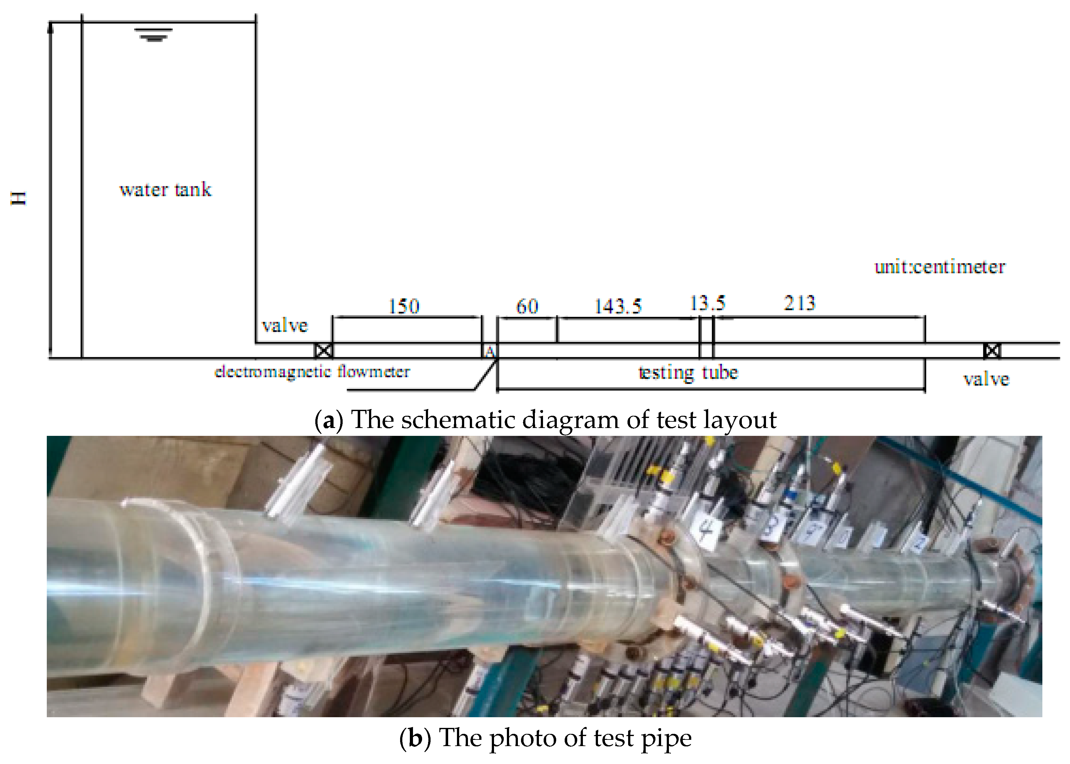
The test device consists of a flat water tank, a pipeline, an electromagnetic flow meter, a test section, and a valve. The test pipe is made of organic glass to observe the flow regime easily. The inner diameter (D) of the test pipe is 15 cm, and its total length is 370 cm. Figure 1 shows the layout of the test device.
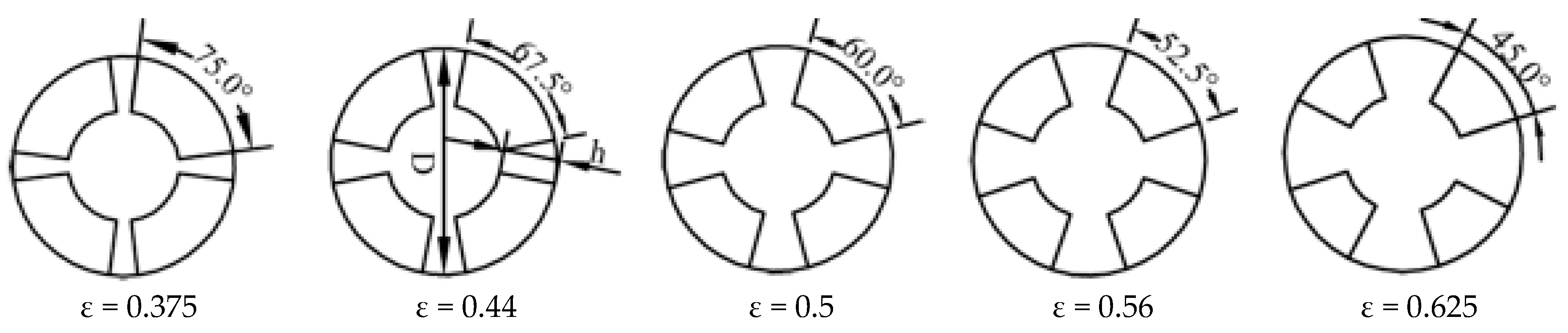
The TIED is located 143.5 cm away from the inlet of the test pipe, and its length (L) is 13.5 cm. For the TIED, the number of the piers (n) is 4, and the height of the piers (h) is 3.75 cm. The area contraction ratio (ε) can be defined as: . In equation, A0 is the cross-sectional area of TIED, A is the cross-sectional area of test pipe, and θ is the angle of the piers. In order to study the effect of area contraction ratio (ε) on hydraulic characteristics of the TIED, five types of TIED were experimentally studied via the physical model. The cross-sectional areas of the TIED are displayed in Figure 2.
During the test, the upstream head (H) was kept constant, the flow was constant in the test pipe, the indoor temperature was 20 °C, and the range of flow was between 18 l/s and 42 l/s. In order to analyze the same flow condition, the flow of each group was about 6 l/s increased sequentially, and the flow measurement error of each experimental flow group was ±0.2 l/s.
The flow (Q) through the test pipe and the transient pressure () along the bottom of the test pipe were measured for each test group. The center point at the inlet of the TIED is the origin of the coordinate, the direction of water flow is positive for the X axis, and the direction for vertical upwards is the positive Z axis. Q was measured using an intelligent electromagnetic flow meter, and its measured accuracy was ±0.5%.
was measured with a digital pressure sensor, and its measured accuracy was 0.1%, and its measuring frequency 100 HZ. Figure 3a shows the relative position of the pressure measuring points.
When Q was 18 l/s, the transient flow velocity (u) was measured by the DOP3010 flow velocity meter for different ε. The sampling frequency of the DOP3010 flow meter was 1MHz and its resolution was 0.01 mm. The angle between the measuring probe of u and the pipe wall was 70°, and their gap was filled with coupling medium to make the measurement of u more precise. Taking the measuring point of 1* as an example, it is possible to obtain the value of u for measuring points at intervals of 1 cm on the line of a. Z/D = 0 is at the central axis of the test pipe and Z/D = 0.42 is 1.2 cm away from the upper side of test pipe. The measured value of u is stable in the position of Z/D = 0.42 and Z/D = 0 for every measuring point. The relative position of the measuring point is shown in Figure 3b.
3. Analysis of the Flow Characteristics Affected by the Area Contraction Ratio
3.1. Over-Current Capability
The flow coefficient (μc) reflects the over-current capability of the test pipe, written as:
where is the head loss between the fifth and fourteenth measuring point.
is calculated by the following equation:
where and are the position head for the measuring points of 14 and 5, respectively, and the position head of is equal to that of ; and are the time-averaged pressure for the measuring points of 14 and 5, respectively; and are the average flow velocity for the measuring points of 14 and 5, respectively, and their value are equal to ; is the averaged velocity of the test pipe; is the head loss between the front and back of TIED; ξ is the head loss coefficient, and the sum of the resistance coefficient () along the pipe and the local head loss coefficient ().
Combining Equations (1) and (2) together, we can obtain:
The influencing factors of are the flow regime and the roughness of the pipe wall, and the roughness of the pipe wall is affected by the geometric parameters of the TIED. When the water flow is laminar, is only affected by Re. When the water flow is turbulent and in the transition zone, is determined by the roughness of the pipe wall and Re. When the water flow is turbulent in the square zone of resistance, is determined by the roughness of the pipe wall and not affected by Re. When Re is between 1.5 × 10⁵ and 3.5 × 10⁵, the water flow is located in the square area of turbulent resistance, is determined by the body type of the TIED, the wall roughness of the TIED, and the wall roughness of the testing pipe.
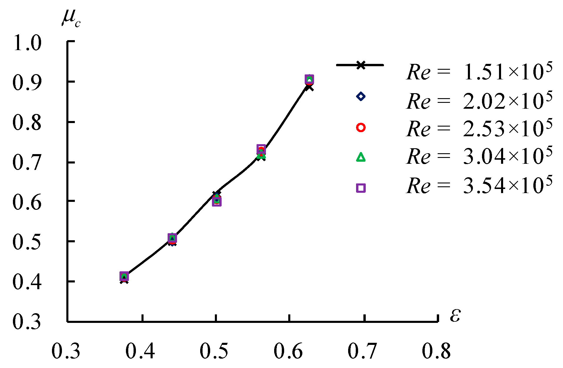
Figure 4 shows the change of the flow coefficients () with ε for different Re. is little affected by Re and its relative errors are within 2% for the same ε when Re is between 1.5 × 10⁵ and 3.5 × 10⁵. For the same Re, increases from 0.4 to 0.9 with the increase of ε, so ε is the main influencing factor of over-current capability.
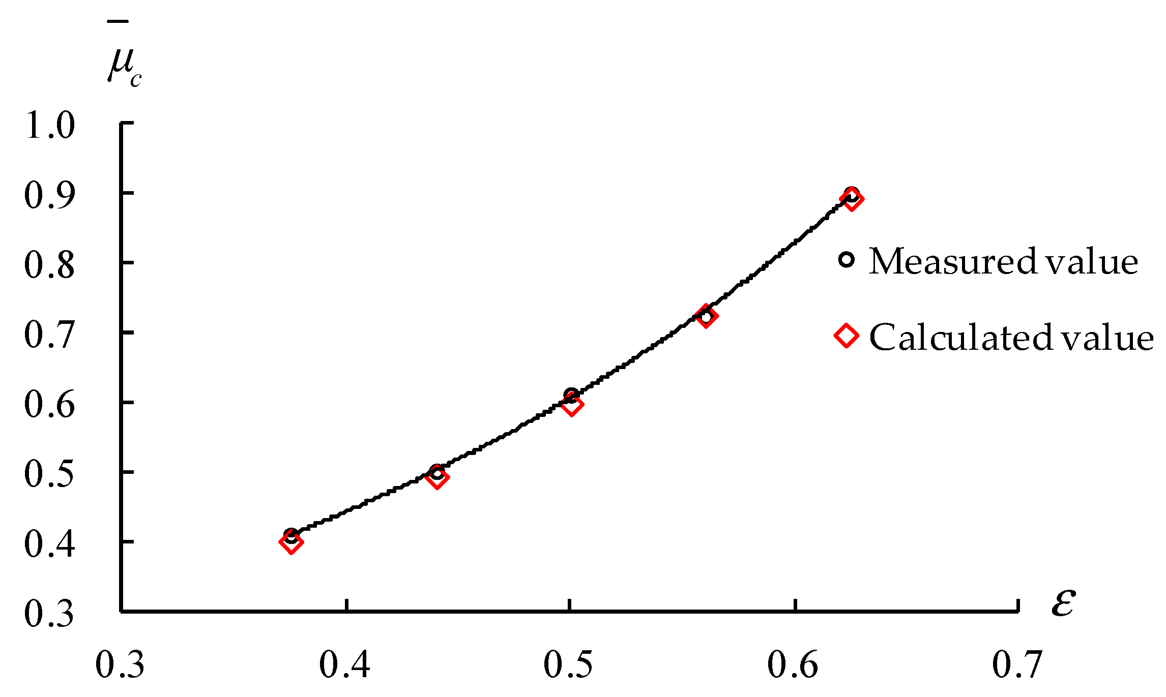
In order to eliminate the error of caused by the Re in the experiment, the averaged value () of for different ε is acquired in the testing flow range, and the relationship between and ε is presented in Figure 5. It indicates that increases with the addition of ε, and the empirical formula of is presented as:
The calculated values of obtained by Equation (4) and the measured values of are shown in Figure 5. Comparing the calculated values with the measured values for the same ε, their errors are smaller than 5% and within the range of allowable error. Therefore, Equation (4) can calculate the flow coefficient of the TIED in the testing flow range.
3.2. Energy Dissipation Rate
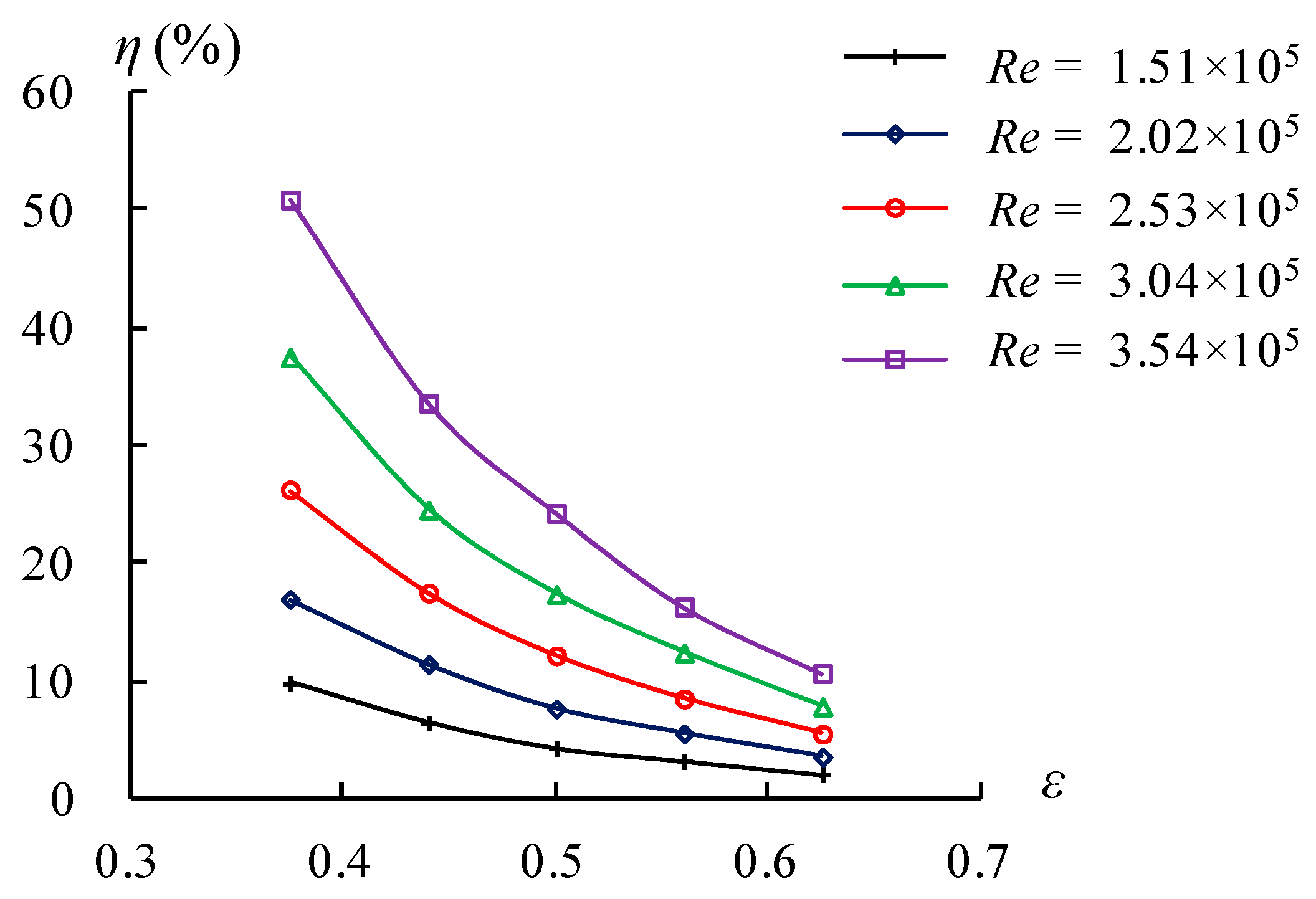
The energy dissipation rate (η) can represent the energy dissipation effect of the TIED. The higher the energy dissipation rate, the better the energy dissipation effect. It can be expressed as:
where is the head loss between the front and back of TIED, H is the total test head, ξ is the head loss coefficient, and v is the average velocity of test pipe.
Figure 6 shows the variation trend of η with ε in the condition of different Re. η increases with Re for the same ε and decreases exponentially with ε for the same Re.
Because of the constant total head in the test, Equation (6) can be transformed as follows, aiming to analyze the change of η:
In Equation (6), when ε is constant; ξ, g, A, and H are constant and η is proportional to the square of Q; when Q is constant, η is proportional to ε. Therefore, the value of η can be calculated by ξ in the case of a known Q.
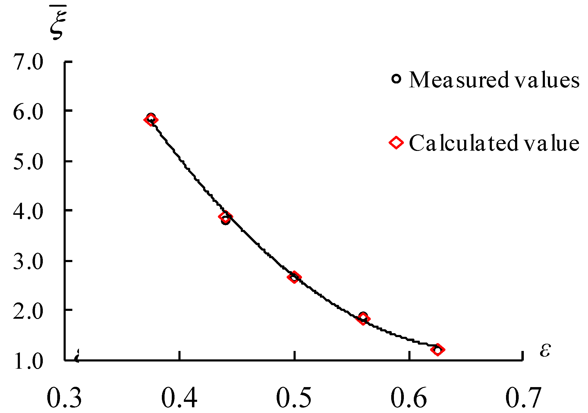
In order to eliminate the influence of Re on ξ, the average value () is obtained by taking an average of ξ in the testing flow range, and the change of with the increase of ε is shown in Figure 7. decreases from 5.9 to 1.2 when ε is between 0.375 and 0.625. The empirical formula of ξ can be expressed as follows:
The calculated values of ξ are obtained by Equation (7), and the measured values of ξ are obtained with the help of the model test. Both of them are presented in Figure 7. Comparing the calculated values of ξ with the measured values, the errors are less than 5%. Thus, this formula can calculate ξ for the TIED in the testing flow range. Moreover, it can obtain η to substitute ξ into Equation (6) in a certain flow.
3.3. The Variation of the Time-Averaged Pressure along the Test Pipe
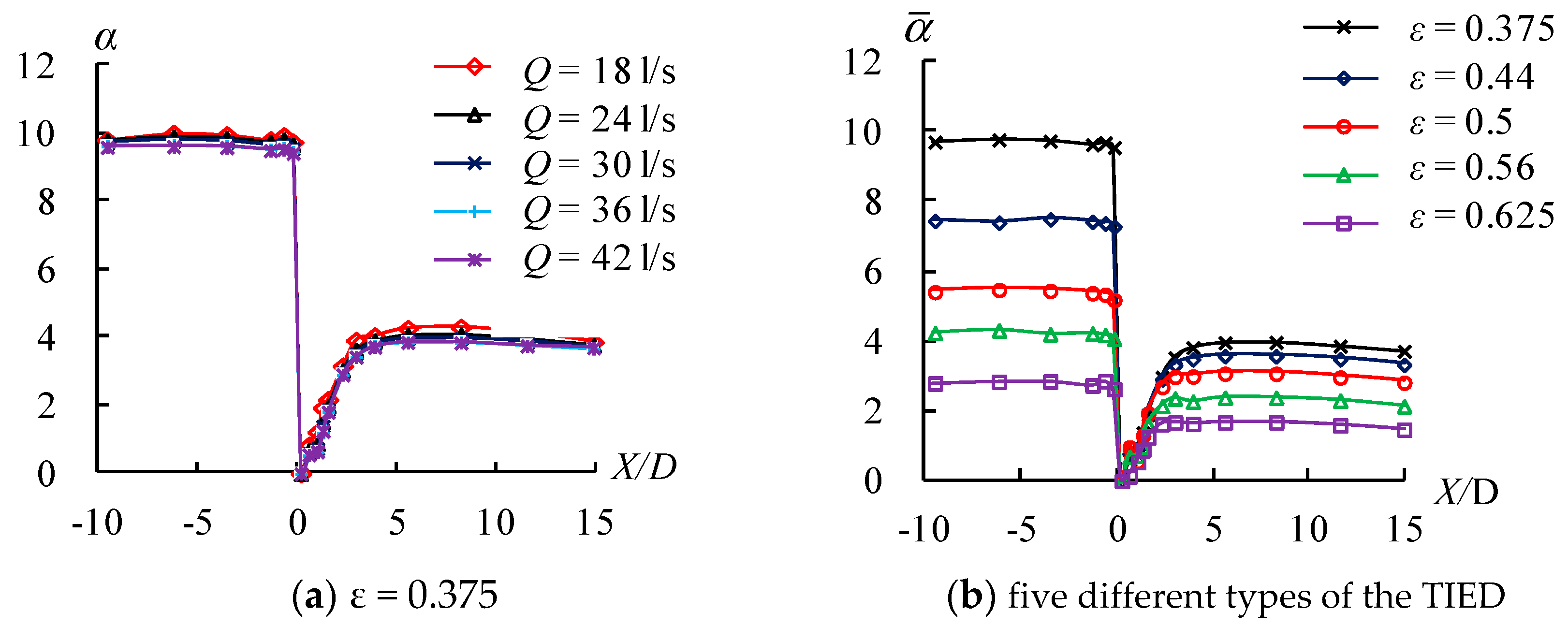
When Q increases in the pipeline, Re becomes larger, the frictional head loss and local head loss also become greater, and the reduced amplitude of the time-averaged pressure () decreases sharply along the test pipe. The time-averaged pressure coefficient (α) is introduced to express better, established as:
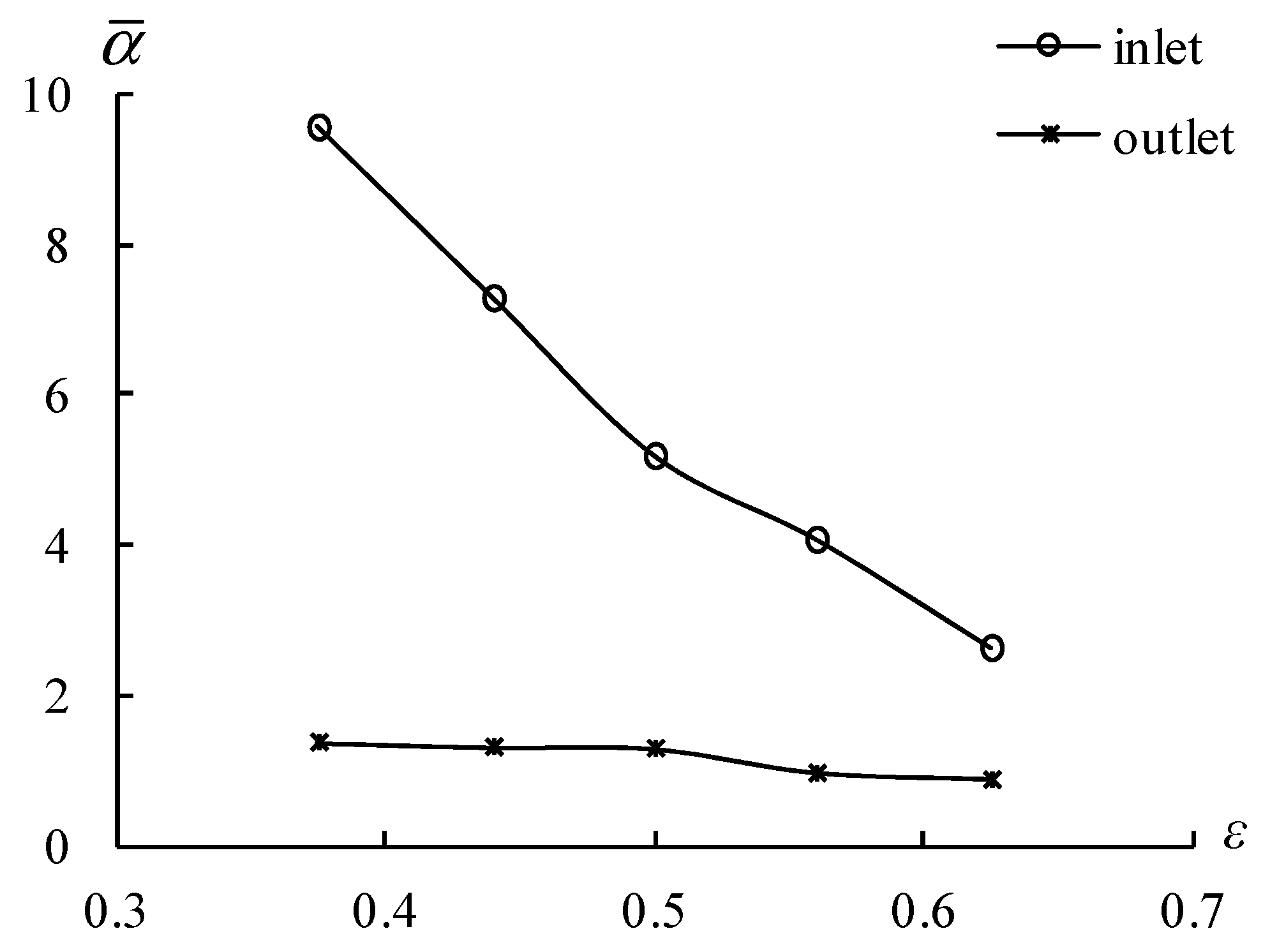
where is the time-averaged pressure for each measuring point; is the smallest value of the time average pressure among the measuring points along the test pipe; and its position pressure in the test is at 0.2D. Figure 8a shows the change of α along the test pipe. It can be seen that the time-averaged pressure coefficients are less affected by Q and have similar change trends along the test pipe. The reason is that the difference of α between the two measured points is equal to the head loss coefficient, and the effect of Re on the value of α can be neglected, and it was only affected by the energy dissipater. In order to reduce the error caused by the changes of Re, the average value () is obtained to study α better in the range of Q. The relationship between and ε is shown in Figure 8b, and the changes of with the increase of ε for the inlet or outlet of the TIED are presented in Figure 9.
As shown in Figure 8 and Figure 9, α drop sharply at the inlet of the TIED, then gradually increases and tends to remain nearly constant in the place of 4D after the inlet of the TIED. The reason is that the sudden changes of the flow velocity, caused by the sudden change of the flow cross-section through the TIED, lead to changes of α. For different types of TIED, α decreases from 9.8 to 2.8 before the inlet of the TIED and falls from 3.9 to 1.6 after the outlet of the TIED with the increase of ε from 0.375 to 0.46, and the minimum of α along the test pipe increases with the increase of ε. For different types of the TIED, in the outlet and inlet of the TIED both decrease with the increase of ε, and their differences drop from 8.2 to 1.8 when ε grows from 0.375 to 0.625. The change of α within and near the TIED is mainly due to the increase of the head loss coefficient, which is caused by the change of cross-sectional area.
When Q is constant, the smaller ε is, the larger in the front of the TIED is. Thus, the larger enough value of should be provided. Additionally, the value of is constant when Q is constant. Therefore, the value of will be negative with the decrease of ε. When ε is constant, is constant. The larger Q is, the smaller becomes, so the value of will be negative with the increase of Q. In the testing range flow, when the flow is about 42 l/s and ε is equal to 0.375 and 0.46, the value of is negative. The air will enter the pipe when the value of time-averaged pressure is negative, and then cavitations are likely where the flow velocity becomes small.
3.4. Variation of Pulsating Pressure
The size of the pulsating pressure can be represented by the root mean square of the pulsating pressure (σ) in the Equation (9):
where N is the measuring times of the pressure and is the instant pressure at the measuring points. The pulsation of pressure is caused by the mixing of particles in each layer of turbulence. If air enters the pipe, the stronger the pressure pulsation, the more likely it is for cavitations to occur.
The pulsating pressure coefficient (Cp) can be acquired to express σ, written as:
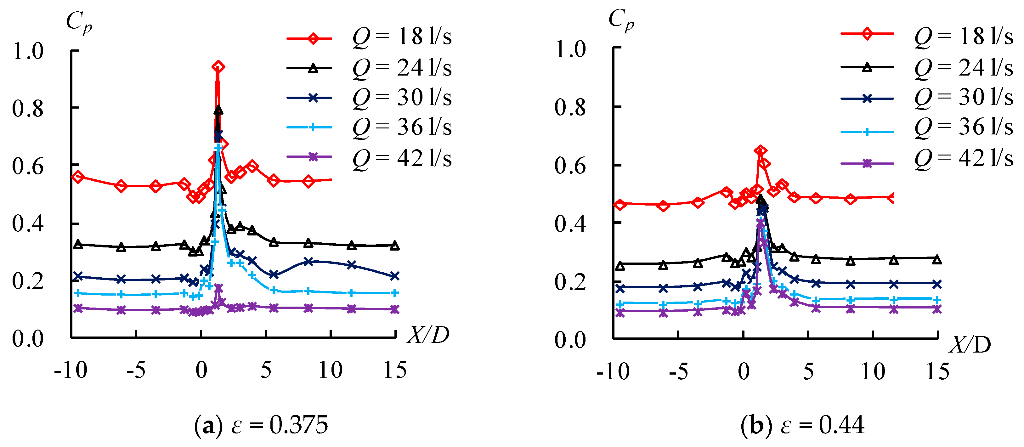
Figure 10 presents the change of Cp along the test pipe. The variation trend of Cp is similar for different ε and Q, and the peaks of Cp appear at 1.3D after the outlet of the TIED, because the TIED increases the turbulence of water flow, resulting in the enhancement of pulsating intensity near the outlet of the TIED.
Table 1 shows the greatest peak of Cp for each test group. It is clear that the peaks of Cp decrease with the increase of Q and ε, because Cp is inversely proportional to the square of Q from Equation (10) and the changing rate of pressure decreases with the increase of ε. When ε increases from 0.375 to 0.625, the averaged peak of Cp () decreases from 0.747 to 0.306 in the range of the testing flow. When Q is constant, the larger ε is, the smaller Cp is, and the larger σ is, indicating that the smaller ε is, the larger the pressure pulsation is.
3.5. Change of the Time-Averaged Velocity
The water flow in the test pipe is a turbulent flow within the test flow range, and the transient velocity of the water flow () can be divided into two parts: the time-averaged velocity () and the pulsating velocity (). The time-averaged velocity coefficient (β) is introduced to describe the characteristic of , written as:
is logarithmic distribution along the radial direction in the pipe. The value of at the center is greater than that at the side wall, and in a different position of the pipe is affected by its position and sectional geometry parameters when Q is constant.
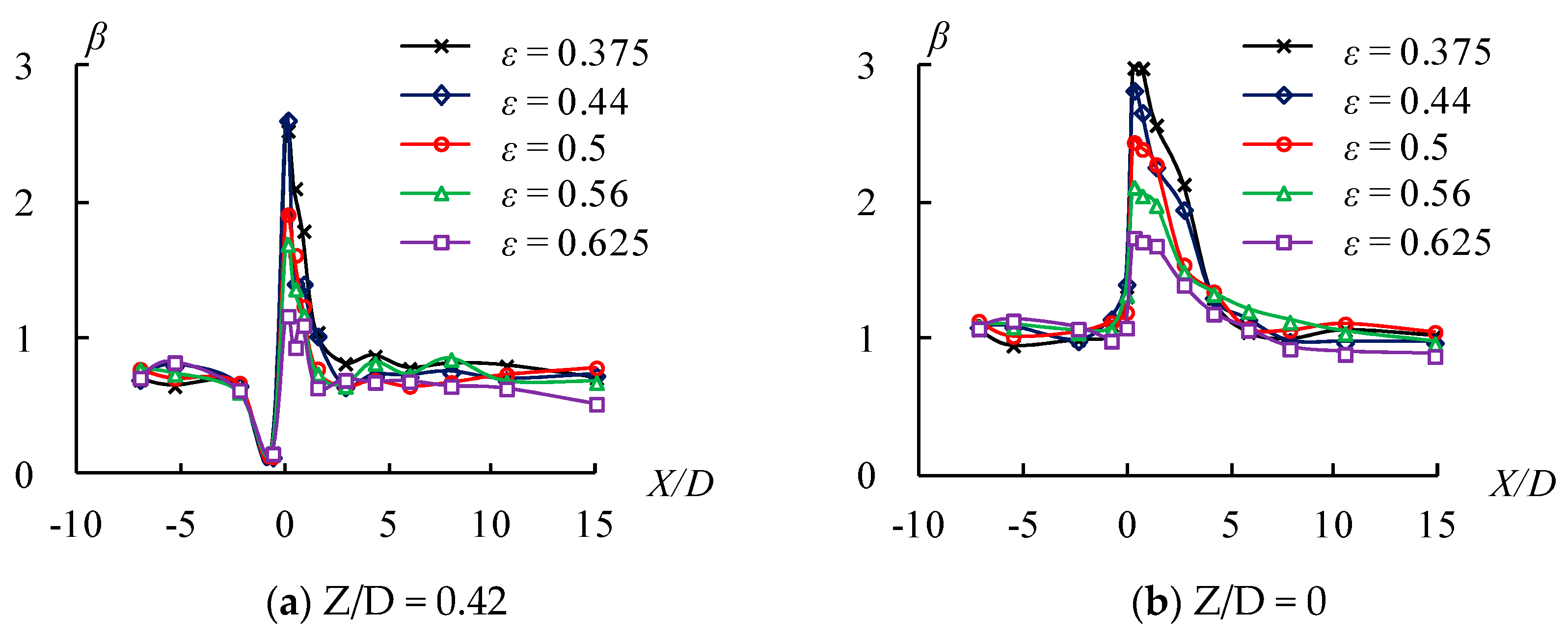
Z/D = 0 is at the central axis of the test pipe and Z/D = 0.42 is 1.2 cm away from the upper side of the test pipe. When Q is 18 l/s, the variation of β along the line of Z/D = 0 and Z/D = 0.42 for different ε is shown in Figure 11. It is clear that the change trends of β along the pipe are similar for each TIED. The values of β have little changes in the inlet and outlet sections of the test pipe, suddenly increasing at the entrance of the TIED, and then dropping sharply at the outlet of the TIED, because of the same flow cross section in the inlet and outlet sections in the test pipe and sudden changes near the TIED causing a sharp change of v. Further, the value of β on the line of Z/D = 0.42 reduced slightly before the inlet of the TIED. The value of β on the line of Z/D = 0 is larger than that on the line of Z/D = 0.42 for each measuring point. The values of β at the inlet and outlet sections of the test pipe are little affected by ε at the inlet and outlet sections of the test pipe, less than 1 on the line of Z/D = 0.42 and greater than 1 on the line of Z/D = 0. The main reason is that the inlet and outlet sections of the test pipe are far away from the TIED and is the logarithmic distribution along the radial direction in these sections. The maximum value of β is located inside the TIED. When ε increases from 0.375 to 0.625, the maximum of β near the side wall reduces from 2.53 to 1.17 on the line of Z/D = 0.42 and decreases from 2.99 to 1.74 on the line of Z/D = 0.42.
According to the comprehensive analysis, the maximum value of appears on the central axis of the pipe when X is constant. When Z is constant, the changed region of is located inside and near the TIED, and its maximum value appears inside the TIED. That is caused by the sudden decrease of the cross-sectional area for the TIED. The larger ε is, the smaller the reduced amplitude of the cross-sectional area, and the smaller β is, the smaller the maximum of .
3.6. Change of the Pulsating Velocity
The pulsating strength () is used to represent the fluctuating strength of the velocity for different measuring points and is denoted by the root mean square of the pulsating velocity ():
where N2 is the measured times of the velocity.
Introducing the turbulent strength (), and defined as:
The change of along the test pipe for different ε is illustrated in Figure 12 when Q is 18 l/s. It is shown that the variation of is similar for the different ε, and the maximum value of on the line of Z/D = 0.42 and Z/D = 0 appears at 1.57D and 2.72D away from the inlet of the TIED, respectively. ε has little effect on in the constant section of and has a great effect on the abrupt section of . When ε increases from 0.375 to 0.625, the maximum value of on the line of Z/D = 0.42 reduces from 0.68 to 0.21 and decreases from 0.56 to 0.13 on the line of Z/D = 0.
As shown in Figure 12, in the side wall is larger than that in the central axis when X is constant, which is mainly due to the diffusion of turbulent energy and the interference of the edge wall roughness causing the larger turbulence intensity at this position. The maximum value of appears after the outlet of the TIED and decreases with the increase of ε when Z is constant because of the convection of turbulent energy, resulting in downstream movement of the interference wave.
4. Conclusions
In order to gain insight into the optimized body type parameters of the TIED, the effects of the area contraction ratio (ε) on the hydraulic characteristics of the TIED were discussed using the methods of a physical model test and theoretical analysis in this paper. In the testing flow range, the main conclusions are as follows.
During the test, the flow was basically in the square area of turbulent resistance when Re changed from 1.5 × 10⁵ to 3.5 × 10⁵, and the Re had little effect on the flow characteristics. The energy dissipation rate (η) was proportional to the head loss coefficient (ξ). The flow characteristics were mainly affected by the body type of the TIED. The over-current capability () and the energy dissipation rate (η) can be characterized by and ξ, respectively. They mainly depended on ε. With the increase of ε, increased exponentially (()) and ξ decreased exponentially ( ()).
The transient pressure of turbulent flow was composed of time-averaged pressure and pulsating pressure. The change trends of time-averaged pressure coefficients (α) only depended on ε; the differences of the averaged α between the inlet and outlet of the TIED decreased from 8.2 to 1.8 when ε increased from 0.375 to 0.625 in the range of the testing flow; when the flow was about 42 l/s and ε was equal to 0.375 or 0.46, the minimum of time-averaged pressure along the pipe was negative. The pulsating pressure coefficient (Cp) was determined by Re and ε, and its peaks appeared at 1.3D after the outlet of the TIED; the averaged peaks in the range of the testing flow decreased from 0.747 to 0.306 when ε increased from 0.375 to 0.625. Negative pressure and larger peaks of pulsating pressure coefficient were more prone to cavitations behind the outlet of TIED.
The transient velocity of turbulent flow was divided into time-averaged velocity and pulsating velocity, which can be represented by time-averaged flow velocity coefficients (β) and turbulent strength (Tu), respectively. When X was constant, the maximum of β appeared on the line of Z/D =0 in pipe, and β near the side wall was larger than that on the line of Z/D =0 in pipe due to the diffusion of turbulent energy and the interference of the wall roughness. When Z was constant, the maximum value of β appeared inside the TIED for different ε, decreasing with the increase of ε. Moreover, the maximum value of Tu appeared after the outlet of the TIED and decreased with the increase of ε because of the convection of turbulent energy. Therefore, the smaller ε is, the more likely it is that cavitations occur near the pipe wall behind the outlet of the TIED.
Comprehensive analysis of over-current capability, energy dissipation rate, and the distribution of flow velocity and pressure showed that the optimized body type parameter (ε) of the TIED in the test was 0.5 when flow in the pipe was about 42 l/s.
Author Contributions
T.Z., designed and performed the model test, and wrote the preliminary manuscript paper; Z.Z., conducted preparation of experiment and preliminary analysis the data of model test; R.H. and X.Z., provided guidance for model test and also further improved the concept, structure, contents and writing of the preliminary manuscript paper.
Funding
This work was supported by the Natural Science Foundation of Shanxi Province (Grand No: 2013011037-4) and National Natural Science Foundation of China (Grant No.51109155).
Conflicts of Interest
The authors declare no conflict of interest.
References
- Fossa, M.; Guglielmini, G. Pressure drop and void fraction profiles during horizontal flow through thin and thick orifices. Exp. Therm. Fluid Sci. 2002, 26, 513–523. [Google Scholar] [CrossRef]
- Wu, J.H.; Ai, W.Z. Flows through energy dissipaters with sudden reduction and sudden enlargement forms. J. Hydrodyn. 2010, 22, 360–365. [Google Scholar] [CrossRef]
- Ai, W.Z.; Hu, L. Research on energy dissipation in a discharge tunnel with a plug energy dissipater. Trans. Famena 2016, 40, 57–66. [Google Scholar]
- Tian, Z.; Xu, W.L.; Wang, W.; Liu, S.J. Hydraulic characteristics of plug energy dissipater in flood discharge tunnel. J. Hydrodyn. 2009, 21, 799–806. [Google Scholar] [CrossRef]
- Wu, J.; Ai, W.Z.; Zhou, Q. Head loss coefficient of orifice plate energy dissipator. J. Hydraul. Res. 2010, 48, 526–530. [Google Scholar]
- Yu, T.; Tian, Z.; Wang, W.; Xu, W.L. Energy dissipation and cavitation characteristics of contracted plug in discharge tunnel. J. Hydraul. Eng. 2011, 42, 211–217. [Google Scholar]
- Lian, L.; Wang, W.; Tian, Z. Characteristics of energy dissipation and cavitation for complex plug in discharge tunnel. J. Hydroelectr. Eng. 2012, 2, 62–70. [Google Scholar]
- Rydlewicz, W.; Rydlewicz, M.; Pałczyński, T. Experimental investigation of the influence of an orifice plate on the pressure pulsation amplitude in the pulsating flow in a straight pipe. Mech. Syst. Signal Process. 2019, 117, 634–652. [Google Scholar] [CrossRef]
- Roul, M.K.; Dash, S.K. Single-phase and two-phase flow through thin and thick orifices in horizontal pipes. J. Fluids Eng. Trans. ASME 2012, 134, 091301. [Google Scholar] [CrossRef]
- Ai, W.Z.; Wang, J.H. Minimum wall pressure coefficient of orifice plate energy dissipater. Water Sci. Eng. 2015, 8, 85–88. [Google Scholar] [CrossRef] [Green Version]
- Dong, J.; Xu, W.; Deng, J.; Liu, S.; Wang, W.; Qu, J. Numerical simulation of turbulent flow through throat-type energy-dissipators. J. Hydrodyn. Ser. B 2002, 14, 135–138. [Google Scholar]
- Tian, Z.; Deng, J.; Feng, X. Investigation of flow field of plug dissipaters by LDV. J. Sichuan Univ. (Eng. Sci. Ed.) 2014, 46, 1–5. [Google Scholar]
- Ai, W.Z.; Ding, T.M. Orifice plate cavitation mechanism and its influencing factors. Water Sci. Eng. 2010, 3, 321–330. [Google Scholar]
- Zhou, H. Numerical analysis of the 3-D flow field of pressure atomizers with V-shaped cut at orifice. J. Hydrodyn. Ser. B 2011, 23, 187–192. [Google Scholar] [CrossRef]
- Zhang, C.-B.; Yang, Y.-Q. 3-D numerical simulation of flow through an orifice spillway tunnel. J. Hydrodyn. Ser. B 2002, 14, 83–90. [Google Scholar]
- Zhang, T.; Tian, C.; Li, Y.; You, Z.; Fan, P. Characteristics of energy dissipation and pressure within inner energy dissipaters of tooth block. J. Drain. Irrig. Mach. Eng. 2014, 32, 136–139. (In Chinese) [Google Scholar]
- Xue, D.; Tian, C. Influence of energy dissipation efficiency for different area reduction ratio on tooth pier energy dissipation. Water Resour. Power 2014, 4, 84–87. (In Chinese) [Google Scholar]
- Jiang, X.; Hao, R.; Li, Y. Study on pressure and flow field characteristics of tooth block inner energy dissipater. Water Resour. Power 2015, 8, 94–97. (In Chinese) [Google Scholar]
- Su, D.; Hao, R. Numerical simulation of hydraulic characteristic of tooth-block inner energy dissipaters. Water Resour. Power 2015, 11, 79–81. (In Chinese) [Google Scholar]
- Yin, Z.; Shi, B.; Zhao, L.; Sun, D. Numerical simulation of plug energy dissipater flow. Adv. Water Sci. 2008, 1, 89–93. [Google Scholar]
- Li, X. Numerical Simulation on Influence of Flow Characteristics for the Dental Length on Tooth Block Inner Dissipater. Master’s Thesis, Taiyuan University of Technology, Taiyuan, China, October 2015. [Google Scholar]
- Wang, H. Experimental Research about Tooth Block Height Effect on Inner Energy Dissipaters of Tooth Block. Master’s Thesis, Taiyuan University of Technology, Taiyuan, China, October 2015. [Google Scholar]
Figure 1.
Layout of test pipe.

Figure 2.
Cross-sectional areas of toothed internal energy dissipaters (TIED).

Figure 3.
The distribution of measuring points along the test pipe.

Figure 4.
Relationship of the flow coefficient () and area contraction ratio (ε).

Figure 5.
Relationship between the measured or calculated values of the averaged flow coefficient () and the area contraction ratio (ε).
Figure 5.
Relationship between the measured or calculated values of the averaged flow coefficient () and the area contraction ratio (ε).

Figure 6.
Relationship of the energy dissipation rate (η) and area contraction ratio (ε).

Figure 7.
Relationship between the measured or calculated averaged value of the head loss coefficient () and the area contraction ratio (ε).
Figure 7.
Relationship between the measured or calculated averaged value of the head loss coefficient () and the area contraction ratio (ε).

Figure 8.
Distribution of time-averaged pressure coefficient (α) and the mean of time-averaged pressure coefficient () along the test pipe.
Figure 8.
Distribution of time-averaged pressure coefficient (α) and the mean of time-averaged pressure coefficient () along the test pipe.

Figure 9.
Relationship between the mean of time-averaged pressure coefficient () and the area contraction ratio (ε).
Figure 9.
Relationship between the mean of time-averaged pressure coefficient () and the area contraction ratio (ε).

Figure 10.
Distribution of pulsating pressure coefficient along for the typical body type of the TIED.
Figure 10.
Distribution of pulsating pressure coefficient along for the typical body type of the TIED.

Figure 11.
Changes of the time-averaged velocity along the test pipe.

Figure 12.
Distribution of turbulent strength along the test pipe.


Table 1.
Peaks and average values of pulsating pressure coefficient for each test group.
| ε Cpmax Q | 0.375 | 0.44 | 0.5 | 0.56 | 0.625 |
|---|---|---|---|---|---|
| 18 | 0.942 | 0.654 | 0.652 | 0.644 | 0.64 |
| 24 | 0.794 | 0.489 | 0.355 | 0.355 | 0.316 |
| 30 | 0.707 | 0.442 | 0.282 | 0.272 | 0.233 |
| 36 | 0.661 | 0.413 | 0.268 | 0.216 | 0.184 |
| 42 | 0.633 | 0.405 | 0.247 | 0.203 | 0.16 |
| 0.747 | 0.48 | 0.361 | 0.338 | 0.306 |
© 2019 by the authors. Licensee MDPI, Basel, Switzerland. This article is an open access article distributed under the terms and conditions of the Creative Commons Attribution (CC BY) license (http://creativecommons.org/licenses/by/4.0/).
Share and Cite
MDPI and ACS Style
Zhang, T.; Hao, R.-x.; Zheng, X.-q.; Zhang, Z. Effect of the Area Contraction Ratio on the Hydraulic Characteristics of the Toothed Internal Energy Dissipaters. Water 2019, 11, 1406. https://doi.org/10.3390/w11071406
AMA Style
Zhang T, Hao R-x, Zheng X-q, Zhang Z. Effect of the Area Contraction Ratio on the Hydraulic Characteristics of the Toothed Internal Energy Dissipaters. Water. 2019; 11(7):1406. https://doi.org/10.3390/w11071406
Chicago/Turabian StyleZhang, Ting, Rui-xia Hao, Xiu-qing Zheng, and Ze Zhang. 2019. "Effect of the Area Contraction Ratio on the Hydraulic Characteristics of the Toothed Internal Energy Dissipaters" Water 11, no. 7: 1406. https://doi.org/10.3390/w11071406
Note that from the first issue of 2016, this journal uses article numbers instead of page numbers. See further details here.