Article

Identification of Sulfate Sources and Biogeochemical Processes in an Aquifer Affected by Peatland: Insights from Monitoring the Isotopic Composition of Groundwater Sulfate in Kampinos National Park, Poland

1
Institute of Geological Sciences Polish Academy of Sciences (ING PAN), Ul. Twarda 51/55, 00-818 Warszawa, Poland
2
Faculty of Geology, University of Warsaw, Ul. Żwirki i Wigury 93, 02-089 Warsaw, Poland
3
Mass Spectrometry Laboratory, Maria Curie-Skłodowska University, plac M. Curie-Skłodowskiej 1, 20-031 Lublin, Poland
*
Author to whom correspondence should be addressed.
Stanislaw Halas passed away in 2017.
Water 2019, 11(7), 1388; https://doi.org/10.3390/w11071388
Submission received: 28 May 2019 / Revised: 22 June 2019 / Accepted: 29 June 2019 / Published: 5 July 2019
(This article belongs to the Special Issue Use of Water Stable Isotopes in Hydrological Process)

Abstract

:
Temporal and spatial variations of the concentration and the isotopic composition of groundwater sulfate in an unconfined sandy aquifer covered by peatland have been studied to better understand the sources and biogeochemical processes that affect sulfate distribution in shallow groundwater systems influenced by organic rich sediments. The groundwater monitoring was carried out for one year at hydrogeological station Pożary located within the protected zone of the Kampinos National Park. Sulfur (δ34SSO4) and oxygen (δ18OSO4) isotopic composition of dissolved sulfates were analyzed together with oxygen (δ18OH2O) and hydrogen (δ2HH2O) isotopic composition of water and major ions concentration at monthly intervals. The research revealed three main sources of sulfates dissolved in groundwater, namely, (a) atmospheric sulfates—supplied to the aquifer by atmospheric deposition (rain and snow melt), (b) sulfates formed by dissolution of evaporite sulfate minerals, mainly gypsum—considerably enriched in 34S and 18O, and (c) sulfate formed during oxidation of reduced inorganic sulfur compounds (RIS), mainly pyrite—depleted in 34S and 18O. The final isotopic composition and concentration of dissolved SO42− in groundwater are the result of overlapping processes of dissimilatory sulfate reduction, oxidation of sulfide minerals, and mixing of water in aquifer profile.

Graphical Abstract

1. Introduction

Organic-rich sediments in hydrogeological profile, their high productivity and complex biogeochemistry have a globally significant influence on the quality of adjacent groundwaters, their chemical composition, trace elements cycling and the composition of atmospheric trace gases [1]. Wetlands, bogs, fens, and peatlands, which cover nearly 5% of the Earth’s surface, are such ecosystems where the accumulation of reactive organic matter always implies a series of redox processes which control not only the content of carbon in groundwater but also the distribution of major dissolved compounds, including, for example, nitrogen or sulfur species [1,2,3,4,5,6,7,8,9,10,11,12,13]. Peatlands are very heterogeneous environments: inside the peatland bed, macro and micro gradients of redox conditions enable the development of a highly diverse microbial community capable of different redox reactions occurring simultaneously (e.g., nitrification, denitrification, sulfate reduction, oxidation of reduced inorganic sulfides, etc.) on a small spatial scale [7,9,10]. The biotic and abiotic transformations of sulfur compounds are interconnected with other geochemical processes through their common substrates or products. Sulfates reduction in peatlands can result in Eh and pH changes in groundwater, alkalinity generation, and C transformation, and, indirectly, the mobilization and removal of nutrients such as N, P, and C [2,3,6,7]. Moreover, sulfide as a product of dissimilatory sulfate reduction may remove heavy metals contained in waters via the formation of metal sulfides.
Numerous studies concerning wetland systems are focused first of all on the investigation of sulfur compounds transformation, sulfate reduction and generation directly in the organic-reach beds under environmentally relevant conditions in order to better understand the overall sulfur cycle dynamic and net sulfur compounds storage within freshwater peatlands [1,7,9,10,13,14]. Some of these researches are aimed at the direct application of wetlands to natural restoration of water quality e.g., [1,9]. An important part of the sulfur cycle in peatland systems involves the formation and sink of the organic sulfur species, the formation of biogenic minerals, and the interaction between mineral matter and organic matter [4,6,10].
Stable isotopes of O and S are used first of all to investigate the sulfate sources, the sulfate reduction and oxidation zones in the peat, and to compare sulfate sources in various wetland systems often located in different hydrogeological and climatic conditions [4,5,7,14]. Isotopic composition of sulfates is also used to explain the mechanisms and sources of SO42− released from peatlands to streams, lakes, or soils [11,13,14].
Still insufficient attention is addressed to investigation the long term, direct influence of the peatland ecosystems on the geochemistry of groundwater masses in adjacent aquifers, especially in changing climate conditions. In this study we utilize an approach involving O and S isotopic composition of sulfates to identify the sulfate sources and biogeochemical processes that affect sulfate distribution in a shallow alluvial aquifer covered by peatland. The research was performed at the Pożary monitoring station, located in an area of Holocene peats of the Vistula River terrace in the Kampinos National Park, Central Poland (52°17’5” N, 20°29’4” E). The monitoring station was equipped with four piezometers installed at different depths in a sandy aquifer, namely 2.1, 3.3, 4.75, and 8.35 m (Figure 1). A previous study performed in this area by Porowska and Lesniak [15] focused on the distribution of dissolved inorganic carbon (DIC) and its C isotope composition, as well as on dissolved organic carbon (DOC) and dissolved oxygen (DO) in the aquifer profile. The study indicated that the mineralization of organic matter and the presence of organic carbon in the geological profile may have a significant effect on the biogeochemical processes controlling the chemical composition of groundwater in the aquifer. For example, the concentration of dissolved sulfate showed one of the largest seasonal variations in comparison to other major constituents. Seasonal and spatial variation of sulfates concentration and their stable O and S isotopic compositions is an important tracer of the sulfate sources, the biogeochemical processes in groundwater environment, and the geochemical conditions in the aquifer [4,11,12].
The major forms of sulfur in the hydrogeological subsurface environment include sulfate (SO42−) and sulfide (HS) minerals, sulfate and sulfide dissolved in water, and hydrogen sulfide gas (H2S) and sulfur in organic compounds (DOS) [2,3]. These various sources of sulfur may participate in the evolution of the chemical composition of water masses below the ground. Dissolved sulfates (SO42−) are usually the dominant form of sulfur, and are one of the most common sulfur species in various natural groundwater environments. The geochemistry of sulfur is complicated by its wide range of oxidation states. However, the key reaction in the global sulfur cycle, i.e., the reduction of sulfate (SO42− to hydrogen sulfide (H2S), may be identified by the distribution of sulfate concentrations and its O and S isotopic composition. When sulfate ions reach the anaerobic zone within the saturated soil, peatland or groundwater, the sulfate reducing bacteria start producing sulfides (S2−); consequently, the concentration of dissolved SO42− in water decreases and considerable fractionation of 34S/32S and 18O/16O isotope occurs. The residual SO42− becomes progressively enriched in the heavy isotopes 18O and 34S [5,7,9,11].
This paper gives the results of a thorough one-year monitoring study of the concentration of dissolved sulfate and its sulfur (δ34S) and oxygen (δ18O) isotopic composition together with the chemical and isotopic (δ2H and δ18O) composition of groundwater in the aquifer vertical profile. The performed study had three principal objectives, namely (i) to distinguish between sulfate sources in the groundwater of the shallow unconfined aquifer covered by peatland, (ii) to identify the biogeochemical processes controlling the distribution and isotopic transformation of sulfates in the shallow groundwater system, and (iii) to evaluate the influence of organic-rich sediments on the geochemical conditions in the groundwater flow system. Explaining these phenomena is essential to obtain a better understanding of the sulfur cycling between the peat and the groundwater, and the influence of organic-rich sediments on the evolution of water chemistry in adjacent unconfined aquifers.

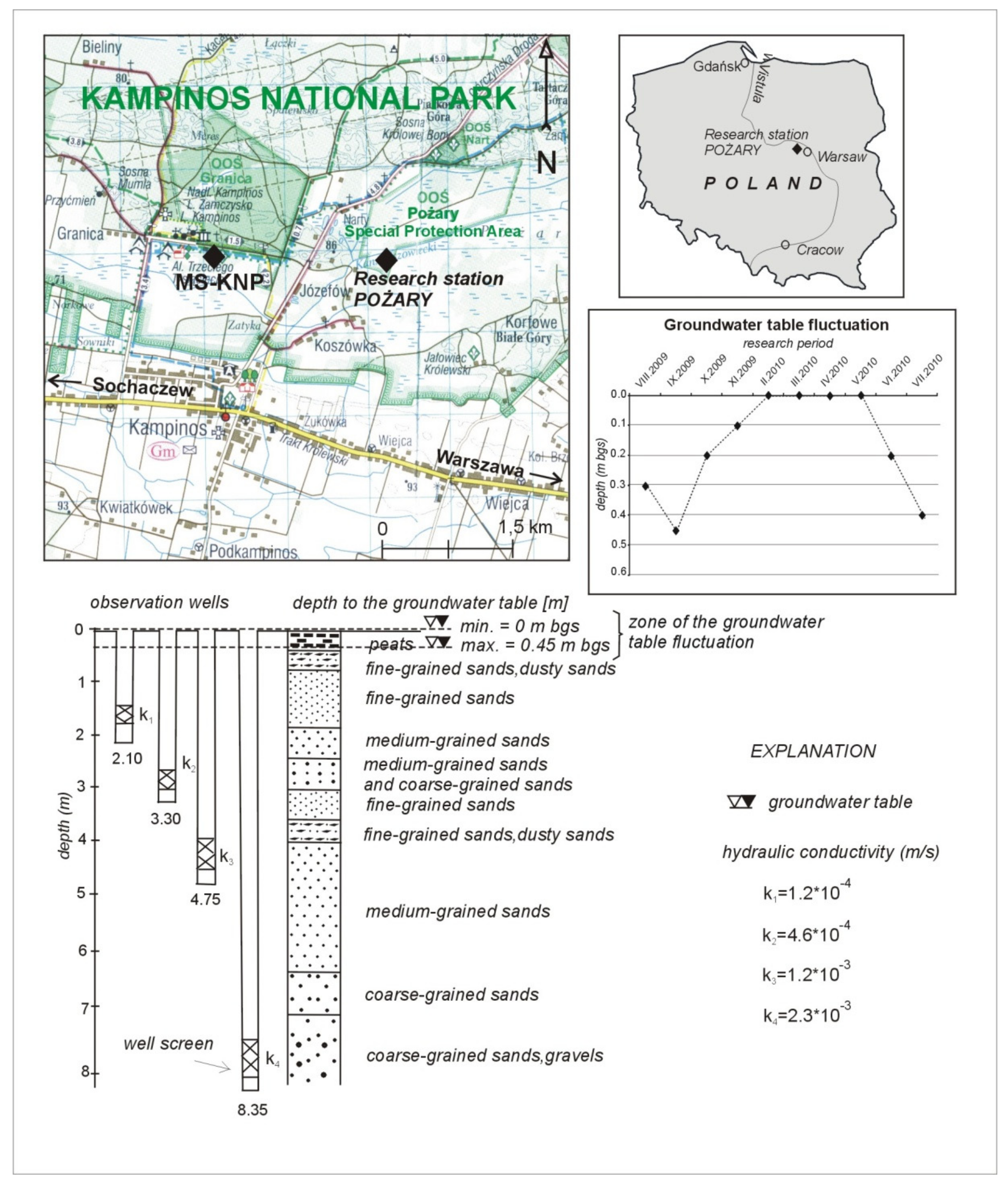
2. Study Area and Hydrogeological Settings

Kampinos National Park, located several kilometers northwest of Warsaw, Poland, is a special protection area where extensive ecological and climatic studies have been conducted for several years. There is one fully equipped meteorological station in this area, as well as several smaller research stations where only piezometers or observation wells are installed to monitor the level and the quality of groundwater for the needs of the Polish National Groundwater Monitoring Network. Our investigation was performed at the Pożary research station, located in an area of Holocene peats on the Vistula River terrace (Figure 1) [16]. The research station was equipped with four piezometers installed in the same aquifer at different depths. The shallowest one (depth: 2.10 m) was installed at a contact between fine- and medium-grained sands. The next two piezometers (depths: 3.30 and 4.75 m) were set into medium-grained sands, and the deepest one (depth: 8.35 m) was set into coarse-grained sands and gravels (Figure 1). The organic matter was accumulated within a peat layer with a thickness of 0.5 m in the uppermost part of the geological profile, within the vadose zone.
Depending on the season and position of the groundwater level, the layer of peat may occur within either the saturation or vadose zone. During the one year of monitoring studies, the groundwater table fluctuated in the range from 0.0 to 0.45 m below ground surface (bgs). Generally, the groundwater level was above the peat surface during winter and spring, i.e., from February 2009 to May 2010, and was below the ground surface at depths from 0.10 to 0.45 m during summer and autumn, i.e., from August 2009 to November 2009 and from June 2010 to July 2010. It is important to note that the capillary fringe in the peat can extend to 0.2 m above the water table [18]. The hydraulic conductivity in the aquifer increases with depth, from 1.2·10−4 to 2.3·10−3 m/s (Figure 1)

3. Materials and Methods

Samples of groundwater were collected from four observation piezometers installed close to each other in the same aquifer. The piezometers were simple PVC standpipes slotted in the saturated zone at various depths, i.e., 2.1 (the shallowest one), 3.30, 4.75, and 8.35 m (the deepest one). The samples of groundwater were collected at monthly intervals from August 2009 to July 2010. In December 2009 and January 2010, the field campaign was suspended due to harsh weather and thick snow cover, which caused the piezometers and groundwater to be unavailable for sampling. To collect representative samples of water from the aquifer, sampling procedures were strictly followed [19,20,21,22]. Field measurements were made of basic physicochemical water quality parameters such as temperature (T), pH, electrical conductivity (EC), and oxygen/reduction potential (ORP), using a small electrical water pump, an in-line flow-through cell, and portable meters such as a HQ40D multi meter (Hach®, Hach-Lange GMBH, Berlin, Germany) equipped with Intellical (Hach-Lange GMBH, Berlin, Germany) pH, EC, and ORP electrodes with temperature sensors. The EC and ORP values were used to determine when formation-quality water was available for sample collection [20].
For chemical analysis, water was filtered through 0.7 μm GF/F (glass microfiber) Whatman’s syringe filters and collected in polyethylene bottles—150 mL aliquots for anions and 30 mL aliquots for cations. Then, bottles were put into a refrigerator and delivered to the laboratory within 48 h. A High-Performance Liquid Chromatography (HPLC) method was used for major anion analysis (except bicarbonates and nitrates), and the Inductively Coupled Plasma Absorption Emission Spectrometry (ICP-AES) method was used for cation analysis. Uncertainties in the determination of major ions, as reported by the laboratory, were in the range 5–10%. Bicarbonates were determined by the potentiometric titration method, and concentrations of NO3 were determined in the field using a Slandi LF portable spectrophotometer (SLANDI®, SLANDI sp. z o.o., Michalowice, Poland). The anion-cation charge balance method was followed to assess the accuracy of the chemical analyses: for all water samples, the charge balance was less than 5%. The chemical analyses were performed at the Institute of Environmental Protection, National Research Institute in Warsaw, Poland. Table 1 shows a compilation of the physicochemical data obtained for groundwater.
Water samples for the analysis of oxygen stable isotope and hydrogen composition were collected in 30 mL amber-glass bottles and tightly sealed. Routine mass spectrometric techniques were applied for the determination of the isotopic composition of water, namely an off-line technique of CO2–H2O equilibration [23,24] to determine 18O/16O ratios, and an off-line static batch water reduction on hot zinc to determine 2H/1H ratios [25,26,27,28]. The results were reported using δ notation with respect to the VSMOW international standard. Normalization of measured data was perform according to three international standards, namely: VSMOW (δ2H = 0.0‰, δ18O = 0.0‰), VSLAP (δ2H = −427.5‰, δ18O = −55.50‰), and GISP (δ2H = −189.5‰, δ18O = −24.76‰). The precision of the measurements was ±0.08‰ and ±0.9‰ for δ18O and δ2H, respectively. The precision of the isotopic measurements was calculated based on long-term measurements of international reference materials as well as our internal standard water. The analyses were performed at the Institute of Geological Sciences of the Polish Academy of Sciences (ING PAN) in Warsaw, Poland.
Water samples for the analysis of the stable isotopes of sulfur (34S/32S ratio) and oxygen (18O/16O ratio) of dissolved sulfates were collected in HDPE bottles with volumes of 1 or 2 L depending on SO42− concentration, which was determined in the field using a Slandi LF portable spectrophotometer. Afterwards, the water samples were acidified to a pH of 2–3 and an appropriate amount of 10% BaCl solution was added in order to precipitate all dissolved sulfates as BaSO4 [29]. A method based on the reduction of BaSO4 with graphite to CO2 was applied to determine the 18O/16O ratio of sulfates [30,31], while a method for the conversion of BaSO4 to SO2 at 850 °C was applied to determine the 34S/32S ratio [32]. The results of the analysis were reported using δ notation: δ18O with respect to VSMOW and δ34S with respect to VCDT. Normalization of measured data was perform according to international standards, namely: NBS-127 (δ34S = +20.3‰ VCDT, δ18O = +9.3‰ VSMOW) and IAEA-SO6 (δ34S = −34.1‰ VCDT, δ18O = −11.35‰ VSMOW). The precision of the measurements was ±0.1 ‰ for both δ18O and δ34S. The analyses of the isotopic composition of sulfates were performed in the Laboratory of Mass Spectrometry at the Institute of Physics UMCS, Lublin, Poland. Table 2 shows a compilation of the isotopic data obtained for groundwater.
The PHREEQC software provided by the USGS (version 2.13.2 with the minteq.dat thermodynamic database), was used to calculate saturation indices (SIs) for selected minerals.
Together with groundwater, rainwater samples were collected and analyzed in order to determine the chemical and isotopic composition of atmospheric precipitation, which is the major input (recharge) component in the studied groundwater system. Rainwater samples were obtained from the meteorological station of Integrated Monitoring of the Natural Environment of Kampinos National Park (52°17′10″ N, 20°27′17″ E), located about 2 km west of the Pożary research station. A standard Hellmann’s rain gauge was used to collect and measure atmospheric precipitation. Monthly cumulative rainwater was collected in separate polyethylene bottles with volumes of 1–2 L (one for each month), which were stored in a refrigerator at a temperature of 4 °C and subjected to the same set of chemical and isotopic analyses together with groundwater obtained from the piezometers. Physicochemical parameters of the rainwater were measured in the field during each water collection.
Table 1 and Table 2 show data obtained for the rainwater samples. In order to present the entire vertical profile of the chemical and isotopic composition of atmospheric precipitation and groundwater, the data for rainwater are presented for a depth of 0.0 m in plots of Section 4.

4. Results

Chemical analyses of groundwater and rainwater were made six times during an entire monitoring period. The results are presented in Table 1.
Variations of groundwater temperature, pH, ORP, and EC at different depths are presented in Figure 2. The groundwater temperature in the Pożary aquifer varied between 8.9 and 17.2 °C, depending on the seasonal ambient air temperature (Figure 2). The pH of the groundwater ranged from 6.56 to 7.16, indicating slightly acidic and neutral conditions. Taking into account the vertical profile, the lowest pH values in the range of 4.44–5.87 are characteristic of atmospheric precipitation (i.e., rain and snow). In groundwater, the pH is higher than that of precipitation, and clearly varies with depth: It was highest in the upper part of the aquifer (pH > 7.0) and then decreased, reaching the lowest values in the middle part, before again reaching higher values in the deeper part (Figure 2). The EC of groundwater ranged from 484 to 780 µS/cm, and varied with depth, repeating the trend characteristic for pH.
The ORP varied between −28 and +109 mV, depending on the season and sampling depth. The lowest values occurred at 2.10 m bgs, indicating slightly reducing conditions (from −28 to 60 mV), probably due to the influence of the microbial decomposition of organic matter in the peat layer. In the deeper parts of the aquifer, positive values of redox potential were observed (from 14 to 109 mV), indicating a mildly reducing environment.
The hydrogeochemical type of the water in the aquifer changes with depth as a result of the variation in the concentration of major anions (Figure 3 and Figure 4). In the upper part of the aquifer, water of HCO3-Ca type dominates. In the middle part, at a depth of 3.3 m, the concentrations of the major anions change abruptly: The content of HCO3 reaches the minimum, the contents of SO42− and Cl reach the maximum, and the hydrogeochemical type of the water evolves into HCO3-Cl-SO4-Ca or HCO3-SO4-Cl-Ca. In the deeper parts of the aquifer, the concentration of HCO3 gradually increases, whereas the contents of SO42− and Cl decrease abruptly at a depth of 4.75 m before beginning to rise again with depth; from a depth of 4.75 m, water of the HCO3-SO4-Ca type dominates (Figure 3 and Figure 4). On the other hand, at a depth of 3.3 m, the concentrations of major cations (Ca2+, Mg2+, and Na+) usually exhibit the lowest values, which remain stable or rise slightly in deeper parts of the aquifer. A comparison of archival and actual data of the chemical composition of groundwater shows similar trends of evolution with depth (Figure 3).
The variation in the stable isotope compositions of groundwater (δ18O and δ2H) and dissolved sulfates (δ34S and δ18O) with depth in the aquifer are summarized in Table 2 and Figure 4.
Typically, the oxygen and hydrogen isotopic composition of groundwater generally reflects the mean weighted annual composition of precipitation. In our case of a shallow unconfined aquifer with a relatively thin unsaturated zone (i.e., about 0.5 m in thickness) composed of a peat layer, the large seasonal variations of the O and H isotopic composition of precipitation are considerably attenuated in the upper part of the saturated zone. For example, the variation coefficient of δ18O in the precipitation (rain and snow) reached about 35%; while at a depth of 2.1 m, seasonal variations were attenuated to about 2% (Figure 4). The isotopic composition of dissolved sulfates in atmospheric precipitation was measured three times: Two times in rain water, with each value representing rain water collected over a few months (due to a relatively low concentration of dissolved sulfates and the small amount of water available after each month), and one time in snow in December.
The obtained values of isotopic composition (Table 2) are typical for the fallout in rural areas (e.g., [12]). The isotopic composition of SO42− dissolved in groundwater ranged from −2.6 to +20.9‰ and from +5.1 to +16.8‰ for δ34SSO4 and δ18OSO4, respectively. As can be seen from Figure 4, both δ34SSO4 and δ18OSO4 demonstrate significant variation along the depth profile. Generally, the observed vertical variation trend of the isotopic composition of SO42− is reversed compared to that of SO42− concentration. Sulfates were most depleted in 34S and 18O at a depth of 3.30 m in almost all of the observation period (Figure 4). At a depth of 3.30 m, the values of δ34SSO4 gradually decreased from September 2009 to April 2010, before increasing from April 2010 to July 2010. For δ18OSO4, a seasonal trend similar to that of δ34SSO4 was observed.

5. Discussion

The chemical composition of subsurface water is always a complex function of many variables, e.g., the composition of recharge, the mineralogy and composition of the geological environment, and the hydrogeological and hydraulic settings. One of the main factors affecting groundwater chemistry is the presence of organic matter. The mineralization (oxidation) of organic matter in soil and aquifer environments always implies a series of redox reactions which control the distribution of major species dissolved in groundwater, with the organic matter being the major reductant [2,3,4,5,6,7].
As long as free oxygen is available in the saturated zone, the simplified reaction of organic matter oxidation can be written as follows:
CH2O + O2 → CO2 + H2O
During this process, firstly carbon is released as CO2. Depending on the reactivity and composition of organic matter, a combination of organic NO3 and HPO42− can also be released to groundwater. The concentrations of NO3 and HPO42− have not been studied in detail in the aquifer of the Pożary research station. However, clear evidence of organic matter decomposition in the aquifer vertical profile was shown by Porowska and Leśniak [15]—namely, an increase in CO2 partial pressure and DIC content with a carbon isotopic composition typical of organic origin (reported δ13C from −17 to −25‰ vs. PDB), an increase in organic carbon concentration (DOC), and a decrease in oxygen content (DO, reported concentrations range from 0.48–1.62 mg/dm3). An additional consequence of the increase in CO2 concentration in the upper part of the aquifer is an increase in the weathering capacity of groundwater and the induction of carbonate mineral dissolution, which may result, for example, in an increase in Ca and Mg concentrations (see Figure 4).
Water saturation promotes anoxic conditions in soil, vadose zone, or an aquifer. When molecular oxygen is not available (i.e., when it has been used up), the oxidation of organic matter continues and terminal electron acceptors other than O2 are utilized. Depending on redox potential, pH, and availability of electron acceptors, the following microbial reduction processes can occur after O2 depletion (i.e. the sequential reduction chain—a series of reactions which represent successively lower Eh levels): Nitrate, manganese, iron, sulfate, and finally CO2 [7]. The reduction of NO3 by organic matter (denitrification) is a bacterially catalyzed process, it starts the sequential reduction chain in the aquifer, and can be written as an overall reaction (after [3]):
5CH2O +4NO3 → 2N2 +4HCO3 + CO2 +3H2O
Denitrification predominantly proceeds to the final product of N2 [8,34,35,36,37]. An additional consequence of this process is the increase of HCO3 concentration and pH values (e.g., see the upper part of the profile up to 2.1 m in Figure 2 and Figure 4). Different forms of nitrogen in shallow groundwater in wetlands and peat bogs of the Kampinos National Park were studied by Krogulec and Jóźwiak [38]. They typically reported very low concentrations of NO3 (from 0 mg/dm3 to a maximum of 5.3 mg/dm3) as a result of denitrification. Our research corroborates their conclusions: The concentration of NO3 in the groundwater of the Pożary aquifer was below 0.5 mg/dm3 (see Table 1). Taking into account the aquifer profile below the peat layer, the transition between the denitrification zone and the sulfate reduction zone most likely occurs in the depth range from 2–4 m bgs: Here, the sulfate concentration starts to decrease and the HCO3 concentration starts to rise with depth (Figure 3).
The geochemical modeling of sulfur speciation (based on PHREEQC software) shows that sulfate is the main species of sulfur in the groundwater studied. The groundwater sulfates may be derived from various sources, such as atmospheric, pedospheric, lithospheric, and anthropogenic. In shallow aquifers in peatland areas, the sources of sulfate are usually pyrite, gypsum, biogenic sulfur compounds contained in the peat (mostly lithospheric sources), and atmospheric deposition [3,5,6,9,39,40].
However, the concentration, as well as the sulfur and oxygen isotopic composition, of sulfates in groundwater are controlled not only by sulfate sources but also by subsequent biotic and abiotic processes in the aquifer, including hydraulic conditions (e.g., groundwater mixing, fluctuation of ground water level, lateral flow). Hence, four processes may potentially control the distribution and isotope signatures of dissolved sulfate in the Pożary aquifer: (1) Bacterial (dissimilatory) sulfate reduction; (2) the formation and oxidation of reduced inorganic sulfur (RIS); (3) the dissolution of evaporitic sulfates (mainly gypsum); and (4) the mixing of sulfate from different sources. All of these processes result in specific patterns of the concentration and isotopic composition of dissolved SO42−, and in favorable hydrogeological settings can be identified by geochemical and isotopic techniques.

5.1. Sulfate Sources in Groundwater Studied

The sources of sulfate in groundwater can have a wide range of δ34S values. Usually, the local source of sulfate in groundwater is estimated using the relationship between δ34S and the concentration of dissolved sulfate [12,41,42,43]. Plotting the δ34S values of groundwater sulfate versus the inverse of sulfate concentration (1/[SO42−]) for all water samples yielded a straight line with a correlation factor (R2) of 0.6 and a y-axis intercept of −7.9‰ (Figure 5A).
The slope of the line s equals
s = CR × (δ34SR − δ34SI)
where CR refers to the concentration of the remaining (i.e., measured) sulfate, and δR and δI refer to the sulfur isotopic composition of the remaining (i.e., measured) and initial (i.e., source) sulfate, respectively. The y-axis intercept represents δI.
The y-axis intercept indicates the sulfur isotopic composition of the potential source of groundwater sulfates. The value of −7.9‰ strongly suggests that the RIS compounds are the dominant lithogenic source responsible for increasing the sulfate concentration in the groundwater of the Pożary aquifer. However, a more detailed picture of the sulfate sources can be obtained by taking into account the entire observation period and the variation of sulfate concentration and sulfur isotopic composition separately in the monitored respective depths of the aquifer (Figure 5B).
The most extreme relationships were observed for groundwater sulfates at depths of 2.1 and 3.3 m. The y-axis intercept for sulfates at the depth closest to the peat layer yielded a δ34SI value of +25.4‰, which suggests that the dominant source of dissolved sulfate may be connected with the dissolution of evaporitic sulfates (mainly gypsum) and/or sulfates undergoing bacterial reduction in the peat and aquifer. However, sulfates with different sources may be present at a depth of 2.1 m depending on the season—i.e., mainly depending on the position of the groundwater level, which fluctuates as a result of local climatic conditions, namely precipitation volume, thawing of snow cover, local infiltration or runoff to rivers, etc. When the groundwater level decreases, more of the peat is exposed to air and undergoes decomposition, and more sulfates of evaporitic and biogenic (i.e., the oxidation of organic compounds) origin accumulates in the peat. Rainfall facilitates the dissolution of sulfates (e.g., gypsum) and their transfer to the aquifer. During times of high groundwater level caused by heavy rains in autumn and snow thawing in spring, a peat layer occurs within the saturation zone, and a considerable admixture of additional sulfates with an atmospheric origin or related to gypsum dissolution or dissolution (oxidation) or RIS compounds can reach groundwater, increasing the sulfate concentration in the water in the aquifer below the peat layer [44,45,46]. At a depth of 3.3 m, the y-axis intercept yielded a δ34SI value of −7.9‰, the same as the average for all water samples (Figure 5B). This strongly suggests that the oxidation of RIS, the most likely being pyrite, is responsible for the increase in SO42− concentration in this part of the aquifer profile.
The y-axis intercept for sulfates at depths of 4.75 and 8.3 m (which are taken together, as the isotopic composition of sulfates at these depths is quite similar) yielded a δ34SI value of +3.0‰. Values of δ34SI below +10‰ suggest that the dominant source of dissolved sulfates might be connected with atmospheric sulfates. Indeed, at the Pożary research station, the δ34S values of sulfates dissolved in rainwater and snow were found to be between +4.25 and +8.79‰ (Table 2). On the other hand, depending on the season and the intensity of the lateral flow of water and direct infiltration, the δ34S of dissolved sulfates in deeper parts of the aquifer may be a result of the mixing of sulfates from different sources and overlapping biogeochemical processes. At least, the contribution of atmospheric sulfates and sulfates derived from the dissolution of gypsum and pyrite should be taken into account, as well as common processes such as the bacterial reduction of sulfates and the oxidation of sulfides. Anthropogenic sources of sulfur in the groundwater, such as fertilizers, manure, and sewage, are negligible, due to the fact that the Pożary research station is located within the Special Protection Area of the Kampinos National Park, relatively far from arable lands and urban areas.

5.1.1. Atmospheric Sulfates

The sulfur geochemistry of any groundwater in unconfined aquifer is initially controlled by the recharge environment, i.e., atmospheric inputs, namely the sulfate content in snow and rain and the extent of evaporation in the study region. The hydrogen and oxygen isotopic composition of the groundwater indicate a meteoric origin: δ2H and δ18O values were located along the Global Meteoric Water Line (GMWL), which is typical for the meteoric recharge of the modern hydrological cycle with some seasonal variation and rainfall effects (Figure 6). There was a loss of seasonal variation of the isotopic composition of groundwater during infiltration through the unsaturated zone (Figure 4): At the piezometer depth of around 2.1 m, the seasonal variation of δ2H and δ18O was attenuated to less than 5% of that observed in the precipitation. The sulfur isotopic composition of atmospheric sulfate (δ34SSO4) is usually controlled by emissions from fossil fuel combustion and the biological release of S-bearing compounds, which gives δ34S values that usually range from slightly negative to about +10‰ CDT [12,42].
On the other hand, the oxygen isotope composition of freshwater sulfates (δ18OSO4) may be controlled by the oxygen isotope composition of water (δ18OH2O) and dissolved oxygen (δ18ODO). DO comes from the dissolution of atmospheric oxygen which is enriched in heavy isotopes: Values of δ18ODO are usually around +23.5‰ VSMOW [48,49]. The range of δ18OSO4 for atmospheric deposition in Central Europe varies between +7 and +17‰ VSMOW [41,50], while at the Pożary research station, δ18OSO4 values in rain and snow were found to be between +9.0 and +13.2‰ VSMOW (based on four measurements, see Table 2). The formation of sulfates in shallow oxygen-rich underground environments produces higher values of δ18OSO4. In the Pożary sandy aquifer, the high δ18O values of groundwater sulfates (from +10.34 to +16.75‰, except at a depth of 3.30 m) imply that atmospherically derived oxygen may be an important constituent of the total sulfate pool. However, depending on the additional biogeochemical processes which affect the isotopic composition of sulfates, the contribution of atmospheric oxygen to groundwater SO42− may vary widely [44,51]. For example, at a depth of 3.30 m, the increase in the SO42− concentration is connected with a decrease in the δ18OSO4 and δ34SSO4 values, which strongly suggests that sulfate concentrations are controlled by other processes than only the simple mixing of atmospheric input. Moreover, the groundwater collected from different depths in the studied aquifer revealed a relatively high SO42− concentration (from ~52 to 140 mg/dm3) compared to rain water or snow, whose SO42− concentrations range from ~0.1 to 5 mg/dm3 according to Porowska (2003) [52] and from 1.65 to 14.2 mg/dm3 according to our measurements. This suggests that, on the scale of the whole aquifer profile, the contribution of sulfates originating directly from atmospheric precipitation may be rather minor, and considerable variations in SO42− concentrations and its isotopic composition are controlled by additional sulfate sources and overlapping biogeochemical processes.

5.1.2. Dissolution of Gypsum

Sulfates in the analyzed groundwater may also be derived from soluble minerals such as gypsum (CaSO4·2H2O or anhydrite CaSO4), which is a common sulfate mineral in freshwater peatland. Similar to pyrite, gypsum is mostly authigenic, and may constitute a considerable source of sulfate dissolved in groundwater affected by peatland [53]. Saturation indices calculated based on our data show undersaturation with respect to gypsum, and the potential dissolution of gypsum along the whole vertical profile of the aquifer, regardless of the hydrogeochemical conditions (Figure 7).
The dissolution of gypsum causes an increase in the sulfate concentration in groundwater, and occurs without measurable isotope fractionation, i.e., dissolved sulfates retain the original isotopic composition of gypsum [40,54,55,56]. Sulfates in the groundwater of the upper part of the Pożary aquifer—which have high δ34S and δ18O values of around +20‰ and +16.7 ‰, respectively (Tab. 1), and have predicted δ34S values of the source sulfate as high as +25‰ (Figure 5)—may originate from the dissolution of gypsum formed in the peat layer [12].

5.1.3. Mineralization of Carbon-Bonded Sulfur (C-S) Compounds

A large proportion of the sulfates in the studied aquifer might originate from the decomposition of peat during times of low water table. Similar trends were observed in [45,46]. Sulfur compounds may be retained in the peat as both (i) organic forms and (ii) reduced inorganic forms (RIS), depending on the oxygen availability [4]. Several studies have suggested that H2S, formed as an end product of the dissimilatory sulfate reduction (see reaction in Equation 6) can react rapidly with organic matter, producing carbon-bonded sulfur (C–S) (e.g., [57]). The C–S can be further degraded to biogenic compounds such as CH3SH (i.e., methanethiol as a volatile form), (CH3)2S (i.e., dimethylsulfide as a liquid form), and H2S gas, which can escape from the soil or can be oxidized back to SO42−. In the rainy season, when the groundwater table rises, the sulfates accumulated in the peat are more easily dissolved and transferred into groundwater below the peat layer, thus increasing their concentration. Evidence for the decomposition of organic matter in the Pożary aquifer profile was clearly shown by Porowska and Leśniak [15]. The availability of organic matter and the presence of H2S (giving a characteristic “rotten egg” odor) from a possible dissimilatory sulfate reduction suggests that C–S compounds can form in the studied peat and groundwater. Their further mineralization and transformation may additionally affect the concentration and isotope signature of sulfates dissolved in groundwater. Processes such as the decay and oxidation of organic compounds do not change the δ34SSO4 significantly [44]. However, C–S compounds were not analyzed in this study, and their role in formation of groundwater sulfates needs to be further studied.

5.2. Precipitation/Oxidation of Reduced Inorganic Sulfur (RIS)

Numerous studies have shown that pyrite (FeS2) is a commonly occurring species of RIS in freshwater peatlands, while greigite (Fe3S4) and mackinawite (FeS0.9) are minor components of the RIS pool [1,5,6,57,58]. Two genetic types of pyrite have been identified in peat bogs, namely syngenetic and epigenetic [6,59,60,61]. Syngenetic pyrite is formed in anoxic environments during bacterial sulfate reduction (Ssulfate → Spyrite), mainly as framboidal pyrite and more rarely as euhedral pyrite. Epigenetic pyrite is produced during the humification of peat, when sulfur from sulphobacteria and carbon from plant respiration bond and are reduced to sulfidic sulfur (Sorganic → Spyrite). Berner and Raiswell [62] suggested a greigite (Fe3S4) precursor for framboidal pyrite (FeS2) and amorphous FeS and a mackinawite precursor for euhedral pyrite. Framboidal pyrite (i.e., mostly syngenetic) is clearly the most abundant species of RIS in peat deposits, and was found, for example, in peatland of the Lubartowska Upland, Western Poland [53]. Moreover, Jóźwiak [63] indicated the possibility of the precipitation of pyrite from the groundwater of selected peatland of the Kampinos National Park. According to Berner and Raiswell [62], at the Pożary research station, hydrogeochemical conditions in the aquifer are favorable to the formation of framboidal as well as euhedral pyrite. SIs calculated based on our data show supersaturation with respect to pyrite and the potential possibility of its formation along the entire profile of the aquifer (Figure 8). On the other hand, the negative values of SIs for greigite and mackinawite show that these compounds are not stable and undergo dissolution.
Peatlands are very heterogeneous environments in which SO42− reduction and S2− oxidation often coexist [5]. Even if hydrogeochemical conditions temporarily cause an environment which favors sulfate reduction, the short-term products of this reduction, such as pyrite or labile organic sulfur, can be either oxidized or mineralized. In the case of the Pożary sandy aquifer, which is overlain by a peat layer, the formation of RIS (i.e., pyrite) might be connected firstly with the sulfate reduction processes in the peat as well as in the aquifer itself in an anoxic environment. Sulfate reduction results in the formation of sulfides (i.e., H2S and/or HS, depending on the pH), which react with Fe-oxides and form FeS2, usually in a two-step process [3]:
2FeOOH + 3HS → 2FeS +So +H2O + 3OH
FeS + So → FeS2
In the first step, part of the sulfide reduces Fe(III) and produces So, while the remainder of the dissolved sulfide precipitates as FeS, which is much less stable than pyrite but forms kinetically very quickly due to the sluggish precipitation of FeS2. In the second step, FeS transforms to FeS2, which is an oxidation reaction. The precipitation of pyrite lowers the concentration of sulfide in groundwater. Depending on the environmental conditions, sulfide minerals produced during bacterial sulfate reduction can have δ34S values which are more than 50% lower than those of the initial sulfate; commonly found δ34S values for RIS in sedimentary rocks vary between −30 and +5‰ CDT [40]. These sulfur compounds are often finely dispersed in sediments, and under oxidizing conditions they may become a significant source of groundwater sulfates. The oxidation of pyrite or aqueous sulfides is a very common process in surface or near-surface environments and peatlands [11,64]. The process can be bacterially mediated or abiotic [64,65]. Exemplary reactions can be written as follows:
FeS2 +3½O2 +H2O → Fe2+ + 2SO42− +2H+
FeS2 + 14Fe3+ + 8H2O → 15Fe2+ + 2SO42− +16H+
The participating aerobic oxidizers, such as Thiobacillus, prefer low pH, the presence of organic matter, and warm temperature [66]. The oxidation of sulfides to SO42− generally results in minimal isotopic fractionation, essentially retaining the original isotopic composition of the sulfide minerals [67]. During times of low water table, pyrite can be oxidized, causing an increase in sulfur load with water infiltration into the saturation zone and the aquifer. Even a small drop in the water table is sufficient to promote the oxidation of reduced forms of sulfur [67].

5.3. Bacterial Dissimilatory Sulfate Reduction

Microbial sulfate reduction by organic matter is one of the most important processes responsible for the sulfur cycle in hydrogeological environments. Dissimilatory sulfate reduction is an energy-gaining respiratory process conducted by a specific group of anaerobic prokaryotic bacteria (the genus Desulfovibrio and others) through chemical reactions in which organic carbon is oxidized while sulfates are reduced as they serve as terminal electron acceptors [2]. Such a redox reaction can be written as follows:
2CH2O + SO42− → 2HCO3 + H2S
where CH2O represents a generic form of organic matter with the oxidation state of a carbohydrate. The end-product H2S gas dominates at low and moderate pH (below 7.0), while at high pH, HS and S2− dominate, and concentration is limited only by the solubility of sulfide minerals [3,28]. The geochemical conditions within the studied Pożary aquifer are favorable for bacterial dissimilatory sulfate reduction and H2S formation. The dissolved organic carbon occurs in the peat and groundwater and provides the source of organic matter for the sulfate reduction process [15]. The surplus of organic carbon promotes the sulfate reduction and stability of the precipitated reduced sulfur compounds [9,68]. The redox potential is favorable for SO42− reduction within the whole aquifer profile. In the near-surface zone, the ongoing reduction of SO42− can be recognized by the presence of a characteristic “rotten egg” odor of dissolved H2S, and additionally by the decrease of the organic carbon concentration in the groundwater profile [15], the decrease of the SO42− content and the increase of the HCO3 content, as well as an increase in pH in comparison to deeper parts of the aquifer.
Typically, bacterial sulfate reduction affects the concentration of dissolved sulfates and is characterized by considerable isotopic fractionation of sulfur and oxygen e.g., [69,70,71,72]. As the process proceeds, the heavy sulfur and oxygen isotopes gradually accumulate in the residual sulfate reservoir, i.e., the residual aqueous sulfates are enriched in 34S and 18O isotopes relative to the original SO42− due to the preferential consumption of lighter isotopes (32S-O bonds need less energy to break) by bacteria [54,73]. This results in a positive linear (or near-linear) correlation between the δ34S and δ18O values of the residual sulfates in the analyzed groundwater (Figure 9A). Additionally, the increase of the δ34S and δ18O values of the dissolved sulfates with decreasing SO42− concentrations also corroborates the bacterial sulfate reduction process in the groundwater [40,55]. The linear relationship between the δ34S values and the SO42− concentration for all samples from the entire observation period yielded an R2 value of 0.67 (Figure 9B).
On the other hand, the positive trend between the δ34S and δ18O values for all samples yielded an R2 value of 0.83; the slope of the regression line was 1.68, which falls within the typical range for natural systems of 1.4 to 3.5 [74]. Theoretically, the slope of the δ34S vs. δ18O plot represents the ratio of the enrichment factors for sulfur (ε34S) and oxygen (ε18O) during bacterial sulfate reduction. In most groundwater environments (i.e., conditions typical for a closed system, no contact with considerable amounts of sulfate minerals which could replenish their loss), such enrichment in 34S and 18O in the residual sulfate usually follows a Rayleigh fractionation model. The Rayleigh model is an exponential function that, in this case, describes the progressive partitioning of 34S and 18O into the remaining sulfates as the initial sulfate concentrations decrease during the reduction process:
δ34SR = δ34SI + ε × lnf
δ18OR = δ18OI + ε × lnf
where the subscripts R and I refer to the respective isotope ratios in the remaining (i.e., residual) and initial concentrations of sulfate, ε is the enrichment factor for sulfur and oxygen, and f is the fraction of residual sulfate: f = [SO42−]R/[SO42−]I.
The relationships between the fraction (f) of the residual sulfate and the δ34S and δ18O values of all groundwater samples from the aquifer of the Pożary research station are shown in Figure 10. In order to calculate the fraction of residual sulfate, the highest measured sulfate concentration in the groundwater was assumed as the initial value, i.e., 140 mg/dm3, at a depth of 3.3 m.
Based on these relationships, the enrichment factors (ε) for sulfur and oxygen were estimated to be −18.8‰ and −9.0‰, respectively (Figure 10). On the other hand, the logarithmic regressions for the mean values (from the entire observation period) of sulfate concentrations and isotopic compositions at particular depths yielded much better correlation factors (R2), higher than 0.9. The estimated enrichment factors for sulfur and oxygen were −28.9‰ and −14.7‰, respectively (Figure 10). The estimated values of the enrichment factors yield ε34S/ε18O ratios of about 2.0, which is in quite good agreement with the obtained slope of the δ34S vs δ18O enrichment around 1.7 (Figure 9).
The isotopic fractionation during bacterial sulfate reduction, as well as the enrichment factors and the reduction rates, are governed by local environmental and geochemical conditions under which the bacteria function [12,40,75]. The relationships between the fraction of the residual sulfates (f) and the sulfates’ δ34S values in groundwater in the aquifer profile calculated for different seasons reveal that the enrichment factors (ε) vary in a wide range, from about −36.3 to −13.0‰. Such variation confirms that local climatic, environmental, and hydrogeological conditions have a strong impact on the bacterial sulfate reduction process in the peat and in the aquifer, and the final isotopic composition of the residual sulfates found in the studied groundwater. It can be seen that the highest absolute values of the enrichment factors (ε) are connected with seasons of decreasing vegetation activity (i.e., late autumn, winter, and early spring), lower ambient air temperature, and high levels of the groundwater table (up to the ground surface). The observed values of the seasonal sulfur isotope enrichment factors for bacterial sulfate reduction in the Pożary aquifer are within the typical range of ε34S reported in the literature for aquifers and wetland peat, that is, from −60‰ to −2.6‰ [41,76,77,78,79].
A general summary of the sulfate sources in groundwater of the unconfined Pożary aquifer deduced from distribution of dissolved sulfates and their O and S isotopic compositions is shown in Figure 11.
There are three sources of sulfates that are most likely in the studied groundwater. The sulfates connected with atmospheric deposition (i.e., rain and snowmelt) reach the aquifer by direct infiltration though the peat layer and vadose zone and/or by lateral groundwater inflow from an adjacent area. The second source of sulfates is connected with sulfate flax from the peat layer. These sulfates are enriched in heavy oxygen 18O and sulfur 34S isotopes which is typical for dissolution of evaporitic sulfates (most likely gypsum formed in the peat) or for residual sulfates formed during dissimilatory sulfate reduction in the peat bed. The third source of sulfates is connected with oxidation of reduced inorganic sulfur compounds (i.e., first of all the precipitation/dissolution of pyrite, the dissolution of greigite and mackinawite) in the aquifer.
The bacterial sulfate reduction seems to be the most important biogeochemical process affecting the concentration and the isotopic composition of sulfates dissolved in groundwater across entire profile of the Pożary aquifer. However, the bacterial sulfate reduction as a single process cannot fully explain the distribution of SO42− concentration and its isotopic composition in the groundwater profile. The imposition of other processes such as precipitation of sulfide minerals, sulfide oxidation/re-oxidation, groundwater lateral inflow and mixing, must also occur in the studied aquifer.

6. Conclusions

The results of this study show that the peat layer above the unconfined sandy aquifer of the Pożary research station controls the occurrence, origin, and seasonal variation of sulfates and physiochemical composition of groundwater.
The peat layer is firstly the source of organic matter to groundwater in the aquifer. The mineralization of organic matter in the peat and in the aquifer affects in the first place the distribution and concentration of nitrates, sulfates, and carbon species according to the sequential reduction chain.
Two main factors control the concentration and isotopic composition of the SO42− dissolved in the groundwater of the studied aquifer, namely, (i) different sources of sulfates, and (ii) the imposition of biogeochemical processes taking place in the peat layer and in the aquifer.
Detailed analysis of the isotopic composition of aqueous sulfates and the distribution of SO42− concentrations across the aquifer profile during the entire observation period revealed three main sources of sulfates in the studied groundwater:
(a)
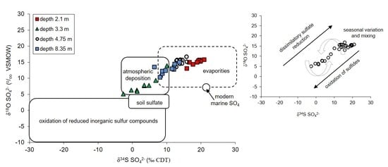
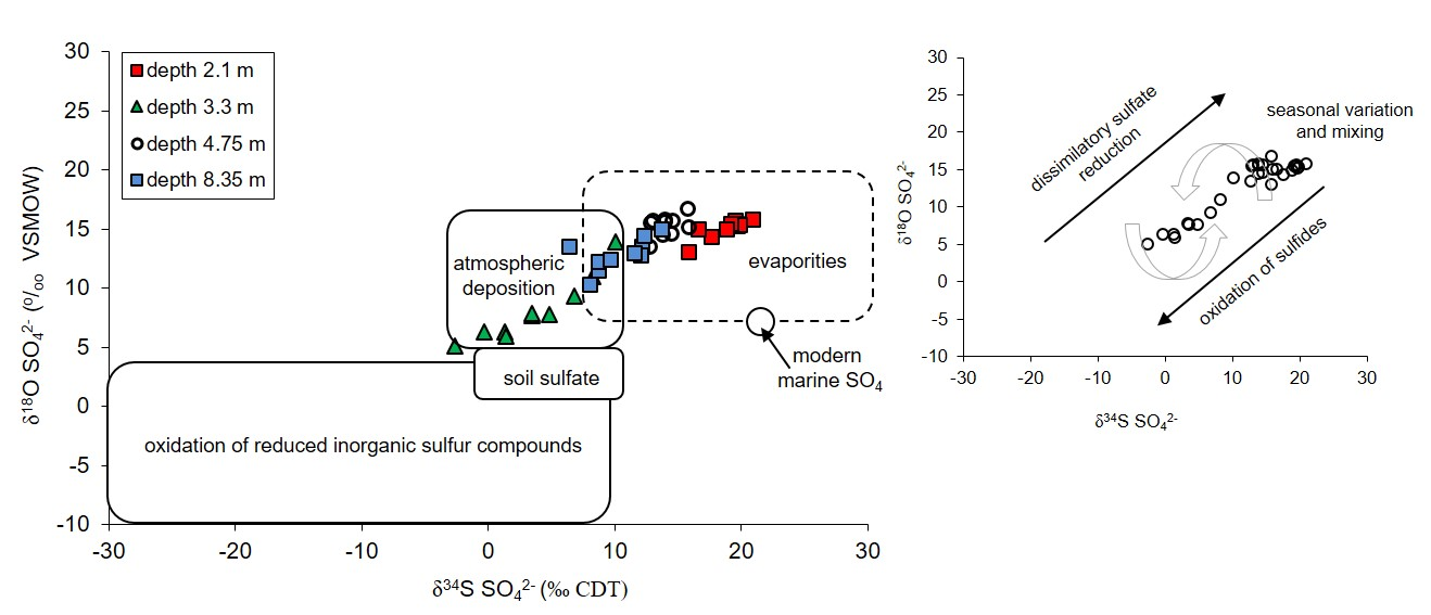
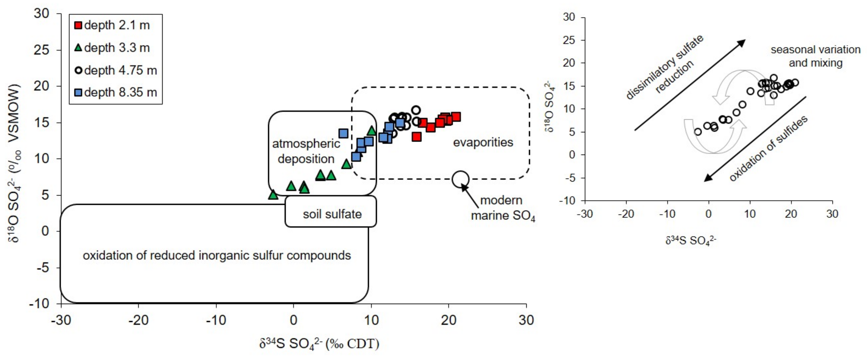
The atmospheric deposition—sulfates which are introduce to the aquifer with the recharge water such as rain and snowmelt. Their initial values of δ34SSO4 in the area of the Pożary research station documented for rain and snow varied from +4.3 to +8.8‰ with concentrations ranging from 1.7 to 14.2 mg/dm3. Such isotopic composition is typical for sulfate of anthropogenic origin in atmospheric precipitation in industrialized regions of the northern hemisphere with δ34S values ranging from −3 to +9‰. The atmospheric sulfates reach the aquifer by direct infiltration of recharging water though the peat layer and vadose zone and by lateral groundwater inflow from an adjacent areas, where the aquifer is not cover by peat.
(b)
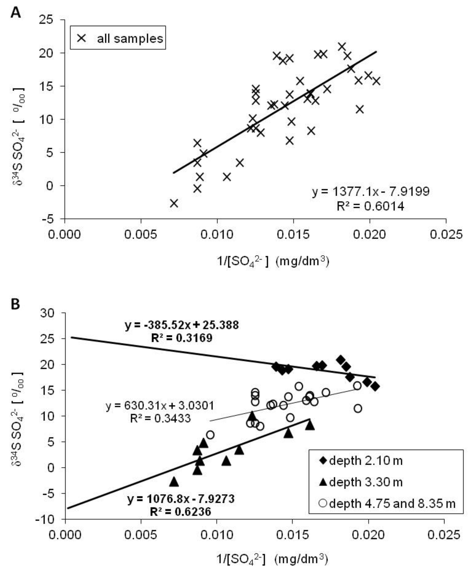
The evaporitic sulfate minerals (lithogenic source)—sulfates enriched in heavy 18O and 34S isotopes with δ34SSO4 ranging from +15.8 to +20.9‰ and δ18OSO4 from +13.0 to +15.8‰. Such isotopic composition is typical for sulfates originating most likely from the dissolution of evaporitic gypsum which may be formed in the peat layer or in the aquifer’s vadose zone during seasons with low groundwater level. Sulfates of such isotopic composition were observed exclusively in the most upper part of the aquifer profile (monitoring depth of 2.1 m) which is the closest to the overlying peat bed. It is very likely that the source of sulfates is connected with sulfate flax from the peat layer. Calculated initial value of the dominant source of dissolved sulfate at the depth of 2.1 m yielded a δ34SI value of +25.4‰, which also strongly suggests the influence of sulfates originating from bacterial sulfate reduction.
(c)
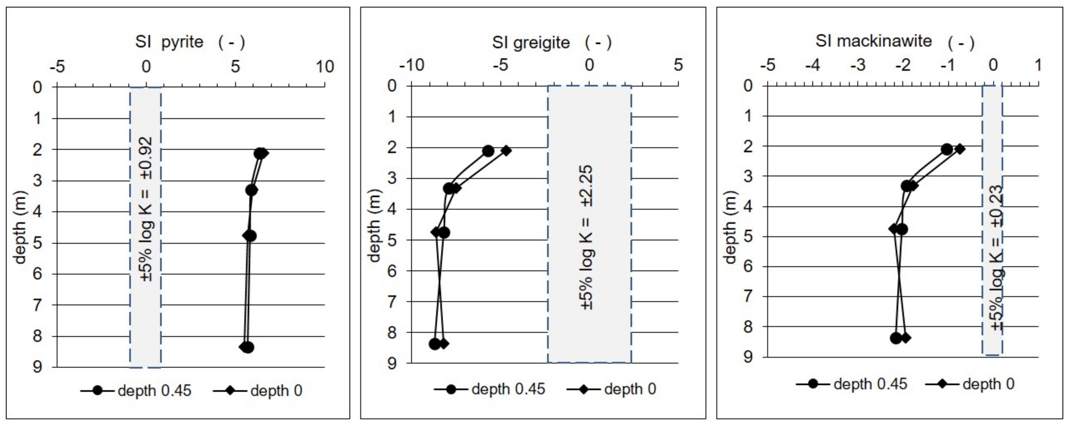
The reduced inorganic sulfur compound (RIS; lithogenic source)—sulfates depleted in heavy 18O and 34S isotopes with δ34SSO4 ranging from −2.6 to +10.1‰ and δ18OSO4—from +5.10 to +13.9‰. Sulfates of such isotopic composition were observed in the aquifer exclusively in monitoring depth of 3.3 m. Depletion in heavy isotopes is connected with increasing SO42− concentration: Usually increased from about 1.5–2 times (depending on the season) in relation to the uppermost part of the aquifer profile. The source of these sulfates is connected with oxidation/re-oxidation of reduced inorganic sulfur compounds in the aquifer i.e., first of all with the dissolution/precipitation of pyrite, the dissolution of greigite and mackinawite. Calculated initial value of the dominant source of dissolved sulfate at the depth of 3.3 m yielded a δ34SI value of −7.9‰ which corroborates that the oxidation of RIS is responsible for the increase in SO42− concentration in this part of the aquifer profile.
The observed linear trend of δ34S vs δ18O for aqueous sulfates can be attributed to (i) bacterial (dissimilatory) sulfate reduction, (ii) a mixing process in the aquifer, and/or (iii) the precipitation of sulfide minerals. Bacterial sulfate reduction is the most important biogeochemical process affecting the concentration and isotopic evolution of sulfates dissolved in groundwater in the Pożary aquifer.
The sulfur isotope enrichment factor (ε34S—expresses the partitioning magnitude of the 34S isotopes into the residual sulfates during bacterial sulfate reduction undergoing the Rayleigh fractionation model) calculated for each monitoring season revealed wide variation range from about −36.3 to −13.0‰. Such variation of ε34S corroborates that local climatic, environmental, and hydrogeological conditions have a strong impact on the bacterial sulfate reduction rate in the peat and in the aquifer, and on the final isotopic composition of the residual sulfates found in the studied groundwater. The highest absolute values of the enrichment factor ε34S are connected with seasons of decreasing vegetation activity (i.e., late autumn, winter, and early spring), lower ambient air temperature, and high levels of the groundwater table up to the ground surface (i.e., full saturation of the peat layer).
The bacterial sulfate reduction as a single process cannot fully explain the distribution of SO42− concentrations and the isotopic compositions of sulfur in the groundwater profile. The imposition of sulfide oxidation/re-oxidation, as well as groundwater mixing processes, must also be taken into account in the studied aquifer.
The biotic and abiotic transformations of sulfur compounds in the studied aquifer are interconnected with other geochemical processes through their common substrates or products. Bacterial sulfate reduction in groundwater profile results in change of isotopic signature of recharge water, a decrease of redox potential (Eh), slight decrease of pH, decrease of SO42−, increase of HCO3 (alkalinity), and precipitation of sulfide minerals. On the other hand, the imposition of the RIS oxidation causes the increase of water pH, the increase of SO42− concentration, and the decreases of alkalinity. The influence of this competitive processes of sulfur species transformations are reflected by the complex variations of the physicochemical parameters of groundwater and the concentration of chemical compounds across the aquifer profile. The monthly monitoring of the aquifer vertical profile allowed us to identify the zones where these different processes are dominant.
There are two issues that need further studies from the perspective of our experience gained during this research, namely, (i) the seasonal monitoring of the sulfate content and its isotopic composition inside the peat layer, and (ii) the identification and analysis of the main forms of the carbon-bonded sulfur compounds (C–S) in order to evaluate their influence on the formation of aqueous sulfates and sulfide minerals in groundwater in contacts with peatlands.

Author Contributions

Conceptualization, A.P. and D.P.; methodology, A.P.; software, A.P.; validation, S.H., D.P. and A.P.; formal analysis, S.H., A.P. and D.P.; investigation, A.P. and D.P.; data curation, D.P.; writing—original draft preparation, A.P. and D.P.; writing—review and editing, A.P.; visualization, D.P.

Funding

This research received funding in the framework of a joint statutory research task supported by the Institute of Geological Sciences of the Polish Academy of Sciences (INGPAN) and the Faculty of the Geology University of Warsaw. Part of the analytical studies was supported by the National Science Center Poland, grant No. UMO-2015/17/B/ST10/03295.

Acknowledgments

The authorities of the meteorological base station of Integrated Monitoring of the Natural Environment of the Kampinos National Park are thanked for their help in the collection of rainwater samples for chemical and isotopic analysis.

Conflicts of Interest

The authors declare no conflict of interest. The funders had no role in the design of the study; in the collection, analyses, or interpretation of data; in the writing of the manuscript, or in the decision to publish the results.

References

  1. Johnston, S.G.; Burton, E.D.; Aaso, T.; Tuckerman, G. Sulfur, iron and carbon cycling following hydrological restoration of acidic freshwater wetlands. Chem. Geol. 2014, 371, 9–26. [Google Scholar] [CrossRef]
  2. Langmuir, D. Aqueous Environmental Geochemistry; Prentice Hall: Upper Saddle River, NJ, USA, 1997; 600p. [Google Scholar]
  3. Appelo, C.A.J.; Postma, D. Geochemistry, Groundwater and Pollution; A.A. Balkema: Rotterdam, The Netherlands, 1996; 536p. [Google Scholar]
  4. Chapman, S.J. Sulfur forms in open and afforested areas of two Scottish peatlands. Water Air Soil Pollut. 2002, 128, 23–39. [Google Scholar] [CrossRef]
  5. Novak, M.; Vile, M.A.; Bottrell, S.H.; Stepanova, M.; Jackova, I.; Buzek, F.; Prechova, E.; Newton, R.J. Isotope systematic of sulfate-oxygen and sulfate-sulfur in six European peatlands. Biogeochemistry 2005, 76, 187–213. [Google Scholar] [CrossRef]
  6. López-Buendia, A.M.; Whateley, M.K.G.; Bastida, J.; Urquiola, M.M. Origins of mineral matter in peat marsh and peat bog deposits, Spain. Int. J. Coal Geol. 2007, 71, 246–262. [Google Scholar] [CrossRef]
  7. Alewell, C.; Paul, S.; Lischeid, G.; Storck, F.R. Co-regulation of redox processes in freshwater wetlansd as a function of organic matter availability? Sci. Total Environ. 2008, 404, 335–342. [Google Scholar] [CrossRef] [PubMed]
  8. Schwientek, M.; Einsiedl, F.; Stichler, W.; Stögbauer, A.; Strauss, H.; Maloszewski, P. Evidence for denitrification regulated by pyrite oxidation in heterogeneous porous groundwater system. Chem. Geol. 2008, 255, 60–67. [Google Scholar] [CrossRef]
  9. Wu, S.; Kuschk, P.; Wiessner, A.; Müller, J.; Sasd, R.A.B.; Dong, R. Sulphur transformations in constructed wetlands for wastewater treatment: A review. Ecol. Eng. 2013, 52, 278–289. [Google Scholar] [CrossRef]
  10. Wiessner, A.; Kappelmeyer, U.; Kuschk, P.; Kastner, M. Sulphate reduction and the removal of carbon and ammonia in a laboratory-scale constructed wetland. Water Res. 2005, 39, 4643–4650. [Google Scholar] [CrossRef]
  11. Schiff, S.L.; Spoelstra, J.; Semkin, R.G.; Jeffries, D.S. Drought induced pulses of from a Canadian shield wetland: use of δ34S and δ18O in to determine sources of sulfur. Appl. Geochem. 2005, 20, 691–700. [Google Scholar] [CrossRef]
  12. Clark, I.; Fritz, P. Environmental Isotopes in Hydrogeology; CRC Press LLC: Boca Raton, FL, USA, 1997; 328p. [Google Scholar]
  13. Mandernack, K.W.; Lynch, L.; Krouse, H.R.; Morgan, M.D. Sulfur cycling in wetland peat of the New Jersey Pinelands and its effect on stream water chemistry. Gechimica Cosmochiica Acta 2000, 64, 3949–3964. [Google Scholar] [CrossRef]
  14. Bottrell, S.H.; Hartfield, D.; Bartlett, R.; Spence, M.J.; Bartle, K.D.; Mortimer, R.J.G. Concentrations, sulfur isotopic compositions and origin of organosulfur compounds in pore waters of a highly polluted raised peatland. Org. Geochem. 2010, 41, 55–62. [Google Scholar] [CrossRef]
  15. Porowska, D.; Leśniak, P.M. Identification of processes controlling groundwater chemistry below peatland—Pożary, Kampinos Park Narodowy. Geol. Surv. 2008, 56, 982–990. (In Polish) [Google Scholar]
  16. Słowański, W.; Piechulska-Słowańska, B.; Gogołek, W. Geological Map of Poland in the Sacle 1:200 000. Warszawa-Zachód Sheet; PIG: Warszawa, Poland, 1994. [Google Scholar]
  17. Fic, M.; Wierzbicki, A. Organizacja sieci monitoringu wód podziemnych na terenie rezerwatu ”Pożary” w Kampinoskim Parku Narodowym. Geol. Surv. 1994, 42, 1004–1008. (In Polish) [Google Scholar]
  18. Ingram, H.A.P. Hydrology. In Mires, Swamps, Bog, Fen and Moore; Gore, A.J.P., Ed.; General Studies; Elsevier: Amsterdam, The Netherlands, 1983; Volume 4A, pp. 67–158. [Google Scholar]
  19. Witczak, S.; Kania, J.; Kmiecik, E. Katalog Wybranych Fizycznych i Chemicznych Wskaźników Zanieczyszczeń Wód Podziemnych i Metod ich Oznaczania; IOŚ: Warszawa, Poland, 2013; 648p. [Google Scholar]
  20. Nielsen, D.M.; Nielsen, G.L. The Essential Handbook of Ground-Water Sampling; CRC Press: Boca Raton, FL, USA, 2007; 309p. [Google Scholar]
  21. Weight, W.D.; Sonderegger, J.L. Manual of Applied Field Hydrogeology; McGraw-Hill: New York, NY, USA, 2000; 608p. [Google Scholar]
  22. Hermanowicz, W.; Dojlido, J.; Dożańska, W.; Koziorowski, B.; Zerbe, J. Fizyczno-Chemiczne Badanie Wody i ścieków; Wydawnictwo Arkady: Warszawa, Poland, 1999; 558p. (In Polish) [Google Scholar]
  23. Epstein, S.; Mayeda, T. Variation of 18O content of waters from natural sources. Geochim. Cosmochim. Acta 1953, 4, 213–224. [Google Scholar] [CrossRef]
  24. Roether, W. Water-CO2 set-up for routine 18Oxygene assay of natural waters. Int. J. Appl. Radiat. Isot. 1970, 21, 379–387. [Google Scholar] [CrossRef]
  25. Coleman, M.L.; Shepherd, T.J.; Durham, J.J.; Rouse, J.E.; Moore, G.R. Reduction of water with zinc for hydrogen isotope analysis. Anal. Chem. 1982, 54, 993–995. [Google Scholar] [CrossRef]
  26. Kendall, C.; Coplen, T.B. Multisample conversion of water to hydrogen by zinc for stable isotope determination. Anal. Chem. 1985, 57, 1437–1440. [Google Scholar] [CrossRef]
  27. Schimmelmann, A.; DeNiro, M.J. Preparation of organic and water hydrogen for stable isotope analysis: Effects due to reaction vessels and zinc reagent. Anal. Chem. 1993, 65, 789–792. [Google Scholar] [CrossRef]
  28. Porowski, A.; Kowski, P. Determination of δ2H and δ18O in saline oil-associated waters: the question of simple vacuum distillation of water samples prior to isotopic analyses. Isot. Environ. Health Stud. 2008, 44, 227–238. [Google Scholar] [CrossRef]
  29. Carmody, R.W.; Plummer, L.N.; Busenberg, E.; Coplen, T.B. Methods for Collection of Dissolved Sulfate and Sulfide and Analysis of Their Sulfur Isotopic Composition; U.S. Geological Survey Open-File Report; USGS Publication Warehouse: Reston, VA, USA, 1998; pp. 97–234.
  30. Mizutani, Y. An improvement in the carbon-reduction method for the oxygen isotopic analysis of sulphates. Geochem. J. 1971, 5, 69–77. [Google Scholar] [CrossRef]
  31. Halas, S.; Szaran, J.; Czarnacki, M.; Tanweer, A. Refinements in BaSO4 to CO2 preparation and δ18O-calibration of the sulphate standards NBS-127, IAEA SO-5 and IAEA SO-6. Geostand. Geoanal. Res. 2007, 31, 61–68. [Google Scholar] [CrossRef]
  32. Halas, S.; Szaran, J. Use of Cu2O-NaPO3 mixtures for SO2 extraction from BaSO4 for sulphur isotope analysis. Isot. Environ. Health Stud. 2004, 40, 229–231. [Google Scholar] [CrossRef] [PubMed]
  33. Porowska, D. Content of dissolved oxygen and carbon dioxide in groundwaters within the selected hydrogeocheical environment. Monogr. Kom. Gospod. Wodnej Pan 2004, 24, 137. [Google Scholar]
  34. Trudell, M.L.; Gillham, R.W.; Cherry, J.A. An in-situ study of the occurrence and rate of denitrification in a shallow unconfined sand aquifer. J. Hydrol. 1986, 86, 251–268. [Google Scholar] [CrossRef]
  35. Smith, R.L.; Duff, J.H. Denitrification in a sand and gravel aquifer. Appl. Environ. Microbiol. 1988, 54, 1071–1078. [Google Scholar] [PubMed]
  36. Böttcher, J.; Strebel, O.; Voerkelius, S.; Schmidt, H.L. Using isotope fractionation of nitrate nitrogen and nitrate oxygen for evaluation of denitrification in a sandy aquifer. J. Hydrol. 1990, 114, 413–424. [Google Scholar]
  37. Smith, R.L.; Howes, B.L.; Duff, L.H. Denitrification in nitrate-contaminated groundwater: occurrence in steep vertical geochemical gradients. Geochim. Cosmochim. Acta 1991, 55, 1815–1825. [Google Scholar] [CrossRef]
  38. Krogulec, E.; Jóźwiak, K. Mineral nitrogen in shallow waters of the Kampinos National Park. In Proceedings of the XII Sympozjum Współczesne Problemy Hydrogeologii, Kraków-Krynica, Poland, 21–23 June 2007; pp. 105–113. [Google Scholar]
  39. Krouse, H.R. Sulfur isotopes in our environment. In Handbook of Environmental Isotope Geochemistry. Volume 1: The Terrestrial Environment; Fritz, P., Fontes, J.C., Eds.; Elsevier: Amsterdam, The Netherlands, 1980; pp. 435–472. [Google Scholar]
  40. Krouse, H.R.; Mayer, B. Sulfur and oxygen isotopes in sulfate. In Environmental Tracers in Subsurface Hydrology; Cook, P., Herczeg, A.L., Eds.; Kluwer Academic Publishers: Dordrecht, The Netherlands, 2000; pp. 195–231. [Google Scholar]
  41. Knöller, K.; Fauville, A.; Mayer, B.; Strauch, G.; Friese, K.; Veizer, J. Sulfur cycling in an acid mining lake and its vicinity in Lusatia, Germany. Chem. Geol. 2004, 204, 303–323. [Google Scholar]
  42. Cook, P.G.; Herczeg, A.L. Environmental Tracers in Subsurface Hydrology; Kluwer: Boston, MA, USA, 2000; 529p. [Google Scholar]
  43. Porowski, A. Isotop hydrogeology. In Handbook of Engineering Hydrology. Volume 1. Fundamentals and Applications; Eslamian, S., Ed.; CRC Press: Boca Raton, FL, USA, 2014; pp. 345–378. [Google Scholar]
  44. Trembaczowski, A. Sulfur and oxygen isotopes behavior in sulfates of atmospheric groundwater system, observation and model. Nord. Hydrol. 1991, 22, 49–66. [Google Scholar] [CrossRef]
  45. Bottrell, S.H.; Coulson, J.; Spence, M.; Roworth, P.; Novak, M.; Forbes, L. Impacts of pollutant loading, climate variability and site management on the surface water quality of a lowland raised bog, Thorne Moors, E. England, UK. Appl. Geochem. 2004, 19, 413–422. [Google Scholar] [CrossRef]
  46. Skrzypek, G.; Akagi, T.; Drzewicki, W.; Jędrysek, M.O. Stable isotope studies of moss sulfur and sulfate from bog surface waters. Geochem. J. 2008, 42, 481–492. [Google Scholar] [CrossRef] [Green Version]
  47. Rozanski, K.; Araguas-Araguas, L.; Gonfiantini, R. Isotopic patterns in modern global precipitation. In Climate Change in Continental Isotopic Records. Geophysical Monograph; Stewart, P.K., Lohmann, K.C., McKenzie, J., Savin, S., Eds.; American Geophysical Union: Washington, DC, USA, 1993; pp. 1–36. [Google Scholar]
  48. Kroopnick, P.; Craig, H. Atmospheric oxygen: isotopic composition and solubility fractionation. Science 1972, 175, 54–55. [Google Scholar] [CrossRef] [PubMed]
  49. Everdingen, R.O.; Krouse, H.R. Isotope composition of sulphates generated by bacterial and abiological oxidation. Nature 1985, 315, 395–396. [Google Scholar] [CrossRef]
  50. Mayer, B.; Fritz, P.; Prietzel, J.; Krouse, H.R. The use of stable sulfur and oxygen isotope ratios for interpreting the mobility of sulfate in aerobic forest soils. Appl. Geochem. 1995, 10, 161–173. [Google Scholar] [CrossRef]
  51. Taylor, B.E.; Wheeler, M.C.; Nordstrom, D.K. Stable isotope geochemistry of acid mine drainage: experimental oxidation of pyrite. Geochim. Cosmochim. Acta 1984, 48, 2669–2678. [Google Scholar] [CrossRef]
  52. Porowska, D. Content of dissolved oxygen and carbon dioxide in rainwaters and groundwaters within the forest reserve of the Kampinos National Park and the urban area of Warsaw, Poland. Geol. Q. 2003, 47, 187–194. [Google Scholar]
  53. Rydelek, P. Origin and composition of mineral particles of selected peat deposits in Lubartowska Upland. Woda Śr. Obsz. Wiej. 2011, 11, 135–149. [Google Scholar]
  54. Mayer, B. Assessing sources and transformations of sulphate and nitrate in the hydrosphere using isotope techniques. In Isotopes in the Water Cycle; Past, Present and Future of a Developing Science; Aggarawal, P.K., Gat, J., Froehlich, K.F.O., Eds.; Springer: Dordrecht, The Netherlands, 2007; pp. 67–90. [Google Scholar]
  55. Zuber, A. Metody znacznikowe w badaniach hydrogeologicznych, poradnik metodyczny; Oficyna Wydawnicza Politechniki Wrocławskiej: Wrocław, Poland, 2007; 402p. (In Polish) [Google Scholar]
  56. Brown, K.A. Sulphur distribution and metabolism in waterlogged peat. Soil Biol. Biochem. 1985, 17, 39–45. [Google Scholar] [CrossRef]
  57. Rickard, D.; Luther, G.W., III. Chemistry of Iron Sulfides. Chem. Rev. 2007, 107, 514–562. [Google Scholar] [CrossRef]
  58. Rickard, D. Sulfidic Sediments and Sedimentary Rocks; Elsevier Science: Amsterdam, The Netherlands, 2012; Volume 65, 816p. [Google Scholar]
  59. Cohen, A.D.; Spackman, W. Methods in peat petrology and their application to reconstruction of paleoenvironments. Geol. Soc. Am. Bull. 1972, 83, 129–142. [Google Scholar] [CrossRef]
  60. Casagrande, D.J.; Seiffert, K.; Berschinski, C.; Sutton, N. Sulfur in peat forming systems of the Oekefenokee Swamp and Florida Everglades: origins of sulfur in coal. Geochim. Cosmochim. Acta 1977, 41, 161–167. [Google Scholar] [CrossRef]
  61. Philips, S.; Bustin, R.M. Sulfur in Changuinola peat deposit, Panama, as an indicator of the environments of deposition of peat and coal. J. Sediment. Res. 1996, 66, 184–196. [Google Scholar] [CrossRef]
  62. Berner, R.A.; Raiswell, R. Burial of organic carbon and pyrite sulfur ion sediments over Phanerozoic time: A new theory. Geochim. Cosmochim. Acta 1983, 47, 855–862. [Google Scholar] [CrossRef]
  63. Jóźwiak, K. Bogs iron ore in the marshy ground areas—e.g., Kampinoski National Park. Biul. Pig 2011, 445, 237–244. [Google Scholar]
  64. Wallace, A.; Wallace, G.A. Factors influencing oxidation of iron pyrite in soil. J. Plant Nutr. 1992, 15, 1579–1587. [Google Scholar] [CrossRef]
  65. Balci, N.; Shanks, W.C., III; Mayer, B.; Mandernack, K. Oxygen and sulfur isotope systematics of sulfate produced by bacterial and abiotic oxidation of pyrite. Geochim. Cosmochim. Acta 2007, 71, 3796–3811. [Google Scholar] [CrossRef]
  66. Canifeld, D.E. Isotope fractionation by natural populations of sulfate-reducing bacteria. Cosmochim. Acta 2001, 65, 1117–1124. [Google Scholar] [CrossRef]
  67. Samborska, K.; Halas, S. 34S and 18O in dissolved sulfate as tracers of hydrogeochemical evolution of the Triassic carbonate aquifer exposed to intense groundwater exploitation (Olkusz–Zawiercie region, southern Poland). Appl. Geochem. 2010, 25, 1397–1414. [Google Scholar] [CrossRef]
  68. Miao, Z.; Brusseau, M.L.; Carroll, K.C.; Carreón-Diazconti, C.; Johnson, B. Sulfate reduction in groundwater: characterization and applications for remediation. Environ. Geochem. Health 2012, 34, 539–550. [Google Scholar] [CrossRef]
  69. Kaplan, I.R.; Rittenberg, S.C. Microbiological fractionation of sulfur isotopes. J. Gen. Microbiol. 1964, 34, 195–212. [Google Scholar] [CrossRef]
  70. Rees, C.E. A steady-state model for sulfur isotope fractionation in bacterial reduction process. Geochim. Cosmochim. Acta 1973, 37, 1141–1162. [Google Scholar]
  71. Fritz, P.; Basharmal, G.M.; Drimmie, R.J.; Isen, J.; Qureshi, R.M. Oxygen isotope exchange between sulphate and water during bacterial sulfate reduction. Chem. Geol. 1989, 79, 99–105. [Google Scholar]
  72. Habicht, K.S.; Canfield, D.E. Sulfur isotope fractionation during bacterial sulfate reduction in organic-rich sediments. Geochim. Cosmochim. Acta 1997, 61, 5351–5361. [Google Scholar] [CrossRef]
  73. Mizutani, Y.; Rafter, T.A. Oxygen isotopic composition of sulphates, part 3: Oxygen isotopic fractionation in the bisulphate ion-water system. N. Z. J. Sci. 1969, 12, 54–59. [Google Scholar]
  74. Ahron, P.; Fu, B. Microbial sulfate reduction rates and sulfur and oxygen isotope ratios at oil and gas seeps in deepwater Gulf Mexico. Geochim. Cosmochim. Acta 2000, 64, 233–246. [Google Scholar] [CrossRef]
  75. Hoefs, J. Stable Isotope Geochemistry, 6th ed.; Springer: Berlin, Germany, 2009; 286p. [Google Scholar]
  76. Bottrell, S.H.; Smart, P.I.; Whitaker, F.; Raiswell, R. Geochemistry and isotope systematic of sulfur in the mixing zone of Bahamian blue holes. Appl. Geochem. 1991, 6, 97–103. [Google Scholar] [CrossRef]
  77. Bottrell, S.H.; Hayes, P.J.; Bannon, M.; Williams, G.M. Bacterial sulfate reduction and pyrite formation in a polluted sand aquifer. Geomicrobiol. J. 1995, 12, 75–90. [Google Scholar] [CrossRef]
  78. Bottrell, S.H.; Moncaster, S.M.; Tellam, J.H.; Lloyd, J.W.; Fisher, Q.J.; Newton, R.J. Control on bacterial sulfate reduction in a dual porosity aquifer system: The Lincoln Limestone aquifer, England. Chem. Geol. 2000, 169, 461–470. [Google Scholar] [CrossRef]
  79. Asmussen, G.; Strauch, G. Sulfate reduction in a lake and the groundwater of a former lignite mining area studied by stable sulfure and carbon isotopes. Water Air Soil Pollut. 1998, 108, 271–284. [Google Scholar] [CrossRef]
Figure 1. Location of the Pożary research station, geologic profile, and arrangement of piezometers for groundwater sampling. MS-KNP—meteorological station of Integrated Monitoring of the Natural Environment of the Kampinos National Park (KNP). Geological profile after Fic and Wierzbicki [17] modified by the authors.
Water 11 01388 g001
Figure 2. Seasonal variations of physicochemical parameters of groundwater in the Pożary aquifer vertical profile. The values for rainwater are shown at depth 0.0 m.
Water 11 01388 g002
Figure 3. Piper diagram showing chemical composition of groundwater in vertical profile of the Pożary aquifer. Rain water are plotted for reference. Archival records refer to groundwater monitoring period from June 1999 to December 2001 [15,33].
Water 11 01388 g003
Figure 4. Seasonal variations of chemical and isotopic composition of groundwater in the Pożary aquifer with depth. The values for rainwater are shown at depth 0.0 m. For more explanations see the text.
Water 11 01388 g004
Figure 5. The δ34S values and concentrations of dissolved sulfates in groundwater profile of the Pożary aquifer. For more explanations see the text.
Water 11 01388 g005
Figure 6. The δ2H vs. δ18O relationship in groundwater of the Pożary aquifer. Differentiation of isotopic composition is shown for sampling seasons (A) and depth profile (B). Global Meteoric Water Line (GMWL) after [47]: δ2H = 8.13 × δ18O + 10.8.
Water 11 01388 g006
Figure 7. Saturation indices (SI) with respect to gypsum calculated for chemical composition of water in two extreme positions of the groundwater level, namely: −0.45 m bgs in November 2009, and 0.0 m bgs (i.e., the groundwater level reaches the ground surface, the peat bed is fully saturated) in April 2010.
Water 11 01388 g007
Figure 8. Saturation indices (SI) with respect to pyrite, greigite, and mackinawite. Calculations were made for chemical composition of water in two extreme positions of groundwater level, i.e., −0.45 m bgs in November 2009, and 0.0 m bgs (i.e., the groundwater level reaches the ground surface, the peat bed is fully saturated) in April 2010.
Water 11 01388 g008
Figure 9. Trends of the δ34S and δ18O values for residual sulfates in groundwater of the Pożary aquifer. Linear correlations strongly suggest the occurrence of the bacterial sulfate reduction.
Water 11 01388 g009
Figure 10. Relationship between the fraction (f) of the residual sulfate and its δ34S and δ18O values in groundwater samples from the aquifer of the Pożary research station. Note: fraction f was calculated for modeling purpose.
Water 11 01388 g010
Figure 11. The δ34S versus δ18O of dissolved SO42− in groundwater of unconfined sandy aquifer against the background of typical sulfate sources and trends of biogeochemical processes.
Water 11 01388 g011
Table 1. Chemical composition of atmospheric precipitation and groundwater from piezometers in the Pożary research station. Rainwater is presented for depth 0.0 m. nd—not detected; na—not analyzed; <0.5—below detection limit.
DateDTpHEhSCCa2+Mg2+Na+K+HCO3SO42−ClNO3NH4+TDS
(m)(°C)(−)(mV)(uS/cm)(mg/dm3)
IX.2009rain105.87328523.90.41.42.18.66.13.30.62.328.7
2.110.17.06−28741124.021.211.21.2441.954.037.6<0.5na691.1
3.310.86.663151293.07.28.71.7172.062.058.3<0.5na402.9
4.7510.56.6823484102.012.29.60.2241.063.019.5<0.5na447.5
8.359.46.7425750138.08.49.71.0322.0105.040.8<0.5na624.9
X.2009rain9.55.74298443.00.41.10.8nd11.54.00.92.023.7
2.19.47.05−14758125.020.612.52.7431.855.135.5<0.5na683.2
3.39.56.833552196.711.68.91.7222.868.049.5<0.5na459.2
4.759.56.7126489104.612.19.10.2244.065.020.3<0.5na455.3
8.358.96.9723702116.012.79.80.8326.082.040.5<0.5na587.8
XI.2009rain105.65278454.10.51.00.4nd14.25.50.791.127.59
2.110.77.165752122.723.214.93.4416.260.450.5<0.5na691.3
3.39.26.8326528109.09.211.61.3199.687.260.5<0.5na478.4
4.759.66.731449998.98.59.40.2221.562.128.0<0.5na428.6
8.359.36.9324708135.512.34.30.6349.780.043.2<0.5na625.6
III.2010rain124.44257180.50.10.60.3nd2.13.50.671.08.77
2.113.17.149780130.025.911.91.4423.759.134.5<0.5na686.5
3.310.96.7873545101.08.08.80.3161.5113.252.9<0.5na445.7
4.7511.46.5684544103.08.312.10.2255.762.222.0<0.5na463.5
8.3512.46.89105749144.015.29.60.4374.969.560.1<0.5na673.7
VI.2010rain155.22315581.70.71.13.11.07.16.01.275.127.07
2.115.37.0960776129.027.515.20.9430.953.333.3<0.5na690.1
3.315.36.95106560104.08.111.50.2186.094.236.4<0.5na440.4
4.7514.56.65131591111.09.111.50.3277.058.229.7<0.5na496.8
8.3515.86.79100795149.015.913.00.3392.051.839.3<0.5na661.3
VII.2010rain165.59292351.30.20.51.31.14.74.00.601.815.5
2.115.77.0655759133.027.312.61.5420.650.329.3<0.5na674.6
3.317.26.9583542106.08.09.30.2198.681.439.0<0.5na442.5
4.7515.16.69109511104.08.18.30.2245.552.021.0<0.5na439.1
8.3516.16.8886731147.015.610.30.2383.067.448.4<0.5na671.9
Table 2. The isotopic composition of groundwater and dissolved sulfates in the Pożary aquifer at monitored depths throughout the observation period. na—not analyzed.
DateDδ18O H2Oδ2H H2Oδ18O SO4δ34S SO4SO42−DateDδ18O H2Oδ2H H2Oδ18O SO4δ34S SO4SO42−
(m)(‰) vs. VSMOW(‰) vs. VCDT(mg/dm3)(m)(‰) vs. VSMOW(‰) vs. VCDT(mg/dm3)
VIII.2009rain−7.48−55.4nana2.3II.2010snow−18.29−148.013.28.83.65
2.1−8.48−67.013.015.849.02.1−9.11−73.715.419.672.0
3.3−8.57−66.57.74.8110.03.3−8.45−68.17.83.4115.0
4.75−7.96−66.413.512.861.04.75−7.56−65.415.512.880.0
8.35−7.58−67.410.37.978.08.35−7.85−67.713.512.174.0
IX.2009rain−8.92−70.4Nana6.10III.2010rain−12.04−91.0nana2.1
2.1−9−67.215.719.554.02.1−9.08−73.315.419.859.1
3.3−8.45−65.711.08.362.03.3−8.33−68.86.31.4113.2
4.75−8.75−66.815.713.163.04.75−7.64−65.014.513.862.2
8.35−8.2−63.413.56.4105.08.35−7.7−66.412.812.169.5
X.2009rain−14.75−93.0Nana11.5IV.2010rain−10.42−77.8nanana
2.1−8.93−66.115.820.955.12.1−9.12−73.015.519.268.0
3.3−8.26−62.69.36.868.03.3−7.84−69.75.1−2.6140.0
4.75−8.64−64.616.815.765.04.75−7.47−64.915.613.980.0
8.35−8.4−65.111.58.782.08.35−6.76−61.114.512.373.0
XI.2009rain−11.03−87.9nana14.2V.2010rain−9.1−68.1nana2.1
2.1−9−73.015.319.760.42.1−9.03−73.915.018.870.0
3.3−8.29−68.17.73.587.23.3−7.95−67.86.3−0.4115.0
4.75−8.6−70.315.813.962.14.75−7.58−66.115.714.680.0
8.35−8.47−70.112.28.780.08.35−6.58−60.115.013.768.0
XII.2009snow−15.6−128.09.14.32.3VI.2010rain−5.64−40.29.86.07.1
2.1nanananana2.1−9.11−65.314.417.653.3
3.3nanananana3.3−7.93−58.95.91.494.2
4.75nanananana4.75−7.98−61.214.614.558.2
8.35nanananana8.35−6.94−55.612.9911.551.8
I.2010snow−15.67−124.9nana1.7VII.2010rain−8.17−63.5nana4.7
2.1nanananana2.1−9.17−65.715.116.650.3
3.3nanananana3.3−8.16−61.113.910.181.4
4.75nanananana4.75−8.88−65.315.115.952
8.35nanananana8.35−7.47−58.512.49.767.4

