Study on Pipe Burst Detection Frame Based on Water Distribution Model and Monitoring System

1
College of Civil Engineering and Architecture, Zhejiang University, Hangzhou 310058, China
2
Guangzhou Water Supply Co., Ltd., Guangzhou 510600, China
*
Author to whom correspondence should be addressed.
Water 2019, 11(7), 1363; https://doi.org/10.3390/w11071363
Submission received: 7 June 2019
/
Revised: 18 June 2019
/
Accepted: 25 June 2019
/
Published: 30 June 2019
(This article belongs to the Section Urban Water Management)
Abstract
:This paper describes an infrastructure to detect burst events in a water distribution network, which we illustrate using the Guangzhou water distribution system (WDS). We consider three issues: The feasibility and capability of accurate detection, the layout and design of the monitoring infrastructure, and the burst event detection algorithm. Background noise is identified by analyzing the monitored data. A burst event can be accurately detected only when the impact of the burst can be differentiated from the background noise. We hypothesize that there is a minimum pipe diameter below which accurate burst detection is impossible. We found that data from at least two sensors close to the burst event are required to reduce detection errors.
1. Introduction
Pipe burst events are widespread in water distribution systems (WDS). Detection of pipe burst events has usually been by direct visual observation or customer reports. These methods are time-consuming and are not reliable. Water companies must locate burst events quickly and accurately to reduce water loss and damage from pipe bursts, such as water waste, secondary pollution, and real estate damage. Various techniques have been devised to detect burst events. These techniques can be broadly divided into equipment-based methods and software-based methods [1].
Equipment-based methods use hardware (e.g., listening sticks, leak noise correlators, vibro-acoustic techniques, gas injection techniques, ground penetrating radar) to detect and locate bursts. These techniques are effective and fairly accurate. However, their use is limited by financial costs and detection time, and their accuracy is usually biased by worker experience.
Software methods have been important in burst detection since they were introduced in the 1990s. Transient detection methods use pressure wave signals for burst detection. These methods include transient analysis, inverse transient analysis, and time-frequency domain analysis. To find leaks, Pudar and Liggett [2] developed a method of inverse analysis based on water pressure, and they suggested it be used to supplement traditional leak detection methods. Vítkovský et al. [3] used a Levenberge–Marquardt algorithm to estimate the magnitude and location of a single leak in a pipeline. This method is also suitable for situations where there are two or more leaks. Misiunas [4] continuously monitored a laboratory pipeline for pressure transients to detect and locate burst events; the method can be used in an operational pipeline system. Kapelan et al. [5] created an inverse transient model to detect leaks. They calibrated pipe roughness by incorporating parameterized prior information and found that the use of prior information improved the results given by the model. Lee [6] devised a frequency domain method to locate a burst event. This method determines the exact location and magnitude of one or more leaks using frequency response curve. Methods using fluid transients can analyze the hydraulic behavior of the WDSs for burst detection. However, they require a lot of data, which are very expensive to collect, and these methods lack enough field trials for adequate validation.
Other software-based methods, such as statistical and artificial intelligence methods, have been widely used as hydraulic models, and data analysis techniques have been developed. These methods are promising and have recently become more popular as they can extract burst-related information from large amounts of data to identify bursts. Mounce and Machell [7] found a relationship between pipe burst events and fluctuations in pressure and flow by using artificial neural networks (ANNs). The results show that both static and time-delayed ANNs can identify bursts, and the effectiveness of the ANN is determined by the quantity and quality of data. Bicik [8] used Dempster–Shafer (D-S) evidence theory, which combines the outputs of different models, to provide increased confidence in the results of individual models and rapidly localize bursts. Cheng et al. [9] also used D-S theory combined with pressure and flow risk functions to identify bursts on a water main trunk. A burst detection system was built using this method and correctly identified all bursts from one-year historical records. Ye and Fenner [10] developed an adaptive Kalman filter for flow and pressure observations at a district meter area to detect burst events. The burst events that were detected matched observed events, and the authors used the pressure-based detection method to confirm the flow-based method. Jung and Lancey [11] developed a nonlinear Kalman filter which was robust in a variety of operations to detect burst events. Palau et al. [12] identified anomalous behaviors in water use, burst events, and illegal connections using principal component analysis. This method was very sensitive in detecting bursts and other abnormal events. Romano et al. [13] developed an event recognition system (ERS) for automated burst detection using statistical and artificial intelligence techniques. Several cases showed that the ERS can detect burst events quickly and reliably. Jung et al. [14] compared six statistical process control methods in terms of burst detection capability and found that an exponentially weighted moving average method was the most reliable. Besides, the method had the shortest detection time. However, these methods that use data mining have a high false alarm rate because they could be affected by uncertainty in the monitored data, which makes their widespread use impractical.
Burst detection methods and algorithms have been extensively and thoroughly studied, and progress has been made in recent years. In this paper, our focus is not on a new burst identification method. Instead, we introduce a burst detection process that explores the impact of a simulated burst event on the WDS and the reduction of the false alarm rate of the current monitoring system. This paper details two aspects of our work. First, the method of determining the background noise, using observed data from supervisory control and data acquisition (SCADA), is described. A burst event can be accurately detected only when the impact of the burst can be differentiated from the background noise. Based on this assumption, the threshold for burst detection and the minimum pipe diameter for which a burst event is detectable can be determined for any given WDS. Second, the method of determining the minimum number of sensors is described. This determination will improve the acceptability rate of correctly detected burst events.
The rest of this paper is organized as follows. The main requirements for building a comprehensive burst detection system are described in Section 2. In Section 3, we estimate the level of background noise in the data that have been collected and determine the thresholds of pressure that identify abnormal fluctuation from the cumulative probabilities of pressure fluctuations and head loss fluctuations. In Section 4, we define the minimum pipe diameter for which a burst event is detectable; that is, when burst event data are discernible from background noise. Only burst events in sufficiently large diameter pipes would cause a noticeable pressure drop. Finally, we identify the number of sensors required to determine a burst location by analyzing burst records collected over one year and suggest a simple burst detection method by comparing pressure drop and threshold values in Section 5. The main conclusions are given in Section 6.
2. Framework of the Burst Detection System
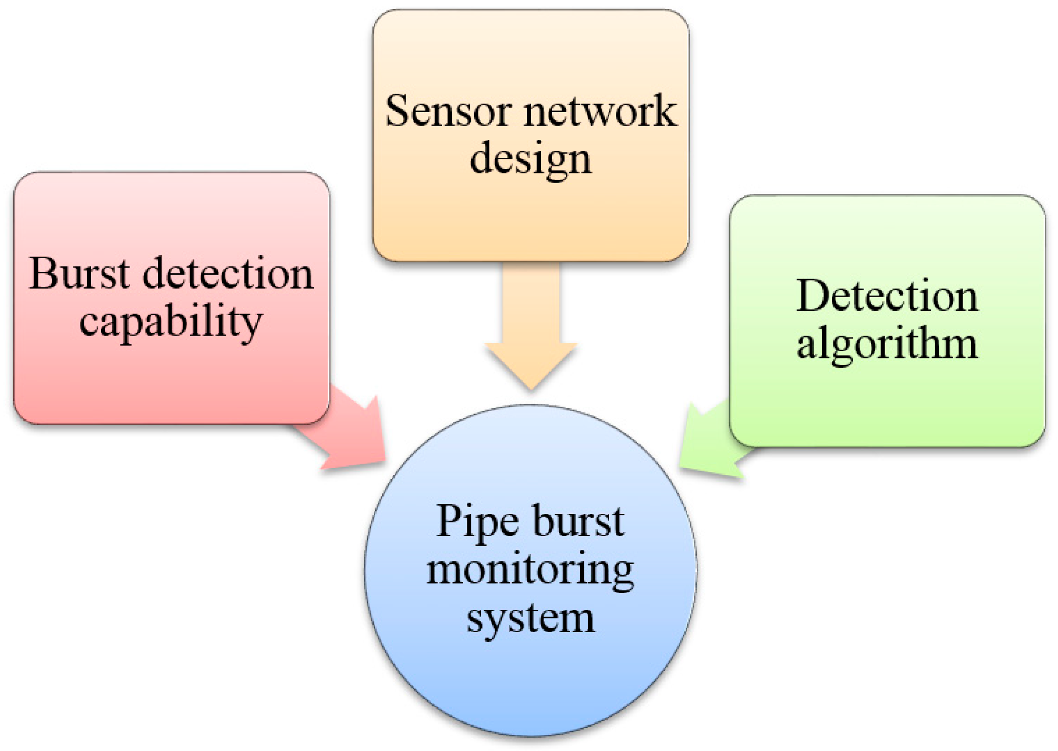
Before creating a burst detection system, three issues must be addressed (Figure 1):
- (1)
- Burst detection capability: What is the minimum burst that the monitoring system can detect? For example, a burst in a 1200 mm diameter pipe may easily be detected whereas a burst in a 50 mm diameter pipe may be undetected. Specifically, what pipe diameter is the minimum for burst events to be detectable?
- (2)
- Sensor network design: How many pressure sensors and flow meters are needed, and where should they be installed?
- (3)
- Detection algorithm: How do we analyze the monitoring data and determine the probability that a burst event has occurred?
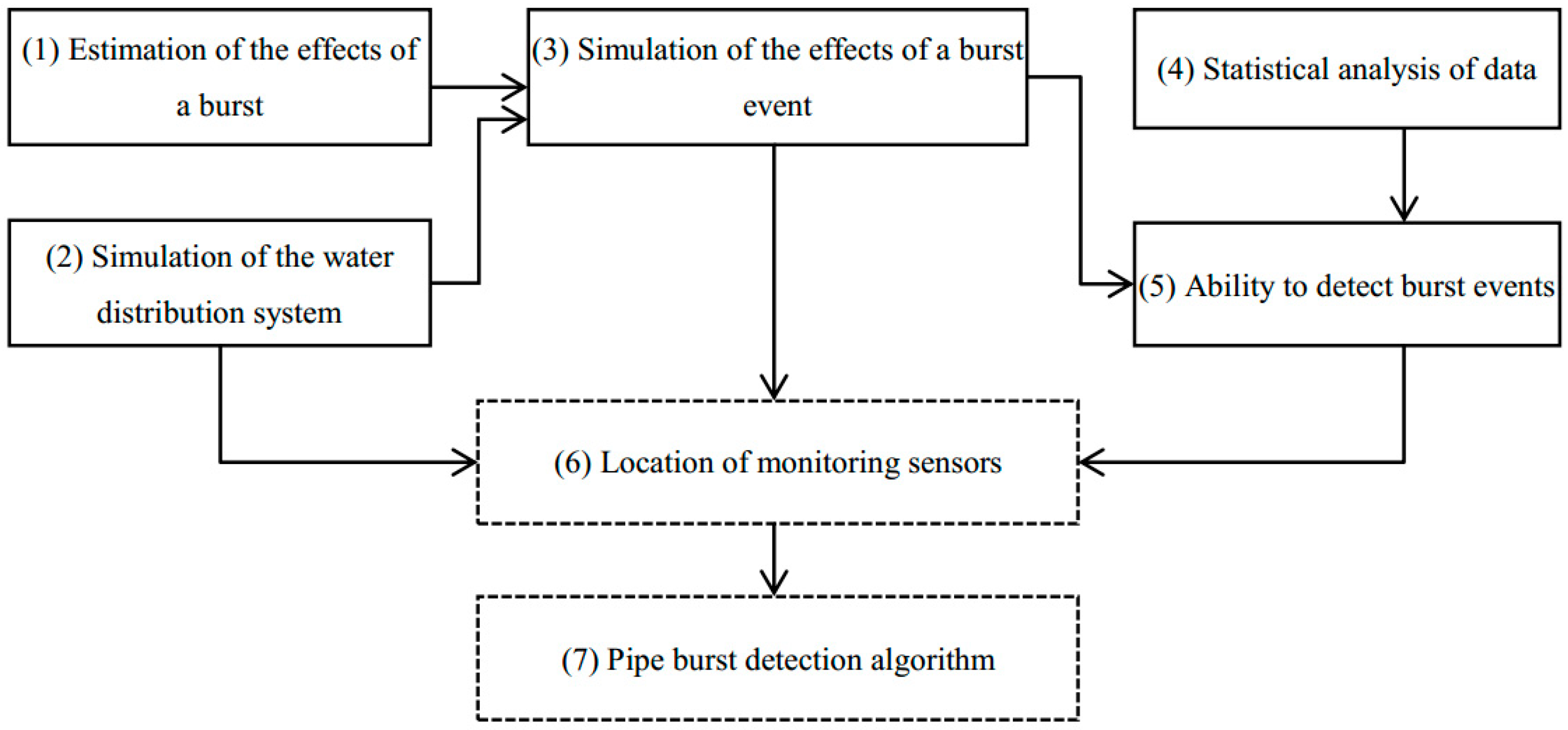
A flowchart for creating a monitoring system to detect burst events that is aligned with these three principles is shown in Figure 2. A brief description of each of the seven components follows:
- Estimation of the effects of a burst: When a burst event occurs, how much flow will be lost through the leak?
- Simulation of the water distribution system: A quantitative hydraulic model is used to represent the WDS.
- Simulation of the effects of a burst event: A pipe burst is a random event that may occur anywhere and anytime. The WDS model should predict the probable impact of a pipe burst.
- Statistical analysis of data: A WDS is dynamic; there are periodic patterns in its operation; and its periodic pressure and flow can be easily monitored. However, water consumption changes randomly, causing synchronous fluctuations in pressure and flow. Electromagnetic interference may also randomly distort monitoring data and create background noise. Hence, recognizing the statistical characteristics of data and background noise help to identify abnormal events.
- Ability to detect burst events: Few instruments can measure the water loss from a leak in a 15 mm pipe because the flow is so small that the impact of a leak will be seen as background noise. This leads to an interesting question (discussed in Section 4.2): What is the minimum diameter of pipe for which a burst event can be accurately detected (minimum detectable diameter of pipe burst, MDDPB).
- Location of monitoring sensors: The placement of sensors in a WDS is widely debated, and they can be used for different purposes, such as burst detection, contamination detection, and model calibration [15,16]. Sensor placement can be optimized by using multi-objective models. In this paper, the purpose of the monitoring network is to detect burst events.
- Pipe burst detection algorithm: There is no consensus concerning the best algorithm. Any algorithm used in modelling a WDS should be validated against real burst events. An ideal algorithm will be 100% accurate: it will detect all leaks that do occur and will not falsely detect leaks that have not occurred. An effective algorithm will be close to ideal.
Boxes 1 to 5 in Figure 2 address the first issue, and boxes 6 and 7 address the second and third issues. In this paper, we focus on the first issue, the feasibility and capability of accurately detecting burst events. We have carried out research in estimating the flow in a burst pipe, box 1 [17], in which the flow coefficient is estimated according to the size of the burst and the incoming water velocity. In the rest of this paper, we discuss boxes 4 and 5 which use the observed data.
3. Statistical Characteristics of Observed Data
Supervisory control and data acquisition (SCADA) infrastructure is used by water companies to detect pipe burst events. Flow and pressure data are sent to a control center via a general packet radio service (GPRS) every 5–15 min. In this section, we use data observed at Guangzhou over one year for statistical analysis.
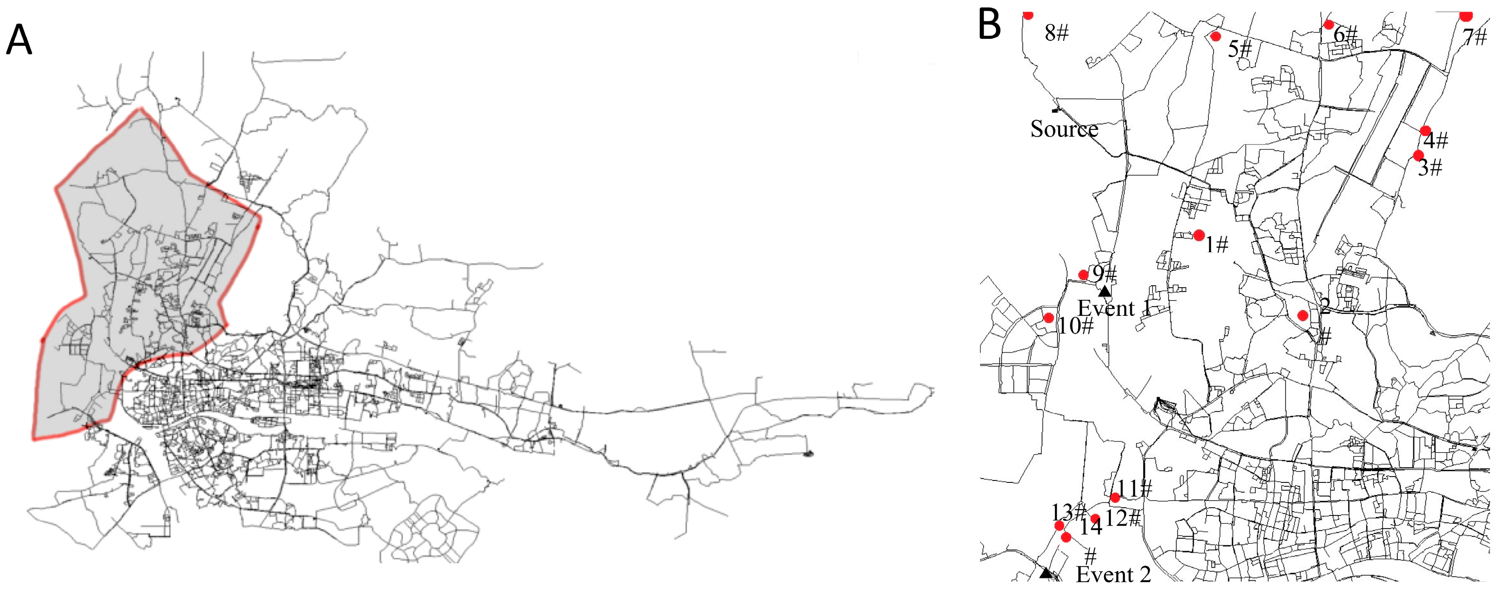
Guangzhou’s WDS is one of the largest systems in China. It has seven water reservoirs and supplies 400 million m3/d water. The study area is supplied by the Shimen water plant (Figure 3A). Fourteen pressure sensors are installed in the area, denoted by the numbers 1#–14# in Figure 3B.
3.1. Pressure Fluctuation in WDS
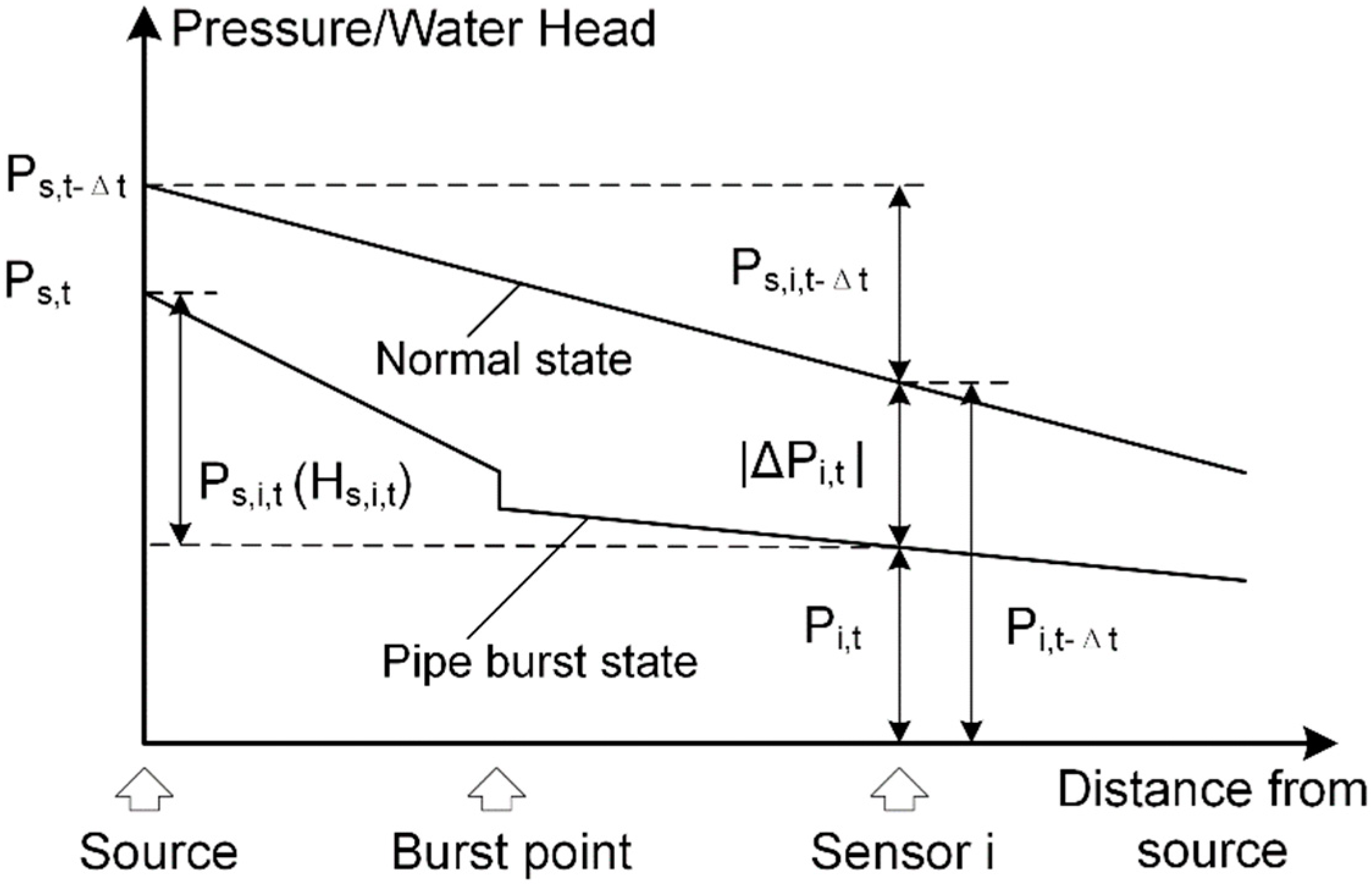
The state change of a pipe after a burst event is shown in Figure 4, where Pi,t is the pressure monitored by sensor i at time t. Ps,t and Qs,t are reservoir pressure and flow. Pressure fluctuation at sensor i at time t is:
Head loss from the reservoir to the sensor i is:
where Zs and Zi are the elevations at the reservoir and at sensor i. Because Zs − Zi is constant for the two nodes, the head loss fluctuation ΔHs,i,t is equal to ΔPs,i,t:
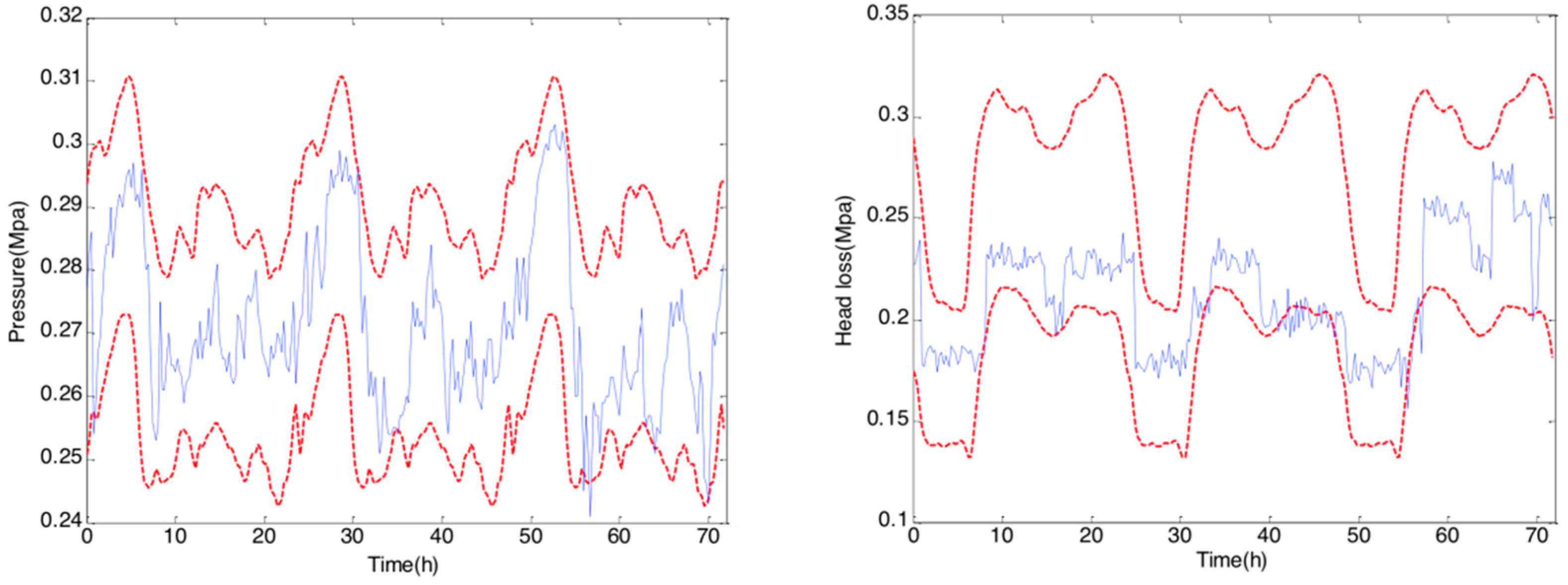
When water consumption increases abruptly or a burst event occurs, the pressure drops and the head loss increases, expressed as ΔPi,t < 0 and ΔPs,i,t > 0. As water consumption is a random variable, the pressure and head losses fluctuate over a wide range (Figure 5). However, ΔPi,t < 0 and ΔPs,i,t > 0 does not imply with certainty that a burst event has occurred. It is necessary to establish a suitable criterion to determine the abnormal events.
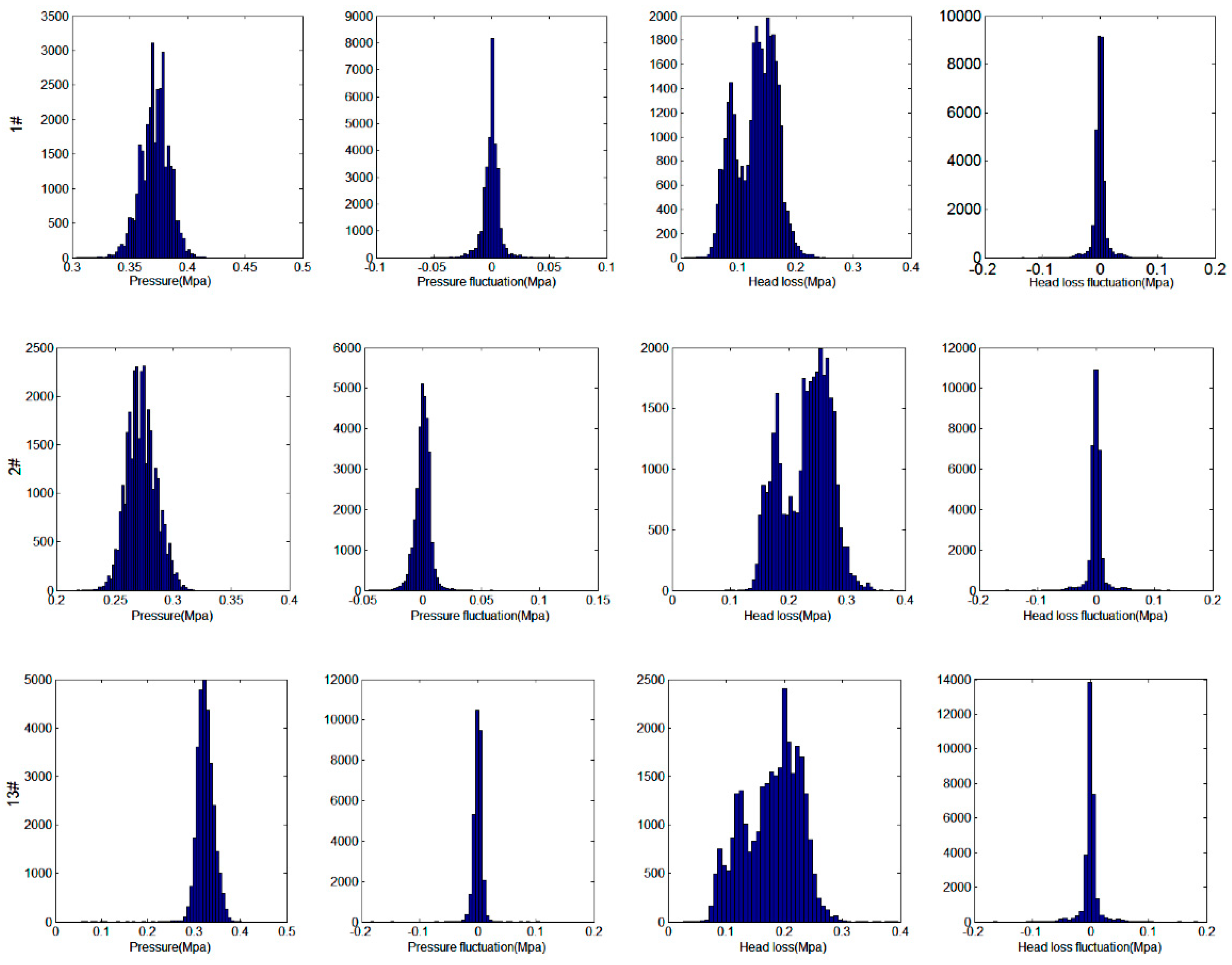
Histograms of the data from three sensors (1#, 2#, and 13#) are shown in Figure 6. The first histogram is pressure distribution, the second is pressure fluctuation, the third is head loss, and the fourth is head loss fluctuation. The third histogram shows that head loss Hs,i,t has a multimodal distribution. Pressure fluctuation ΔPi,t and pressure loss fluctuation ΔPs,i,t (ΔHs,i,t) are unimodal and show an approximately normal distribution.
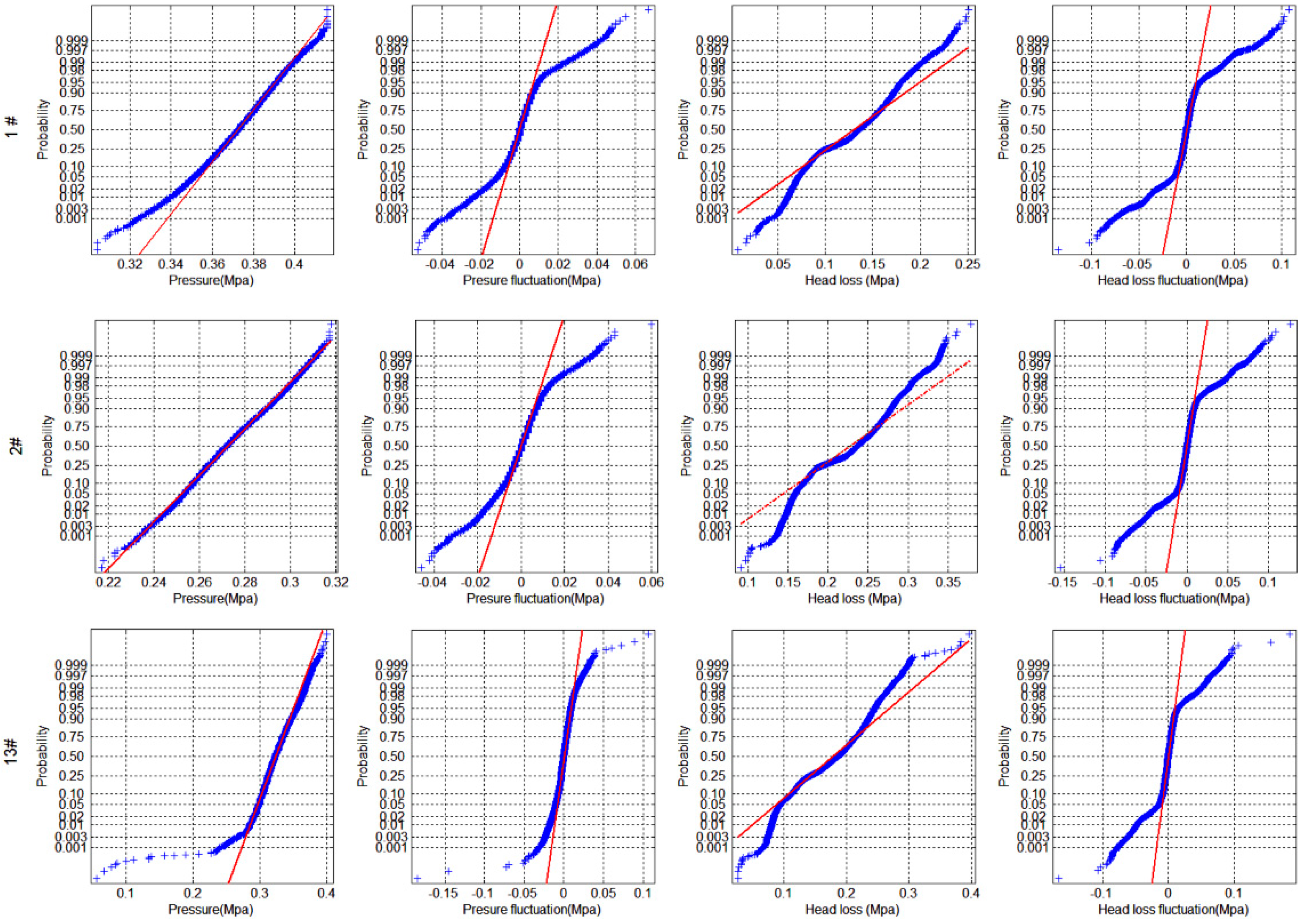
The cumulative probability distribution curves are shown in Figure 7. Straight red lines are the theoretical cumulative normal probability distributions (normal distribution error function); blue plus symbols are the observed cumulative probability distributions. We see that ΔPi,t is close to the normal distribution within the probability range 0.1–0.95. The empirical value is less than the theoretical value when the cumulative probability is <0.05. It is greater than the theoretical value when the cumulative probability is >0.95. The head loss fluctuation ΔPs,i,t shows distributions similar to ΔPi,t.
3.2. Thresholds of Abnormal Pressure Fluctuation
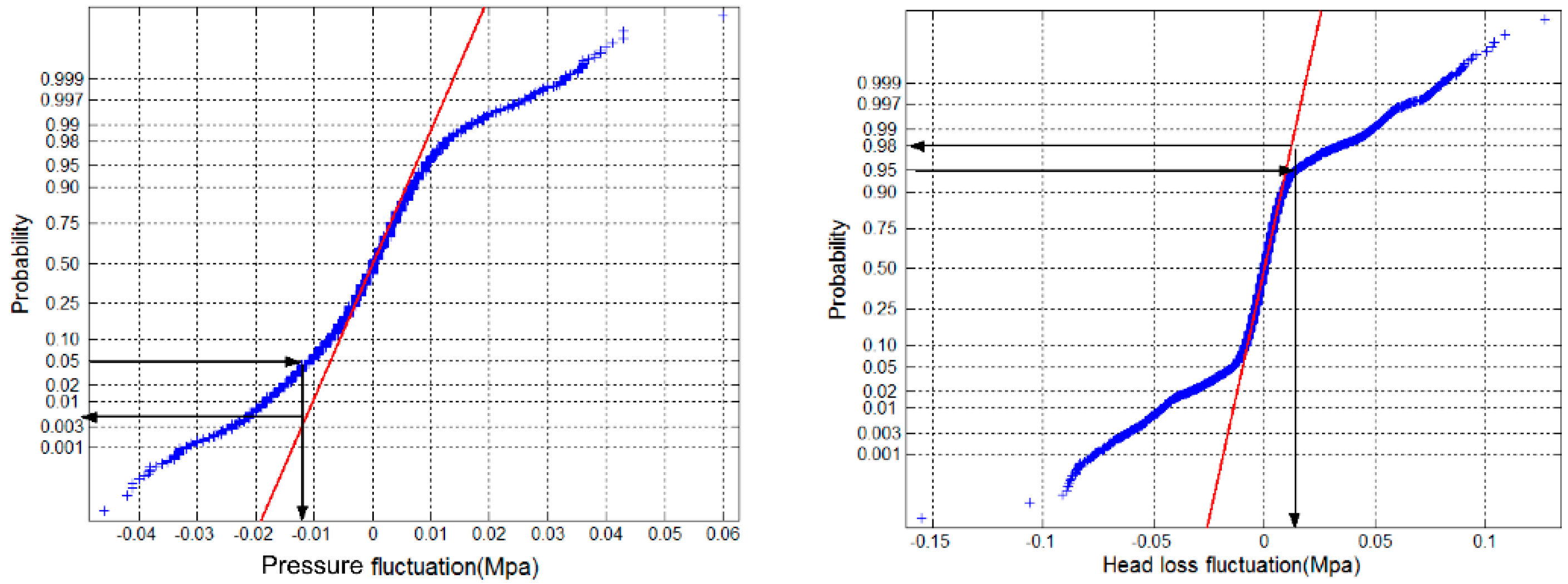
The empirical three-sigma rule of a normal distribution is widely used to identify abnormal data. Figure 8 shows that the cumulative probability distributions deviate from the cumulative normal distributions when the cumulative probability is <5% or >95%. The inflection on the cumulative probability distribution can be set as the threshold value for identifying an abnormal event, which is just 2–3 standard deviations.
When the pressure drop ΔPi,t is <0, a larger absolute value indicates a greater probability of an abnormal event. In the cumulative probability distribution of observed pressure fluctuations, the point with probability 5% can be defined as the key point, and the corresponding pressure drop is the threshold (). The head loss will increase after the burst event. The point on the cumulative probability distribution of observed head loss fluctuation with probability 95% is the key point, and its head loss increment is the threshold (). Figure 8 shows the determination of and for sensor 2. When the pressure falls below the threshold value or head loss fluctuations exceed the threshold value, abnormal events may be indicated.
A burst event is a rare occurrence. Figure 8 shows that if data (ΔPi,t and ΔPs,i,t) from one sensor exceed thresholds, there is a 95% probability of it being an abnormal event. The false alarm rate is 5%, which is relatively high. If two sensors both exceed the thresholds, the false alarm rate can be greatly reduced to 0.25% (5% × 5%). Therefore, we need to determine the minimum number of sensors in a detection zone (i.e., the part of the network close to and containing the burst event) for an acceptable rate of correctly detected burst events. This will be discussed in Section 5.2.
4. Impact of Burst Events on WDS
4.1. Simulation of Burst Event
A pipe burst event affects both the pressure and flow of a WDS. The effects depend on the structure of the WDS, the level of damage to the pipes, and the pipe diameters. A burst event causing a certain degree of damage at a particular pressure usually has greater impact on a DN1200 mm pipe than it would on a DN600 mm pipe. Thus, it is easier to detect the DN1200 mm pipe burst. It is difficult to directly measure the effects of a pipe burst event on a WDS. The hydraulic model provides a means of evaluating the effects. The following sections describe a method of modeling and evaluating the impact of a simulated burst event and an analysis of the minimum pipe diameter for detection of a burst event.
EPANET provides a pressure-dependent jet flow model, which can simulate a burst event by setting the emitter coefficient. The jet flow function is:
where C is the emitter coefficient, HL is the pressure at the leak point, and QL is the leak flow C can be expressed as:
where μ is the discharge coefficient and is related to the pressure, the incoming velocity, and the shape of the hole. According to our previous research [17], we set μ = 0.4, and C is given by:
where AL is the area of the hole (m2), AD is the area of the pipe cross-section, and n represents the ratio of hole area to pipe cross-section area. In this study, n ranges from 2 to 1/32, with a typical value being 1/2. In the following simulations, we assume that burst events occur close to sensors 1#, 9#, and 10# and the adjacent pipes are DN1200 mm, DN800 mm, DN600 mm, DN400 mm, and DN300 mm.
4.2. Minimum Pipe Diameter for Burst Detection
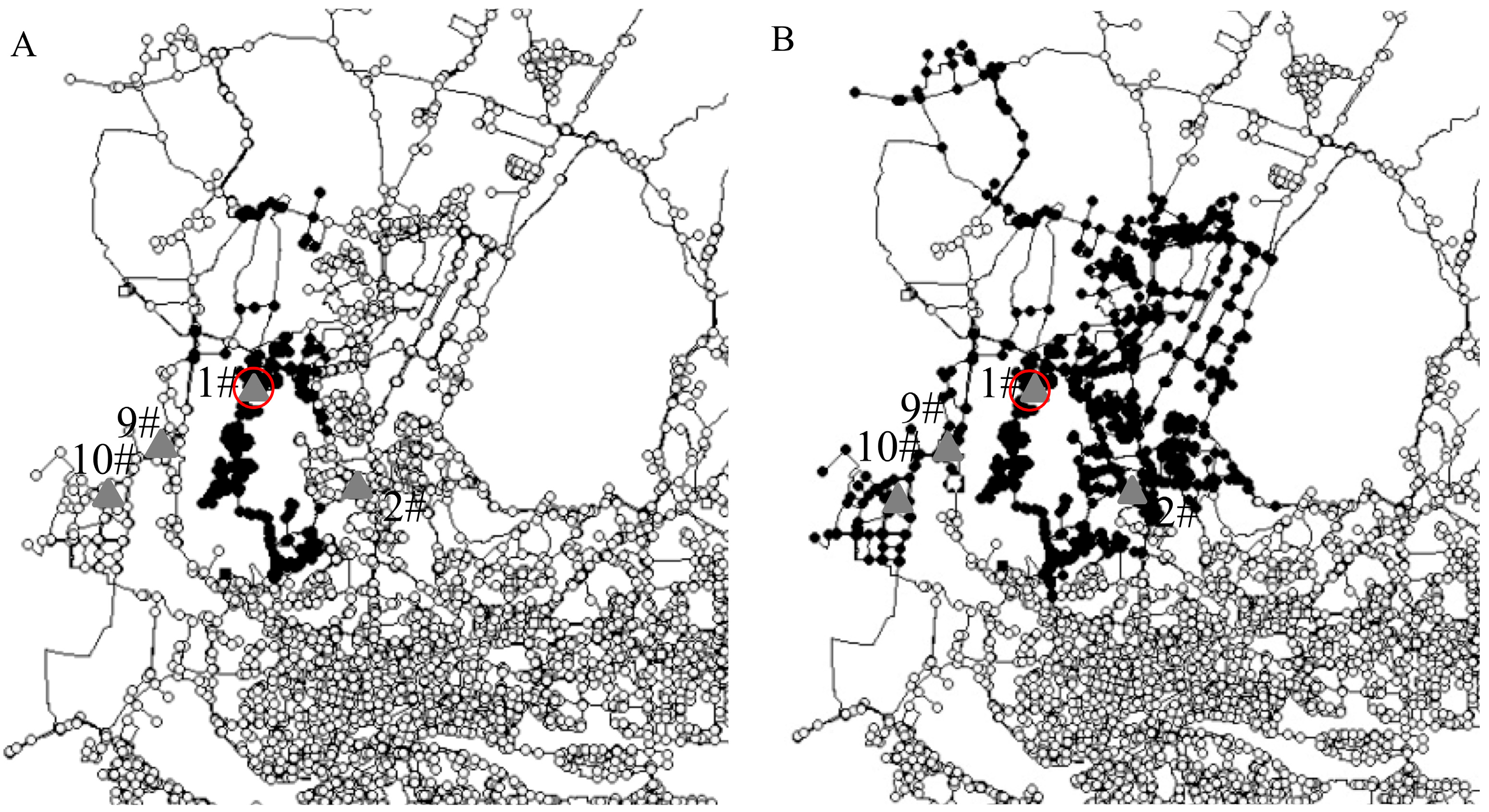
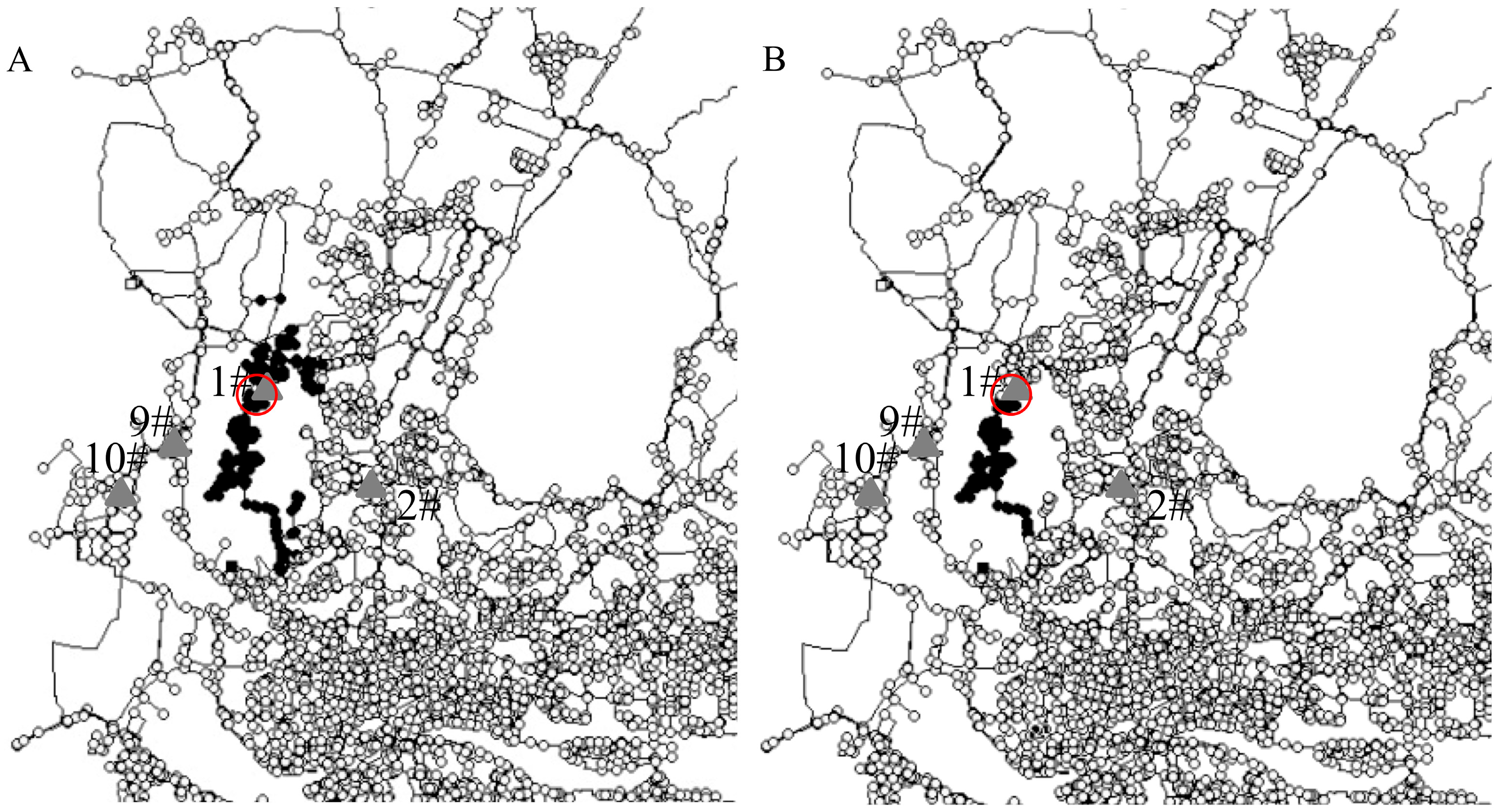
The pressure drop due to a burst event is calculated by the model of the WDS. Nodes at which the pressure drop is greater than the average threshold value are shown by the model as black dots (Figure 9 and Figure 10).
Table 1 shows the pressure drop at sensors 1#, 9#, and 10# and the burst event nodes (or points, BEP*) for different pipe diameters, with different values of n and corresponding values of C. When the burst pipe diameter is 1200 mm, most of the pressure drop values at the sensor are greater than the average Δ (i = 1, 9, 10), even for n = 1/8. Figure 9A shows that the black dots are metered by two pressure sensors. This means that, because bursts can be easily identified by the sensors, most bursts in 1200 mm diameter pipes are detectable.
Figure 9B shows that the black dots (nodes at which the pressure drop is greater than the average threshold value) are metered by three sensors when there is a burst event in a DN800 pipe with n = 1/2, which means that the DN800 mm burst is detectable in this case. Figure 10A shows the pressure drop of a DN600 mm pipe with n = 1/2. There are fewer black dots, but two sensors show a pressure drop greater than the threshold value. We conclude that the burst is detectable when the pipe diameter is 600 mm. When the burst pipe diameter is 400 mm (Figure 10B) or 300 mm, most sensors show pressure drops that are , even with n = 1 or 2. This means that it is difficult to detect bursts in pipes with diameter <400 mm. From Figure 9 and Figure 10, and Table 1, we conclude that the minimum diameter of pipes in Guangzhou for which leaks are detectable is 600 mm.
5. Pipe Burst Detection
5.1. Pipe Burst Event
A simple burst detection method is to compare the pressure drop and head loss at a sensor with the threshold values. If the pressure drop and head loss both exceed the threshold values, a burst may occur near this sensor. We use a case in Guangzhou to validate the model.
A pipe burst event occurred at 13 Februrary 2010 22:15 (Figure 3B, Event 1). The burst pipe diameter is 1800 mm. When the event occurred, pressure at the pump station decreased by 0.59 m, and the flow increased by 560 m3/h (5% of total flow). However, it is difficult to determine that a burst event occurred from the data for the observed pressure drop and flow increase. We use the thresholds method mentioned in Section 3.2 for further determination. The threshold values (ΔPc i,t and ΔPc s,i,t) of all sensors are calculated, as shown in Table 2. The average value of ΔPc i,t is −1.24 m and the average value of ΔPc s,i,t is 1.57 m.
The variations of pressure (ΔPi,t) and head loss (ΔPs,i,t) after the burst are shown in Table 3. When ΔPs,i,t and ΔPi,t exceed the average threshold values, it is shown as 1 in the fifth row of the table, otherwise 0. Sensors 1#, 2#, 5#, 8#, 9#, 10#, 11#, 12#, and 13# are l. Among them, sensors 9#, 10#, 1#, and 2# have the four greatest ΔPs,i,t values. However, sensor 2# is located far away from the other sensors, so it is excluded. The most probable location of the pipe burst is somewhere near sensors 9#, 10#, and 1#. The monitoring records show that the burst location (Event 1) was really near sensor 9#, which shows this method is feasible for detecting and locating bursts.
5.2. Suggested Sensor Numbers for Burst Detection
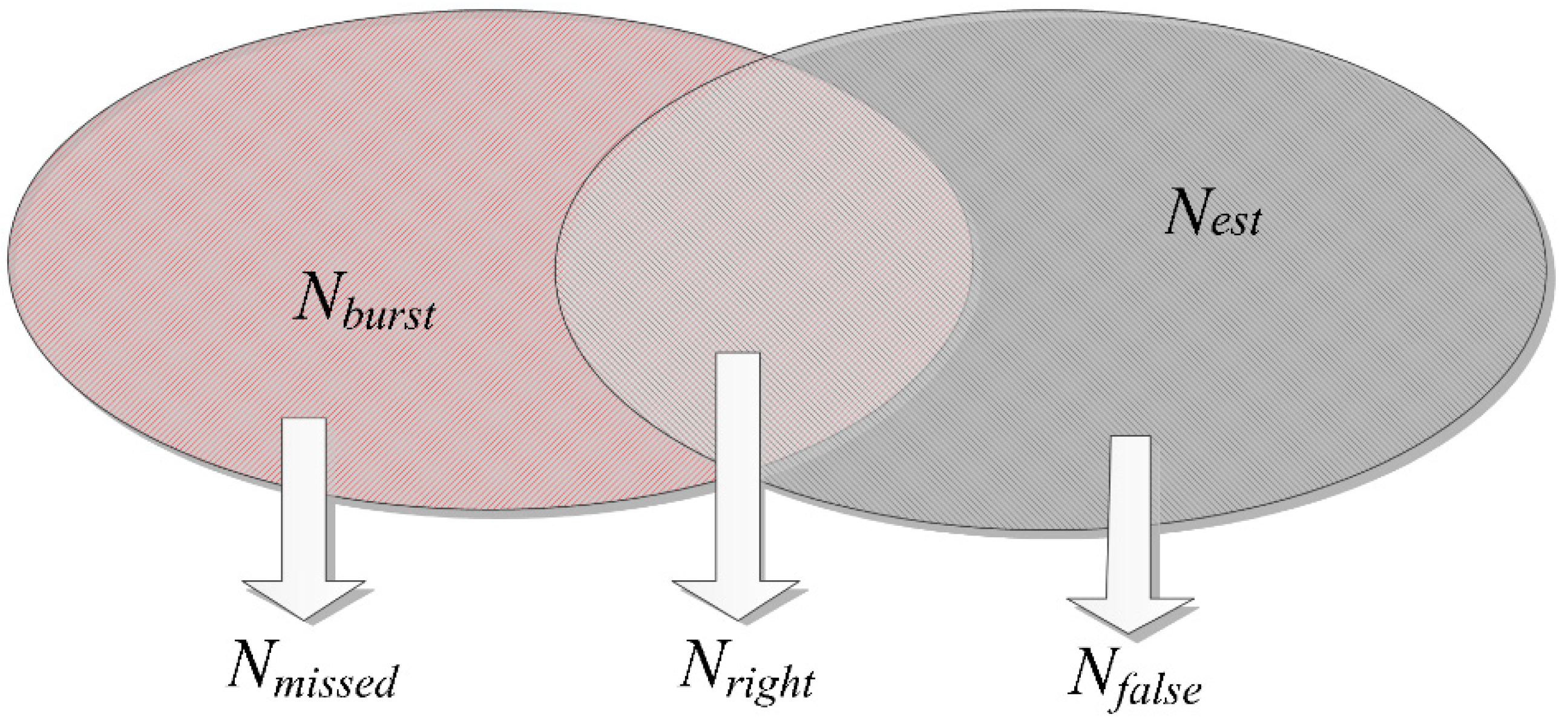
In the regular operation of water distribution system, the ΔPi,t and ΔPs,i,t of a sensor may occasionally surpass the threshold, but this may not necessarily indicate a burst. Other events may induce similar abnormal pressure variations. If enough sensors exceed the thresholds at the same time, there is a high probability that a burst event has occurred. For example, in the case above, nine sensors detected the abnormal event. The minimum number of sensors required to detect an abnormal event is denoted by NS. If the number of sensors that detect abnormal events ≥NS, the monitoring system will initiate an alarm. Thus, the value of NS will influence the accuracy of burst detection. If the value is too low, the monitoring system will initiate many false alarms. If the value is too high, some genuine burst events may be missed. Three detection categories can be used when assessing the capability of a burst event monitoring system [18]: Correct detection, false detection, and missed detection. Nest and Nburst represent the numbers of predicted (i.e., detected by the monitoring system) and observed pipe burst events. Nright is the number of burst events that are both predicted by the system and observed (i.e., correct predictions), Nmissed is the number of burst events that are not predicted but observed, and Nfalse is the number of false alarms (i.e., burst events that are predicted but not observed) The relationships between Nest, Nburst, Nfalse, Nright, and Nmissed are shown in Figure 11.
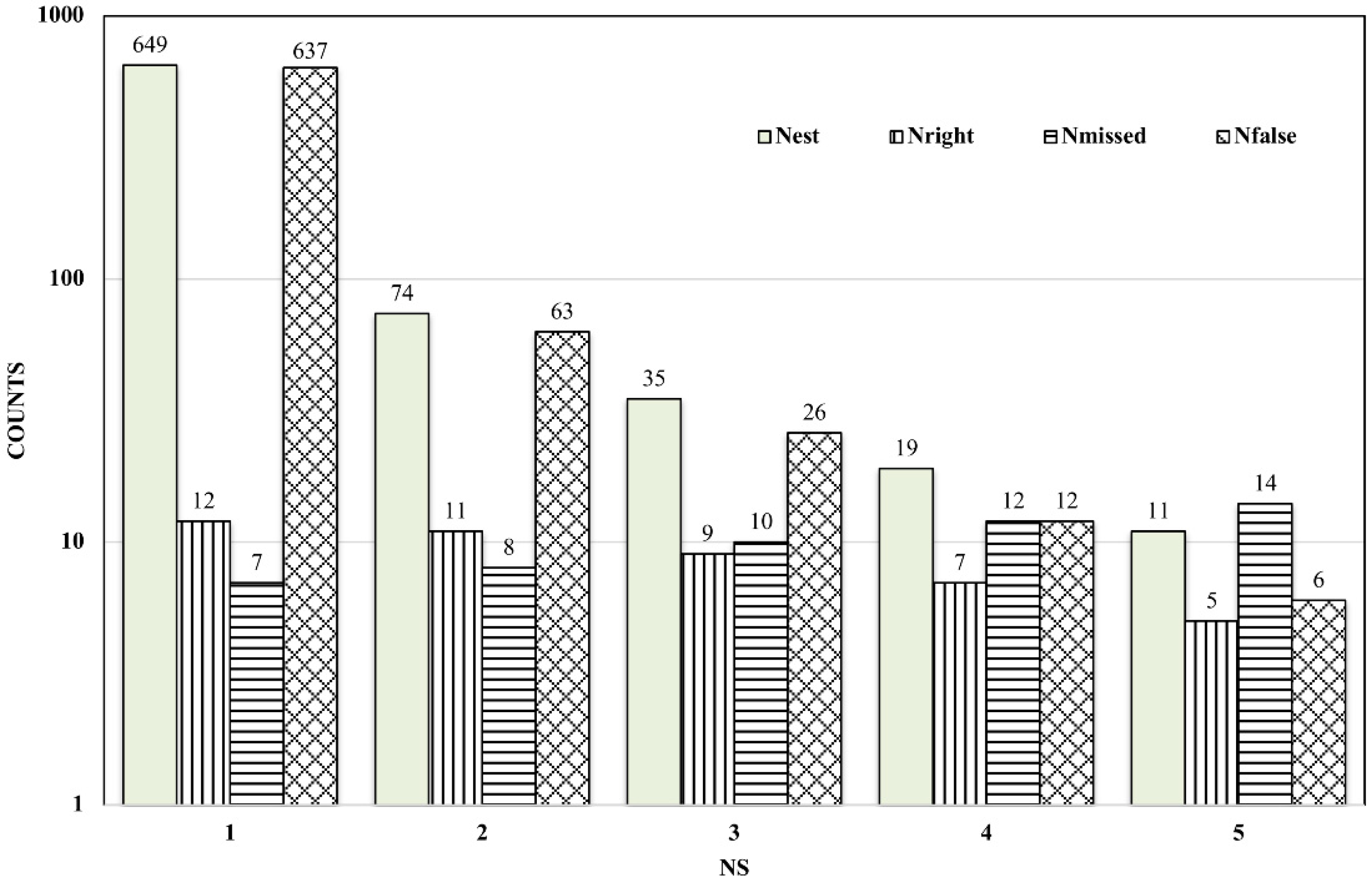
Records of burst events in Guangzhou for one year were used to determine the recommended sensor numbers for burst detection. Nineteen burst events (pipe diameter ≥600 mm) were found, giving Nburst = 19. When the number of sensors exceeding the threshold value is ≥NS, the detection system will create an alarm. The minimum number of sensors to ensure a low false alarm rate can be determined by comparing the results of using different values of NS (Figure 12). When NS = 1, Nfalse is very high. When NS is 2, Nest and Nfalse greatly decrease. When NS > 4, Nmissed will increase rapidly, which means there is a high risk of missing real bursts. These results indicate that for this method to accurately determine burst events, the recommended value of NS is 2 or 3.
6. Conclusions
This paper introduces some basic principles and requirements for the design of a burst event detection system. The thresholds for burst detection and the minimum pipe diameter for which a burst event is detectable were determined. A simple burst detection method was suggested as a result of the statistical analysis of monitoring data and evaluation of the impact of burst events on the WDS. The method was validated using historical records, showing that this method can quickly identify the burst event and give a reasonably accurate burst location. The minimum number of sensors necessary for accurate burst detection was determined for the Guangzhou WDS. The main conclusions and recommendations are as follows:
- (1)
- Monitoring data contain background noise from WDS consumption use and from monitoring equipment. The effect of a detectable burst event should be greater than the level of background noise for a burst event to be correctly identified. The background noise of a pipe system can be determined by statistical analysis of the monitored data using the 3-sigma rule.
- (2)
- The minimum pipe diameter for which a burst event is detectable can be determined by model simulation. Monitoring burst events in pipes of greater than the minimum diameter will improve the burst detection and reduce monitoring costs.
- (3)
- In a detection zone (i.e., the part of the network close to and containing the burst event), a minimum number of sensors is necessary for an acceptable rate of correctly detected burst events. We found that data from two or more sensors close to the burst event location are required to reduce errors due to undetected events and false alarms.
The methods described in this paper for determination of burst thresholds, minimum pipe diameters, burst detection and localization, and minimum sensor numbers were validated using the data for one year from Guangzhou, but they can be used in other applications. The discussion of burst detection algorithms is not within the scope of this paper, so we did not compare the algorithm we used with other methods. However, we think that incorporating evidence theory and Kalman filters would make the prediction of burst events more accurate and thus improve the effectiveness of the SCADA infrastructure.
Author Contributions
Conceptualization, W.C. and G.X.; methodology, W.C.; software, W.C.; validation, G.X., H.F. and D.Z.; formal analysis, W.C.; investigation, G.X.; resources, G.X.; data curation, W.C.; writing—original draft preparation, W.C.; writing—review and editing, W.C. and H.F. supervision, W.C.; project administration, G.X.; funding acquisition, W.C.
Funding
This research received National Nature Science Foundation of China (NSFC Project No. 51578486), the Guangzhou Science and Technology Program (No. 201604020019).
Conflicts of Interest
The authors declare no conflict of interest.
References
- Li, R.; Huang, H.; Xin, K.; Tao, T. A review of methods for burst/leakage detection and location in water distribution systems. Water Sci. Technol. Water Suppl. 2014, 15, 429–441. [Google Scholar] [CrossRef]
- Pudar, R.S.; Liggett, J.A. Leaks in pipe networks. J. Hydraul. Eng. 1992, 118, 1031–1046. [Google Scholar] [CrossRef]
- Vítkovský, J.P.; Simpson, A.R.; Lambert, M.F. Minimization algorithms and experimental inverse transient leak detection. In Proceedings of the 2002 Water Resources Planning and Management Conference, Roanoke, VA, USA, 1 January 2002. [Google Scholar]
- Misiunas, D.; Vitkovsky, J.; Olsson, G.; Simpson, A.R.; Lambert, M.F. Pipeline Burst Detection and Location Using a Continuous Monitoring Technique; Lund University: Lund, Sweden, 2003; pp. 89–96. [Google Scholar]
- Kapelan, Z.; Savic, D.; Walters, G. Incorporation of prior information on parameters in inverse transient analysis for leak detection and roughness calibration. Urban Water J. 2004, 1, 129–143. [Google Scholar] [CrossRef]
- Lee, P.J.; Vítkovský, J.P.; Lambert, M.F.; Simpson, A.R.; Liggett, J.A. Leak location using the pattern of the frequency response diagram in pipelines: A numerical study. J. Sound Vib. 2005, 284, 1051–1073. [Google Scholar] [CrossRef]
- Mounce, S.; Machell, J. Burst detection using hydraulic data from water distribution systems with artificial neural networks. Urban Water J. 2006, 3, 21–31. [Google Scholar] [CrossRef]
- Bicik, J.; Kapelan, Z.; Makropoulos, C.; Savic, D.A. Pipe burst diagnostics using evidence theory. J. Hydroinform. 2011, 13, 596–608. [Google Scholar] [CrossRef]
- Cheng, W.; Fang, H.; Xu, G.; Chen, M. Using SCADA to Detect and Locate Bursts in a Long-Distance Water Pipeline. Water 2018, 10, 1727. [Google Scholar] [CrossRef]
- Ye, G.; Fenner, R.A. Kalman Filtering of Hydraulic Measurements for Burst Detection in Water Distribution Systems. J. Pipeline Syst. Eng. Pract. 2011, 2, 14–22. [Google Scholar] [CrossRef]
- Jung, D.; Lansey, K. Water distribution system burst detection using a nonlinear Kalman filter. J. Water Resour. Plan. Manag. 2014, 141, 04014070. [Google Scholar] [CrossRef]
- Palau, C.V.; Arregui, F.J.; Carlos, M. Burst Detection in Water Networks Using Principal Component Analysis. J. Water Resour. Plan. Manag. 2012, 138, 47–54. [Google Scholar] [CrossRef] [Green Version]
- Romano, M.; Kapelan, Z.; Savić, D.A. Automated detection of pipe bursts and other events in water distribution systems. J. Water Resour. Plan. Manag. 2012, 140, 457–467. [Google Scholar] [CrossRef]
- Jung, D.; Kang, D.; Liu, J.; Lansey, K. Improving the rapidity of responses to pipe burst in water distribution systems: A comparison of statistical process control methods. J. Hydroinform. 2015, 17, 307–328. [Google Scholar] [CrossRef]
- Hagos, M.; Jung, D.; Lansey, K.E. Optimal meter placement for pipe burst detection in water distribution systems. J. Hydroinform. 2016, 18, 741–756. [Google Scholar] [CrossRef] [Green Version]
- Jung, D.; Kim, J.H. Using Mechanical Reliability in Multiobjective Optimal Meter Placement for Pipe Burst Detection. J. Water Resour. Plan. Manag. 2018, 144, 04018031. [Google Scholar] [CrossRef]
- Wang, Y. Study of Pipe Hole Leakage Experiment and Numerical Simulation; Zhejiang University: Hangzhou, China, 2015. [Google Scholar]
- Koch, M.W.; Mckenna, S.A. Distributed Sensor Fusion in Water Quality Event Detection. J. Water Resour. Plan. Manag. 2011, 137, 10–19. [Google Scholar] [CrossRef]
Figure 1.
Schematic of pipe burst monitoring system.

Figure 2.
Requirements for a burst event monitoring system.

Figure 3.
Water distribution system (WDS) in Guangzhou: (A) the area supplied by the Shimen water plant and (B) the 14 sensor locations; the black triangles identify the locations of observed burst events.
Figure 3.
Water distribution system (WDS) in Guangzhou: (A) the area supplied by the Shimen water plant and (B) the 14 sensor locations; the black triangles identify the locations of observed burst events.

Figure 4.
Head and head loss during normal operation and for burst events.

Figure 5.
Pressure and head loss fluctuations (solid line shows observed values; dashed line shows the mean value of observed data ±2 standard deviations).
Figure 5.
Pressure and head loss fluctuations (solid line shows observed values; dashed line shows the mean value of observed data ±2 standard deviations).

Figure 6.
Histograms of pressure drop and head loss parameters.

Figure 7.
Cumulative probability distributions of the pressure (blue plus symbols are observed cumulative probability distributions; solid red lines are the theoretical cumulative normal probability distributions).
Figure 7.
Cumulative probability distributions of the pressure (blue plus symbols are observed cumulative probability distributions; solid red lines are the theoretical cumulative normal probability distributions).

Figure 8.
Calculation of ΔPc i,t and ΔPc s,i,t at sensor 2.

Figure 9.
Pressure drop with (A) D = 1200, n = 1/8, and (B) D = 800, n = 1/2 (triangles are sensors; the red circle is the burst location).
Figure 9.
Pressure drop with (A) D = 1200, n = 1/8, and (B) D = 800, n = 1/2 (triangles are sensors; the red circle is the burst location).

Figure 10.
Pressure drop with (A) D = 600, n = 1/2 and (B) D = 400, n = 1/2 (triangles are sensors; the red circle is the burst location).
Figure 10.
Pressure drop with (A) D = 600, n = 1/2 and (B) D = 400, n = 1/2 (triangles are sensors; the red circle is the burst location).

Figure 11.
Relationships between Nest, Nfalse, Nright, Nburst, and Nmissed.

Figure 12.
Counts of Nest, Nfalse, Nright, and Nmissed.


Table 1.
Pressure drop of burst pipes.
| D (mm) | n | ||||||||
|---|---|---|---|---|---|---|---|---|---|
| 2 | 1 | 1/2 | 1/4 | 1/8 | 1/16 | 1/32 | |||
| 1200 | C | 14,410 | 7200 | 3600 | 1800 | 900 | 450 | 225 | |
| |ΔP|/m | BEP * | 36.435 | 24.783 | 12.749 | 5.939 | 2.726 | 1.304 | 0.674 | |
| 1 | 30.099 | 20.77 | 11.011 | 5.32 | 2.488 | 1.145 | 0.577 | ||
| 9 | 11.232 | 8.086 | 4.823 | 2.439 | 1.157 | 0.562 | 0.274 | ||
| 10 | 8.795 | 6.518 | 3.807 | 1.984 | 0.982 | 0.496 | 0.251 | ||
| 800 | C | 6400 | 3200 | 1600 | 800 | 400 | 200 | 100 | |
| |ΔP|/m | BEP * | 37.599 | 26.622 | 13.414 | 5.988 | 2.707 | 1.468 | 0.99 | |
| 1 | 12.137 | 9.133 | 5.248 | 3.156 | 1.764 | 1.136 | 0.85 | ||
| 9 | 3.973 | 3.142 | 1.934 | 1.328 | 0.794 | 0.532 | 0.403 | ||
| 10 | 2.822 | 2.27 | 1.455 | 1.048 | 0.656 | 0.458 | 0.355 | ||
| 600 | C | 3600 | 1800 | 900 | 450 | 225 | 112 | ||
| |ΔP|/m | BEP * | 23.27 | 11.018 | 4.405 | 2.369 | 1.355 | 0.946 | ||
| 1 | 8.956 | 5.02 | 2.402 | 1.768 | 1.143 | 0.852 | |||
| 9 | 4.141 | 2.373 | 1.209 | 0.883 | 0.576 | 0.425 | |||
| 10 | 3.039 | 1.832 | 0.959 | 0.733 | 0.495 | 0.374 | |||
| 400 | C | 1600 | 800 | 400 | 200 | 100 | |||
| |ΔP|/m | BEP * | 19.966 | 15.887 | 6.182 | 2.667 | 1.306 | |||
| 1 | 4.725 | 2.899 | 1.468 | 1.253 | 0.903 | ||||
| 9 | 1.261 | 0.845 | 0.468 | 0.525 | 0.401 | ||||
| 10 | 0.877 | 0.601 | 0.339 | 0.438 | 0.346 | ||||
| 300 | C | 1600 | 800 | 400 | 200 | ||||
| |ΔP|/m | BEP * | 21.78 | 9.517 | 3.467 | 1.622 | ||||
| 1 | 1.851 | 1.098 | 0.6 | 0.347 | |||||
| 9 | 0.943 | 0.579 | 0.31 | 0.16 | |||||
| 10 | 0.672 | 0.419 | 0.227 | 0.128 | |||||
Note: BEP * denotes the burst event point at which pipe bursts appear.
Table 2.
Threshold values of ΔPi,t and ΔPs,i,t.
| Sensor | 1# | 2# | 3# | 4# | 5# | 6# | 7# | 8# | 9# | 10# | 11# | 12# | 13# | 14# | Average |
|---|---|---|---|---|---|---|---|---|---|---|---|---|---|---|---|
| ΔPc i,t (m) | −1.15 | −1.8 | −1.1 | −1.4 | −1.0 | −1.2 | −1.3 | −1.9 | −1.2 | −1.2 | −1.1 | −1.0 | −1.0 | −1.0 | −1.24 |
| ΔPc s,i,t (m) | 1.38 | 1.45 | 1.4 | 1.8 | 1.4 | 1.6 | 1.9 | 2.0 | 1.4 | 1.6 | 1.4 | 1.5 | 1.5 | 1.6 | 1.57 |
Table 3.
Pressure drop and increase in head loss.
| Node | 1# | 2# | 3# | 4# | 5# | 6# | 7# | 8# | 9# | 10# | 11# | 12# | 13# | 14# |
|---|---|---|---|---|---|---|---|---|---|---|---|---|---|---|
| Prc′ | 0.04 | 0.02 | 0.001 | 0.05 | 0.01 | – | 0.08 | 0.04 | 0.007 | 0.007 | 0.003 | 0.001 | 0.003 | – |
| Prc | 0.98 | 0.98 | 0.80 | 0.93 | 0.97 | – | 0.93 | 0.97 | 0.985 | 0.98 | 0.98 | 0.98 | 0.97 | – |
| ΔPi,t (m) | −3 | −2.9 | −0.4 | −1.4 | −2.3 | – | −1 | −2.4 | −3.3 | −2.9 | −2.7 | −3.3 | −2.4 | – |
| ΔPs,i,t (m) | 3.2 | 3.1 | 0.6 | 1.6 | 2.5 | – | 1.2 | 2.6 | 3.5 | 3.1 | 2.9 | 3.5 | 2.6 | – |
| mark | 1 | 1 | 0 | 0 | 1 | – | 0 | 1 | 1 | 1 | 1 | 1 | 1 | – |
Note: – shows erroneous or missing sensor data; Prc′ is the cumulative probability of pressure drop (ΔPi,t); and Prc is the cumulative probability of head loss increase (ΔPs,i,t).
© 2019 by the authors. Licensee MDPI, Basel, Switzerland. This article is an open access article distributed under the terms and conditions of the Creative Commons Attribution (CC BY) license (http://creativecommons.org/licenses/by/4.0/).
Share and Cite
MDPI and ACS Style
Cheng, W.; Xu, G.; Fang, H.; Zhao, D. Study on Pipe Burst Detection Frame Based on Water Distribution Model and Monitoring System. Water 2019, 11, 1363. https://doi.org/10.3390/w11071363
AMA Style
Cheng W, Xu G, Fang H, Zhao D. Study on Pipe Burst Detection Frame Based on Water Distribution Model and Monitoring System. Water. 2019; 11(7):1363. https://doi.org/10.3390/w11071363
Chicago/Turabian StyleCheng, Weiping, Gang Xu, Hongji Fang, and Dandan Zhao. 2019. "Study on Pipe Burst Detection Frame Based on Water Distribution Model and Monitoring System" Water 11, no. 7: 1363. https://doi.org/10.3390/w11071363
Note that from the first issue of 2016, this journal uses article numbers instead of page numbers. See further details here.