Flash Flood Forecasting Using Support Vector Regression Model in a Small Mountainous Catchment

School of Hydraulic Engineering, Dalian University of Technology, Dalian 116024, China
*
Author to whom correspondence should be addressed.
Water 2019, 11(7), 1327; https://doi.org/10.3390/w11071327
Submission received: 14 April 2019
/
Revised: 21 June 2019
/
Accepted: 21 June 2019
/
Published: 27 June 2019
(This article belongs to the Section Hydrology)
Abstract
:Flash floods in mountainous catchments are often caused by the rainstorm, which may result in more severe consequences than plain area floods due to less timescale and a fast-flowing front of water and debris. Flash flood forecasting is a huge challenge for hydrologists and managers due to its instantaneity, nonlinearity, and dependency. Among different methods of flood forecasting, data-driven models have become increasingly popular in recent years due to their strong ability to simulate nonlinear hydrological processes. This study proposed a Support Vector Regression (SVR) model, which is a powerful artificial intelligence-based model originated from statistical learning theory, to forecast flash floods at different lead times in a small mountainous catchment. The lagged average rainfall and runoff are identified as model input variables, and the time lags associated with the model input variables are determined by the hydrological concept of the time of response. There are 69 flash flood events collected from 1984 to 2012 in a mountainous catchment in China and then used for the model training and testing. The contribution of the runoff variables to the predictions and the phase lag of model outputs are analyzed. The results show that: (i) the SVR model has satisfactory predictive performances for one to three-hours ahead forecasting; (ii) the lagged runoff variables have a more significant effect on the predictions than the rainfall variables; and (iii) the phase lag (time difference) of prediction results significantly exists in both two- and three-hours-ahead forecasting models, however, the input rainfall information can assist in mitigating the phase lag of peak flow.
1. Introduction
Flooding is one of the most serious and frequent disasters worldwide, which causes life loss and structure damage, including buildings, roads, bridges, etc. [1,2]. Climate and land use change are making the frequency of extreme precipitation and flash flood disasters rise [3,4,5]. The changing conditions (e.g., global warming, climate extremes, population growth, etc.,) also largely exaggerate flood risk, which brings more severe challenges to hydrologic forecasters [6,7]. Reliable flood forecasts play a critical role in flood disaster mitigation. Over the past decades, various hydrological models have been developed and broadly used for flood forecasting [8,9,10,11,12,13,14]. In general, these hydrological models can be divided into three categories, namely lumped (e.g., Xinanjiang model), semi-distributed (e.g., TOPMODEL) and distributed models (e.g., SWAT) [15].
However, hydrological models are rarely used for flood forecasting in mountainous catchments due to the limited accuracy of forecasts. The conventional flood forecasting models applied to mountainous catchments are problematic (e.g., short lead time, low accuracy) on account of the strong non-linearity and high uncertainty of the hydrological process in the mountainous area. In addition, it is difficult to predict the flood hydrograph for the mountainous area where sufficient data on rainfall and streamflow are not available, thus hindering the parameter calibration. However, data-driven methods, such as regression, decision trees, and artificial neural network (ANN), have also been employed in flood forecasting [16,17,18,19]. The development of data-driven models largely benefits from advances in computer science and the availability of observed data [20,21]. The data-driven models map the relationship between the model inputs (e.g., rainfall) and outputs (e.g., runoff) which avoid the physical-based hydrological processes, i.e., infiltration, evaporation, etc. The data-driven models are validated to map rainfall into runoff effectively [20,22,23,24,25,26,27,28,29,30,31,32,33].
Machine learning (ML) techniques belong to data-driven methods and have gathered intensive attention with the rapid development of artificial intelligence (AI) worldwide. Support vector regression (SVR), which belongs to the regression scheme of support vector machine (SVM), is a popular and powerful machine learning technique used for solving the regression and classification problems. Over the past decades, the applications of SVR to runoff, river flow or water level predictions have been developed. Yu et al. [34] employed SVR in real-time river stage forecasting and demonstrated that SVR could successfully predict the river stage one- to six-hours ahead. Wu et al. [35] developed a distributed SVR model for river flow prediction, and the proposed model can largely reduce the computational time during the training stage compared with the original SVR model. Yu et al. [36] combined SVM with the Chaos theory to predict daily runoff. Sivapragasam and Liong [37] used different SVR models to predict daily flows in terms of high, medium and low flows, respectively. Lin et al. [38] compared the simulating performance of SVR, ANN, and Autoregressive Moving Average (ARMA) model for forecasting monthly flow discharge, in which the SVR outperforms the other two models.
Besides SVR, other ML techniques, such as artificial neural networks (ANN), decision trees (DT), and adaptive neuro-fuzzy inference systems (ANFIS) etc. have also been applied to hydrological forecasting [39,40,41,42,43,44]. Compared to other ML techniques, SVR has significant advantages as follows: (i) it has the high capability of generalization and is able to adapt various regression and classification problems, since SVR minimizes both the generalization error (e.g., the ability of fitting unknown data) and empirical risk error (e.g., the quality of fitting the training data) [45]. The objectives are set up to achieve a tradeoff between the approximation quality (i.e., empirical risk error) and the trained model complexity (i.e., the generalization error) [46]; (ii) the regression problem of SVR can be expressed as a convex problem (i.e., linear function), and can be solved using global optimization algorithms. Hence, SVR can obtain a global optimal solution; and (iii) SVR can be trained using a relatively small number of training samples since it does not depend on the dimensions of input space [35]. Therefore, the SVR model is selected for hydrological forecasting in this study.
Most of the fore-mentioned studies with respect to data-driven models are focused on long-term forecasting (i.e., days of the week, months of the year), usually involving a specified lead time. However, these studies have seldom investigated the longer lead-time forecasting in SVR. Only one lead time step forecasting cannot satisfy the purpose of practical applications (e.g., flood warning, water resources planning and management etc.). In our view, the hourly-time-step forecasting is essential to the short duration and rapid change of floods in mountainous area. Furthermore, a longer lead-time (e.g., larger than 2 h) forecast is beneficial and adequate for flood evacuation and prevention. Thus, long lead time forecasting at hourly time step using the SVR model is investigated in this study.
The primary goal of this paper is to investigate the predictive capability of SVR for long lead time flood forecasting within a small mountainous catchment. The time lags associated with input variables are determined using a hydrological method, and a two-step grid search method is employed to find optimal parameters of SVR. The rest of this paper is organized as follows: Section 2 presents the basic information of study area as well as the collected observed data used in this study; Section 3 introduces the methodology of SVR including parameter calibration and evaluation indices; the results and discussion are shown in Section 4, and the conclusions are drawn in Section 5.
2. Study Area and Data Sources
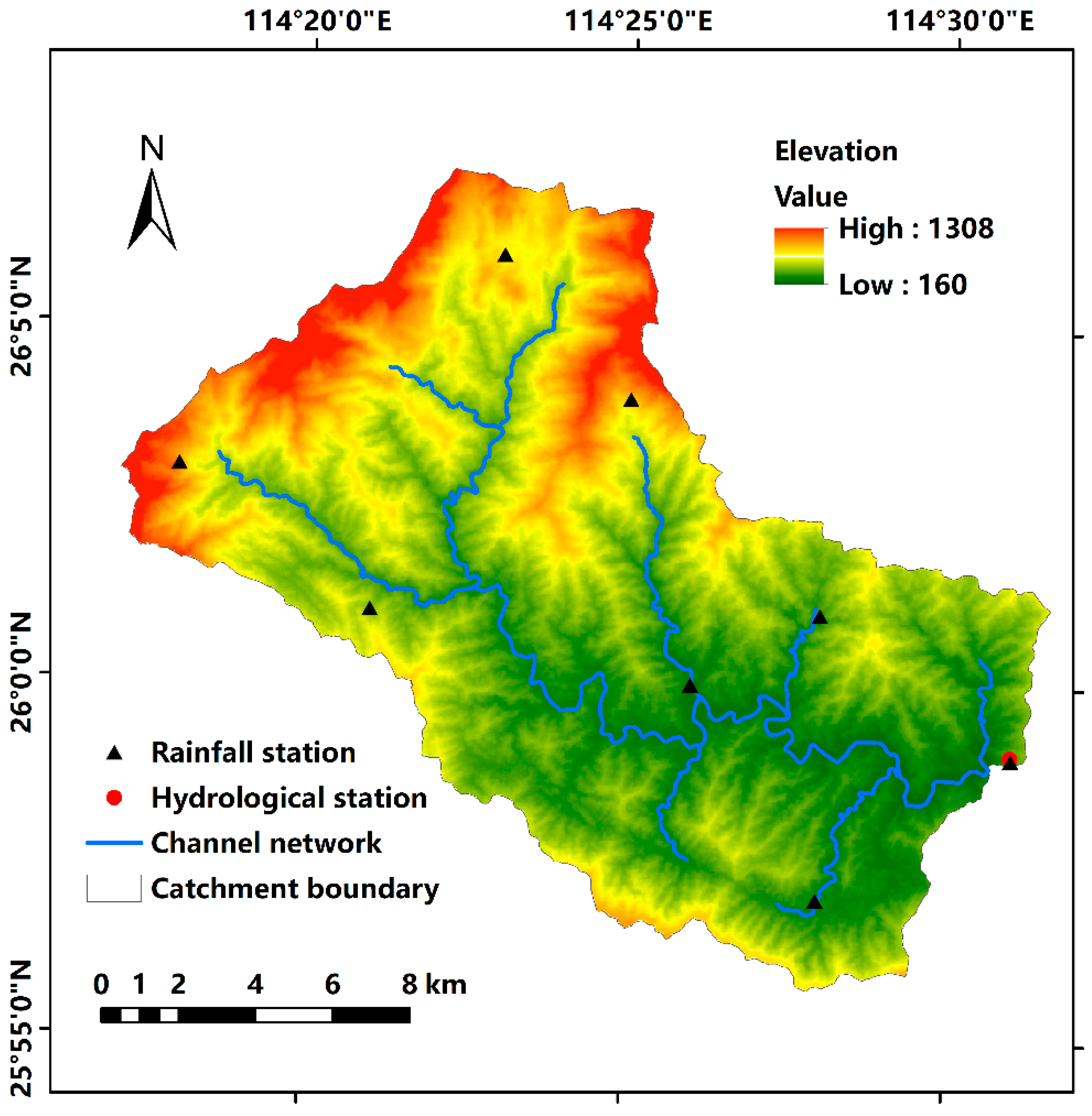
A typical small mountainous catchment Anhe (AH), located in the southwest of the Jiangxi province of China, is used in this study. The AH catchment is shown in Figure 1. The drainage area is 251.0 km2, and the main channel network length is about 79 km. The mean annual precipitation is 1510 mm, and the range of elevation is from 160 m to 1308 m.
The rainfall and discharge data recorded at hourly timestep are collected from the local hydrological bureaus [47] for this study. There are 69 flood events extracted from the data during the period from 1984 to 2012. The 80% data (55 flood events) are used for training, and the remaining 20% (14 flood events) are used for testing. The division of training and testing datasets is based on the chronology. The detailed characteristics of flood events (i.e., rainfall, duration, and peak discharge) are given in supplement material.
The peak flow values range from 71.2 m3/s to 402.5 m3/s in training dataset with the mean value of 143.0 m3/s. The highest peak flow of 561.1 m3/s appears in the testing dataset, which is used to test the extension performance. The average rainfall data is used for this study and calculated based on eight rainfall stations using the Thiessen polygon method, which is reasonable and practical for small catchment where the spatially distributed rainfall information can be neglected. The spatial locations of the rainfall stations are shown in Figure 1.
3. Methodology
3.1. Support Vector Regression
Support vector regression (SVR), which was proposed by Drucker et al. [48], is a model of Support vector machine used for regression. SVR utilizes a hypothesis space of linear function in a high-dimensional feature space and is trained by the structural risk minimization (SRM) principle [34]. The input of SVR is mapped into a high-dimensional feature space using a nonlinear mapping function [35,49]. The detailed description of the SRM principle can be found in the literature [34,35,46,50,51], and the methodology of SVR is introduced in this section [46,48].
In the field of hydrology, most hydrological issues including rainfall-runoff modelling tend to be nonlinear. However, it is extremely difficult to solve nonlinear problems using a linear SVR model due to its limited ability for nonlinearity. The optimal solution is to introduce a nonlinear mapping function to transform input variables into a higher dimensional feature space, in which the original problem may be easily solved using linear regression. Therefore, we applied the nonlinear support vector regression for flood forecasting in this study.
Let represent a set of n samples, where xi and yi are the input vector and corresponding output target values, respectively, and a regression function f(x) can be approximately formulated to depict the nonlinear relationship between the inputs and outputs. The decision function of the SVR model can be written as:
where x is the model input variable vector; w and b are the parameter vectors of the function. ϕ(x) is a nonlinear mapping function. Then, the goal of the SVR algorithm becomes to find the optimal w, b and some internal parameters of ϕ(x). The optimal solution of the SVR algorithm can be obtained by solving the following optimization problem:
where and are slack variables that measure the training errors above and below an tube, and C is a positive constant penalty coefficient that determines the degree of penalized loss when a training error occurs. In Equation (3), the left term represents the generalization of the model, while, the right term reflects the empirical risk, and the objective of SVR is to minimize these two values.
The nonlinear SVR can also be expressed as a dual pattern using the Lagrange Multipliers, and the dual optimization problem of nonlinear SVR can be rewritten as [52,53]:
where ai and ai* are the Lagrange Multipliers; K is the kernel function, which can be calculated by The commonly used kernel functions in SVR include Linear, Radial Basis Function (RBF), Polynomial, and Sigmoid, shown as follows:
1. Linear kernel
2. RBF kernel
3. Polynomial kernel
4. Sigmoid kernel
where γ, d, and r are kernel parameters. γ represents the structural parameters of Polynomial, RBF and Sigmoid kernels. d only exists in Polynomial kernel function and indicates the degree of Polynomial function, and r represents the residuals.
Finally, the decision function of nonlinear SVR can be expressed as:
The SVR model trained is a regression function, and thus the sensitivity analysis of individual input variables can be quantified using the leave-one-out-method (LOOM). To our best knowledge, there is no application of the LOOM in the SVR related studies for sensitivity analysis. The other methods of sensitivity analysis (e.g., Sobol, [54]) can also be used, however, with the consideration of complexity and practicality, the LOOM is used in this study. The LOOM consists of two steps: (1) both runoff and rainfall variables are used as input variables of the trained SVR model, and the predictive results are obtained as a baseline; (2) one of rainfall or runoff inputs is set to be zero. For example, the type of rainfall variables in the input vector are set to zeros, and the predictive results are obtained using only runoff variables. Similarly, the predictive results can also be obtained using only rainfall variables. The predictive results from these three scenarios are drawn in an identical figure for comparison. The detailed sensitivity analysis of different input variables is investigated and presented in Section 4.3 in this paper.
3.2. Input Variables and Normalization
The primary goal of this paper is to build a support regression model to forecast discharge with respect to different lead times at the catchment outlet. For long lead time forecasting, there is a tradeoff between prediction accuracy and forecast lead time. The prediction accuracy declines with the increase in forecast lead time. In our view, the forecast lead time of predictions, at the very least, should be set to three hours, since flood managers can launch flood warnings and inform the people to prepare for possible flooding threat. Meanwhile, we also conducted four- to five-hours-ahead forecasting in this catchment, however, the results are in line with the fore-mentioned accuracy declination trend. Therefore, the longest timestep of outputs is set to three hours according to engineering experience (e.g., time of concentration of runoff in a specific catchment) and practical practice (e.g., trial and error experiments).
For rainfall-runoff modelling, rainfall information is an essential input variable that drives the hydrological processes during the flooding period. Runoff at the outlet is a response to a rainfall event over the catchment. Moreover, the forecasted runoffs are strongly correlated with the historical runoffs. The runoff information has been used as a single model input variable to conduct flood forecasting [55,56,57,58,59], however, it is expected that the additional rainfall information can enhance the predictive performance of data-driven models [31,39,60]. Some studies [61,62,63] adopted additional input variables, e.g., air temperature, evaporation, etc., to conduct stream-flow forecasting, however these effects have trivial impacts on flash floods. Thus, both the lagged rainfall and runoff are selected as the model input variables.
The time lags associated with the input variables should be determined before the SVR model training. We herein utilize the hydrological concept of the time of response to determine the lags of rainfall variables. The differences of appearance time between rainfall and flow peaks are calculated for each flood event. The calculated average of the appearance time difference is 4.84 h and 4.57 h for training and testing datasets, respectively. Therefore, we set the lags of rainfall to 5 h. The lags of runoff are identical to that of rainfall, and the sensitivity analysis on different lags of runoff variable will be presented in the discussion.
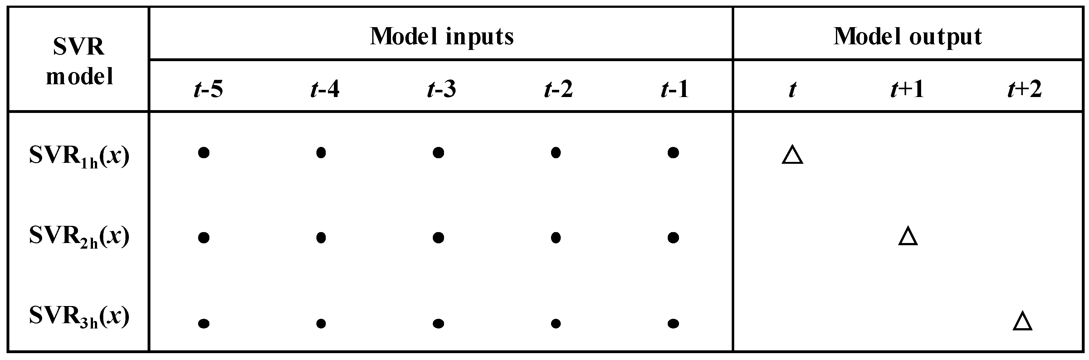
Figure 2 shows the relationship between model inputs and outputs. The black solid points represent the observed lagged rainfall and runoff, while hollow triangles represent the predicted runoff from one to three hours ahead. It should be noted that three SVR models with identical input variables forecast flood runoff from one to three hours ahead, respectively.
Normalization of data is a pre-processing technique and has been widely used for machine learning. For the flood forecasting in this study, the input variables (rainfall and runoff) have different units and their values also largely differ in the order of magnitude. Thus, all input variables are scaled to the range [0, 1] using the MinMaxScaler method, shown as follows:
where X and Xscaled are the unscaled and scaled variable, respectively; Xmax, global and Xmin, global represent the global maximum and minimum value of variables, respectively. In this study, the global statistical values are calculated using all selected flood events, which ensures that all normalized variables are ranged within an identical space.
3.3. Parameter Calibration
The nonlinear SVR model is used for long lead time flood forecasting in this study. A kernel function that maps the input variables into a higher dimensional feature space has to be selected from those commonly used functions (i.e., RBF, Linear, Polynomial, and Sigmoid, etc.). Dibike et al. [50] used different kernel functions in SVR for rainfall-runoff modelling and concluded that the RBF kernel had better performance than other kernel functions. Yang et al. [43] investigated the predictive performances of SVR for reservoir monthly inflow forecasts and demonstrated that SVR using RBF kernel generated more accurate predictions than other kernels. Besides, a large number of previous studies and applications using SVR for hydrological forecasting show that the RBF achieved satisfactory and robust performance [36,51,64]. Therefore, the RBF is selected as the kernel function of SVR in this study.
The performance of SVR highly depends on the hyperparameters including the cost constant C, the radius of the insensitive tube ε, and the kernel parameter γ of RBF function. These parameters are mutually dependent. The cost constant C controls the smoothness of the approximation function (Equation (10)). The greater C value will result in the greater penalty of errors, which the learning model becomes more complex. In contrast, the smaller C value may cause the errors to be excessively tolerated, thus the learning model is poorly approximated. The parameter ε also affects the complexity or smoothness of the approximation function. The value of ε dominates the number of support vectors, which determines the accuracy of the approximation function. The smaller ε value may lead to more support vectors and result in a complex function. The greater ε value may cause the ε-insensitive tube to contain a lot of data that are unseen by the learning model. In this case, some important information may be lost resulting in a poorly flatted approximation function. The kernel parameter γ controls the degree of nonlinearity of the model [65].
The two-step grid search method, the genetic algorithm method, and the shuffled complex evolution algorithm method have been previously used for parameter calibration in SVR [34,35,63,66,67,68]. Hsu [68] recommended the use of two-step grid search method to calibrate parameters due to its significant advantage over time-consuming mitigation. Yu et al. [34] also applied a two-step grid search method to obtain the optimal parameters of different SVR models used for real-time flood stage forecasting. Wu et al. [35] combined the Genetic Algorithm (GA) with the above two-step grid search method to find the optimal parameters and successfully carried out the river flow prediction. In this study, we use the two-step grid search method to determine optimal parameters because of its simplicity, robustness and time-saving. The method consists of two steps. First, a relatively coarser range search (i.e., C = 0.1, 1.0, 10.0, 100.0, 1000.0, 10,000.0, 100,000.0; ε = 0.000001, 0.00001, 0.0001, 0.001, 0.01, 0.1, 1.0; γ = 0.00001, 0.0001, 0.001, 0.01, 0.1, 1.0, 10.0) was applied to obtain the best region of these three-dimensional grids. Then, a smaller range of grid search (e.g., C = 1.0, 10.0, 100.0, 1000.0; ε = 0.0001, 0.001, 0.01; γ = 0.001, 0.01, 0.1) was further conducted to achieve the optimal parameters.
The parameter calibration was completed during the training stage using the training dataset, and then the trained model was evaluated by comparing the testing results using root mean square error (RMSE). The calibrated parameters that achieve good predictive performances in both training and testing datasets are used so that the calibrated model is not trapped in an overfitting problem during the learning stage. The final calibrated parameters for different multiple-hours-ahead SVR models are shown in Table 1.
3.4. Evaluation Indices
For flash floods in a small mountainous catchment, peak flow and time-to-peak (i.e., the appearance time of a peak) are primarily concerned by hydrologists and practitioners, rather than the whole flood hydrograph. In general, the peak flow determines the level of flood risk and can effectively indicate the damage assessment. Meanwhile, peak flow and time-to-peak at the specified cross-section of the river are the vital indicators for flash flood forecasting and warning [69,70,71]. Therefore, the predictions of peak flow and time-to-peak for each flood event in the testing dataset are investigated in this study. Several traditional indices of forecast performance such as the correlation coefficient (R2), the root mean square error (RMSE), the mean absolute error (MAE), the Nash-Sutcliffe efficiency coefficient (NSE), and the relative error (RE), etc., have been widely used for flood forecasting model evaluation in the literature [15,63,72,73,74,75,76]. In this study, the qualified rate (QR) of the number of ‘qualified’ events to the total number of events is calculated based on a national criterion regarding flood forecasting, Standard for Hydrological Information and Hydrological Forecasting [77]. The ‘qualified’ prediction of flood events should satisfy the following indices [77]:
(a) Peak flow:
(b) Time to peak:
where Qm,sim and Qm,obs represent the simulated and observed peak flows, respectively; Tm,obs and Tm,sim represent the peak appearance time of observations and simulations, respectively. Moreover, the fore-mentioned RMSE is averaged among the whole testing flood events for the comprehensive evaluation of all testing flood events.
where N represents the total number of testing flood events; Qij, sim and Qij, obs are the forecasted and observed flows of the ith testing flood event, and ni indicates the length of the ith testing flood event.
The major academic terminologies used in this paper are shown and described in Table 2.
4. Results and Discussion
4.1. Prediction Results
The trained SVR models were used to forecast flood hydrographs with one-, two-, three-hours ahead. The predictive performance of different multiple-hours-ahead models is investigated with respect to the predictions of peak flow and peak appearance time. To avoid the risk of overfitting of SVR models, the predictive statistics of SVR models are calculated for both training and testing datasets. The calculated QR and average RMSE values are shown in Table 3.
As shown in Table 3, the forecasting results are satisfactory, and the testing results are slightly better than the training results as demonstrated by the QR and RMSE values. The three-hours-ahead predictions are worse than that from one- and two-hours-ahead forecasting models. The longer the length of the forecasting period is, the worse predictions obtained.
Figure 3 presents the forecasted and observed peak flows for both the training and testing flood events. The gray shadow represents the uncertainty band of peak flows, and the upper and lower bounds are determined by increasing and decreasing the observed peak flows by 20%, respectively. Most forecasted peak flow values derived from these three SVR models lie in this band. The figure indicates that the forecasted peak flows fit well with the observed peak flows across all flood events. The results from one-hour-ahead SVR model are relatively closer to the observations than that from the other two multiple-hours-ahead SVR models. The highest peak flow during the testing stage was overestimated by all the multiple-hours-ahead models, however, they are still located within the uncertainty band. It is probably because a high variation exists when using SVR to forecast the highest peak flow, which is beyond the peak flow ranges during the training stage. In order to quantify different forecast time horizons of the developed SVR model, the correlation between the observed and predicted peak flows is also shown in Figure 3b,d,f. These figures indicate a relatively good agreement between the observed and predicted peak flows in the selected study area. The dashed black line represents the linear fit, which indicates a strong linear correlation with R2 larger than 0.90.
4.2. Analysis of Runoff Input Variable
The time lags of both rainfall and runoff input variables were set to five hours. The time lags of rainfall variable were determined using the hydrological concept of the time of response, while the runoff variable was aligned with the rainfall variable. In this case, it is possible that the time lags of runoff variable may take significant effect on the predictions.
The different runoff lags are examined with respect to the performance of SVR models. The rainfall variable lags in the input vector are fixed at the maximum value, i.e., five hours, while the runoff variable lags are set from one to five, respectively. The hyperparameters of SVR models are identical to those as shown in Table 1 for a fair comparison. The average RMSE values for all the testing flood events are calculated, as shown in Table 4.
The statistics from Table 4 show that the calculated QR values are identical when runoff variables lagged with one to five hours are used to forecast runoff at one to two hours ahead. In three-hours-ahead forecasting, the forecasts using one- to two-hours-lagged runoff variables are relatively worse when compared to those with more time lags (over two-hours-lagged runoff input variables). Moreover, the differences are less significant among the calculated RMSE values using different lagged runoff variables. That said, more lagged runoff variables can slightly improve the prediction performance of SVR.
4.3. Phase Lag Analysis of Model Output
Phase lag herein refers to the peak appearance time error between the observed and forecasted hydrographs. Table 5 shows the calculated peak appearance time errors for all selected testing flood events. Note that the error values are obtained by subtracting the predicted value from the observed peak appearance time. Most of the error values of the peak appearance time are below zero, which indicates the significant phase lag of predictions. The phase lag will aggravate when using two- and three-hours-ahead SVR models.
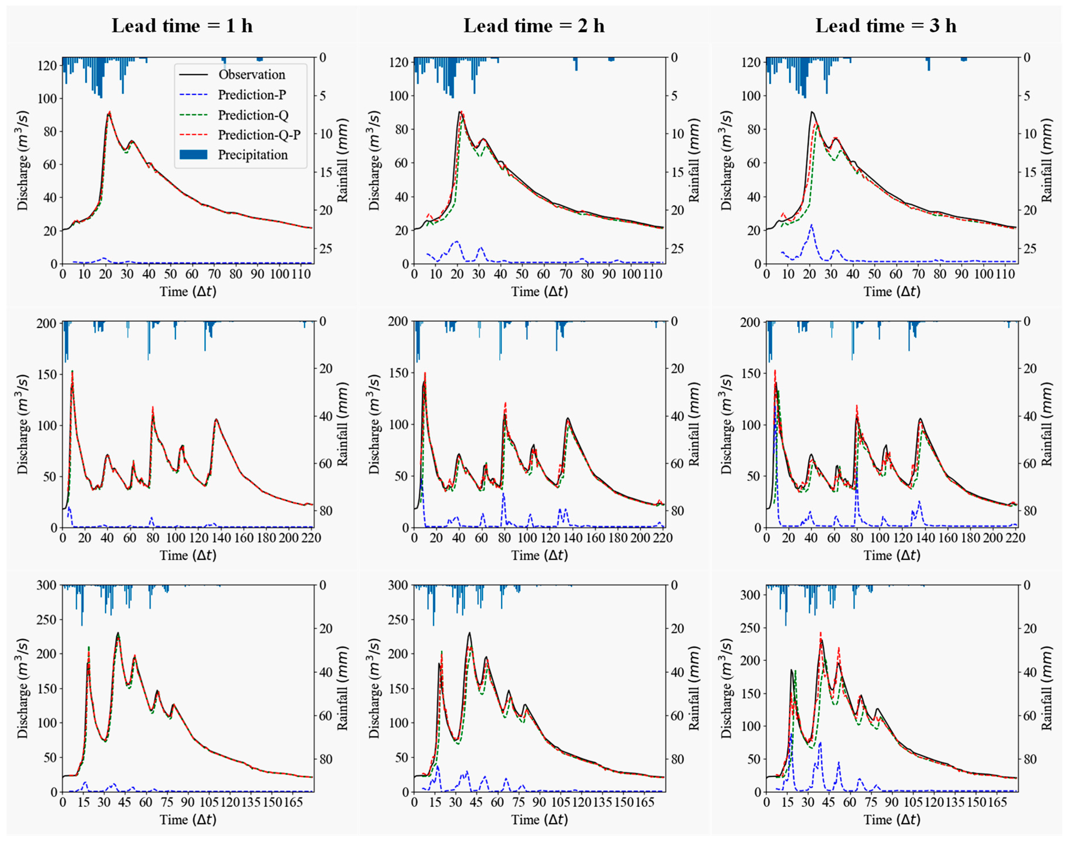
The sensitivity analysis of the model input variables (i.e., rainfall and runoff variables) is investigated with the performance of SVR using LOOM. The predictive results from testing flood events are used for analysis. We selected three typical flood events to describe the impact of rainfall and runoff on the predictions. The typical flood events selected are based on single/multiple peaks, different peak magnitudes. The observed and predicted hydrographs are shown in Figure 4.
As shown in Figure 4, in general, the hydrographs forecasted for longer lead times (e.g., 3 h) present higher deviations and longer phase lags. The hydrographs predicted by the lagged runoff variables are almost in line with the results of both lagged rainfall and runoff variables, which indicate that the lagged runoff variables contribute to the predictions more. In this case, the predicted hydrographs would not decline during the peak stage. The phase lag exists, especially for a longer time ahead forecasting. The input rainfall variables have a significant increasing effect on the high peak flows with the increase in lead time, and the peak appearance time predicted using only lagged rainfall variables are more accurate. Thus, for multiple-hours-ahead (lead time ≥ 2 h) SVR models, it is concluded that the predicted runoff values are dominated by the lagged runoff variables (peak flow magnitude dimension), however, the rainfall variables can largely mitigate the phase lag of model outputs (peak time dimension).
4.4. Discussion on the Potential Application to Larger Regions
In this study, a small mountainous catchment is used to validate the capability of the SVR model of flash flood forecasting at different lead times. As stated previously, the small catchment has the significant characteristics of strong non-linearity and high uncertainty of hydrological processes, which bring difficulties to flood forecasting. The results in this study have shown the advantages of the SVR method. Our study shows that the SVR model presents strong practicality in solving hydrological time series forecasting problems.
Hydrologic and hydraulic models have been widely used to solve flood forecasting problems over large scales [78]. As for data-driven models, the predictive method used in this paper is able to be applied to the large catchment for flood forecasting. In large- or medium-scale catchments, the long forecast horizon of flood forecasting has been investigated, since the flow concentration time will take longer compared with small catchments. Guo et al. [79] utilized an adaptive SVR model to predict monthly streamflow on the Three Gorges Area in the Yangtze River Basin in China. Wang et al. [80] investigated the performance of SVR for forecasting monthly discharge time series in Lancangjiang catchment located in the southwest of China. Huang et al. [81] used a modified Empirical Mode Decomposition based (EMD-based) SVM for monthly streamflow prediction in Wei River basin. In these studies of large catchments, the SVR model shows a good performance on streamflow forecasting.
SVR uses a hypothetical space of linear functions in a highly dimensional feature space in order to achieve a good generalization capability when directly establishing a function between inputs and outputs. As an alternative method, the SVR model shows promising potential applications in the field of hydrology, especially in solving non-linear hydrological problems.
5. Conclusions
This paper proposed a flood forecasting method applied in mountainous areas. The SVR model is utilized to forecast discharge at the river reach from one to three hours ahead. The numerical experiment is carried out using 69 flood events collected in a typical mountainous catchment in China during 29 years. A two-step grid search method is used to determine the hyperparameters of different multiple-hours-ahead SVR models. The time lags of input variables are investigated based on the hydrological concept of the time of response. The peak flow and peak appearance time are used to analyze the predictive performance of SVR.
The SVR models have satisfactory performances to predict the peak flows from one to three hours ahead. The runoff input variable analysis indicates that there is a slight improvement in the prediction results with the increase of input length. The flood forecasts are dominated by the lagged runoff variable, while the rainfall variable has a significant effect on the peak appearance time, especially for the longer time ahead of forecasting. This study shows a strong capability of SVR for long lead time flood forecasting in a mountainous area.
There are several limitations in this study. First, only a small mountainous catchment was selected as the case study since we have collected the abundant rainfall and discharge data, however, future studies are suggested to investigate and compare the predictive performance of SVR in catchments with different spatial scales, topography, and climate conditions (e.g., arid, semi-arid and semi-humid, etc.); Second, the hydrological data during the period from 1984 to 2012 was used in this study, however, the changing conditions (climate and land use changes) in recent years have been enhanced worldwide, and their effects on predictive results are valuable to explore. Meanwhile, other issues, such as the use of different kernel functions, and the comparison of different ML techniques were not presented in this study. More works and efforts should be done to explore these issues in the future.
Author Contributions
J.W. constructed the idea and wrote the manuscript; H.L. revised the manuscript; G.W. and T.S. assisted with the results and discussion section; C.Z. and H.Z. provided feedback on the structure of the manuscript and reviewed the manuscript.
Funding
This research was funded by the National Key Research and Development Program (2017YFC0406001) and the National Natural Science Foundation of China (51708086, 91647201, 91747102).
Acknowledgments
The authors would like to thank the anonymous reviewers and the Associated Editor for their suggestions and comments.
Conflicts of Interest
The authors declare no conflict of interest.
References
- Peduzzi, P. 2009 Global Assessment Report on Disaster Risk Reduction: Patterns, Trends, and Drivers; The UN Office for Disaster Risk Reduction: Geneva, Switzerland, 2009. [Google Scholar]
- Tahir, W.; Jani, J.; Endut, I.R.; Mukri, M.; Kordi, N.E.; Ali, N.E.M. Flood Disaster Management in Malaysia: Standard Operating Procedures (SOPs) Review. In Identification of Seasonal Rainfall Peaks at Kelantan Using Fourier Series; Springer: Berlin/Heidelberg, Germany, 2016. [Google Scholar]
- Kvočka, D.; Falconer, R.; Bray, M. Flood Hazard Assessment for Extreme Flood Events; Springer: Berlin/Heidelberg, Germany, 2016; Volume 84. [Google Scholar]
- Rajib, A.; Merwade, V. Hydrologic response to future land use change in the Upper Mississippi River Basin by the end of 21st century. Hydrol. Process. 2017, 31. [Google Scholar] [CrossRef]
- Du, L.; Rajib, A.; Merwade, V. Large scale spatially explicit modeling of blue and green water dynamics in a temperate mid-latitude basin. J. Hydrol. 2018, 562, 84–102. [Google Scholar] [CrossRef]
- Barros, V.; Stocker, T.F. Managing the risks of extreme events and disasters to advance climate change adaptation: Special report of the Intergovernmental Panel on Climate Change. J. Clin. Endocrinol. Metab. 2012, 18, 586–599. [Google Scholar]
- Hirabayashi, Y.; Mahendran, R.; Koirala, S.; Konoshima, L.; Dai, Y.; Watanabe, S.; Kim, H.; Kanae, S. Global flood risk under climate change. Nat. Clim. Chang. 2013, 3, 816–821. [Google Scholar] [CrossRef]
- Crawford, N.H. Digital Simulation in Hydrology: Stanford Watershed Model IV; Stanford University Technical Reports; Department of Civil Engineering, Stanford University: Stanford, CA, USA, 1966; Volume 39. [Google Scholar]
- Sugawara, M.; Ozaki, E.; Watanabe, I.; Katsuyama, Y. Tank Model and Its Application to Bird Creek, Wollombi Brook, Bikin River, Kitsu River, Sanaga River and Nam Mune; National Research Center for Disaster Prevention: Tokyo, Japan, 1974.
- Zhao, R.J. The Xinanjiang model applied in China. J. Hydrol. 1992, 135, 371–381. [Google Scholar]
- Xu, L. Two-Layer Variable Infiltration Capacity Land Surface Representation for General Circulation Models. Ph.D. Thesis, Washington University, Seattle, WA, USA, 1994. [Google Scholar]
- Bergström, S.; Singh, V.P. The HBV model. In Computer Models of Watershed Hydrology; Singh, V.P., Ed.; Water Resources Publications: Highlands Ranch, CO, USA, 1995; pp. 443–476. [Google Scholar]
- Charley, W.; Pabst, A.; Peters, J. The Hydrologic Modeling System (HEC-HMS): Design and Development Issues. Am. Soc. Civ. Eng. 1995, 1, 131–138. [Google Scholar]
- Zhao, R.J.; Liu, X.R.; Singh, V.P. The Xinanjiang model. Comput. Models Watershed Hydrol. 1995, 135, 371–381. [Google Scholar]
- Wei, G.; Tych, W.; Beven, K.; He, B.; Ning, F.; Zhou, H. Nierji reservoir flood forecasting based on a Data-Based Mechanistic methodology. J. Hydrol. 2018, 567, 227–237. [Google Scholar] [CrossRef]
- Zhu, M.L.; Fujita, M. A Comparison of Fuzzy Inference Method and Neural Network Method for Runoff Prediction. Proc. Hydraul. Eng. 1993, 37, 75–80. [Google Scholar] [CrossRef]
- Zhu, M.L.; Fujita, M.; Hashimoto, N. Application of Neural Networks to Runoff Prediction; Springer: Berlin/Heidelberg, Germany, 1994; pp. 205–216. [Google Scholar]
- Solomatine, D.; See, L.M.; Abrahart, R.J. Data-Driven Modelling: Concepts, Approaches and Experiences; Springer: Berlin/Heidelberg, Germany, 2009; pp. 17–30. [Google Scholar]
- Salas, J.D.; Markus, M.; Tokar, A.S. Streamflow Forecasting Based on Artificial Neural Networks; Springer: Berlin/Heidelberg, Germany, 2000; pp. 23–51. [Google Scholar]
- Kratzert, F.; Klotz, D.; Brenner, C.; Schulz, K.; Herrnegger, M. Rainfall–runoff modelling using Long Short-Term Memory (LSTM) networks. Hydrol. Earth Syst. Sci. 2018, 22, 6005–6022. [Google Scholar] [CrossRef]
- Schmidhuber, J. Deep learning in neural networks: An overview. Neural Netw. 2015, 61, 85–117. [Google Scholar] [CrossRef] [PubMed] [Green Version]
- Sajikumar, N.; Thandaveswara, B.S. A non-linear rainfall–runoff model using an artificial neural network. J. Hydrol. 1999, 216, 32–55. [Google Scholar] [CrossRef]
- Tokar, A.S.; Johnson, P.A. Rainfall-Runoff Modeling Using Artificial Neural Networks. J. Hydrol. Eng. 1999, 4, 232–239. [Google Scholar] [CrossRef]
- Sivapragasam, C.; Liong, S.-Y.; Pasha, F. Rainfall and runoff forecasting with SSA-SVM approach. J. Hydroinform. 2001, 3, 213–217. [Google Scholar] [CrossRef]
- Pan, T.Y.; Wang, R.Y. Using recurrent neural networks to reconstruct rainfall-runoff processes. Hydrol. Process. 2010, 19, 3603–3619. [Google Scholar] [CrossRef]
- Guo, R.; Zhao, F.; Yanan, L.I. Dynamic modeling of rainfall-runoff process in river basin with recurrent wavelet neural network. J. Hydroelectr. Eng. 2013, 32, 54–59. [Google Scholar]
- Hosseini, S.M.; Mahjouri, N. Integrating Support Vector Regression and a geomorphologic Artificial Neural Network for daily rainfall-runoff modeling. Appl. Soft Comput. 2016, 38, 329–345. [Google Scholar] [CrossRef]
- Wang, W.-C.; Chau, K.-W.; Qiu, L.; Chen, Y.-B. Improving forecasting accuracy of medium and long-term runoff using artificial neural network based on EEMD decomposition. Environ. Res. 2015, 139, 46–54. [Google Scholar] [CrossRef]
- Ali Ghorbani, M.; Kazempour, R.; Chau, K.-W.; Shamshirband, S.; Taherei Ghazvinei, P. Forecasting pan evaporation with an integrated artificial neural network quantum-behaved particle swarm optimization model: A case study in Talesh, Northern Iran. Eng. Appl. Comput. Fluid Mech. 2018, 12, 724–737. [Google Scholar] [CrossRef]
- Moazenzadeh, R.; Mohammadi, B.; Shamshirband, S.; Chau, K.-W. Coupling a firefly algorithm with support vector regression to predict evaporation in northern Iran. Eng. Appl. Comput. Fluid Mech. 2018, 12, 584–597. [Google Scholar] [CrossRef] [Green Version]
- Wu, C.L.; Chau, K.W. Rainfall–runoff modeling using artificial neural network coupled with singular spectrum analysis. J. Hydrol. 2011, 399, 394–409. [Google Scholar] [CrossRef]
- Chuntian, C.; Chau, K.W. Three-person multi-objective conflict decision in reservoir flood control. Eur. J. Oper. Res. 2002, 142, 625–631. [Google Scholar] [CrossRef] [Green Version]
- Yaseen, Z.M.; Sulaiman, S.O.; Deo, R.C.; Chau, K.-W. An enhanced extreme learning machine model for river flow forecasting: State-of-the-art, practical applications in water resource engineering area and future research direction. J. Hydrol. 2019, 569, 387–408. [Google Scholar] [CrossRef]
- Yu, P.-S.; Chen, S.-T.; Chang, I.F. Support Vector Regression for Real-Time Flood Stage Forecasting. J. Hydrol. 2006, 328, 704–716. [Google Scholar] [CrossRef]
- Wu, C.L.; Chau, K.W.; Li, Y.S. River stage prediction based on a distributed support vector regression. J. Hydrol. 2008, 358, 96–111. [Google Scholar] [CrossRef] [Green Version]
- Yu, X.; Liong, S.Y.; Babovic, V. EC-SVM approach for real-time hydrologic forecasting. J. Hydroinform. 2004, 6, 209–223. [Google Scholar] [CrossRef] [Green Version]
- Sivapragasam, C.; Liong, S.-Y. Flow categorization model for improving forecasting. Hydrol. Res. 2005, 36, 37–48. [Google Scholar] [CrossRef]
- Lin, J.Y.; Cheng, C.T.; Chau, K.W. Using support vector machines for long-term discharge prediction. Hydrol. Sci. J. 2006, 51, 599–612. [Google Scholar] [CrossRef]
- Badrzadeh, H.; Sarukkalige, R.; Jayawardena, A.W. Hourly runoff forecasting for flood risk management: Application of various computational intelligence models. J. Hydrol. 2015, 529, 1633–1643. [Google Scholar] [CrossRef]
- Kumar, A.R.S.; Singh, R.D.; Swamee, P.K.; Nema, R.K. Application of ANN, Fuzzy Logic and Decision Tree Algorithms for the Development of Reservoir Operating Rules. Water Resour. Manag. 2013, 27, 911–925. [Google Scholar] [CrossRef]
- Yang, T.; Gao, X.; Sorooshian, S.; Li, X. Simulating California reservoir operation using the classification and regression-tree algorithm combined with a shuffled cross-validation scheme. Water Resour. Res. 2016, 52, 1626–1651. [Google Scholar] [CrossRef] [Green Version]
- Naghibi, S.A.; Ahmadi, K.; Daneshi, A. Application of Support Vector Machine, Random Forest, and Genetic Algorithm Optimized Random Forest Models in Groundwater Potential Mapping. Water Resour. Manag. 2017, 31, 2761–2775. [Google Scholar] [CrossRef]
- Yang, T.; Asanjan, A.A.; Welles, E.; Gao, X.; Sorooshian, S.; Liu, X. Developing reservoir monthly inflow forecasts using artificial intelligence and climate phenomenon information. Water Resour. Res. 2017, 53, 2786–2812. [Google Scholar] [CrossRef]
- Liu, Y.; Ye, L.; Qin, H.; Hong, X.; Ye, J.; Yin, X. Monthly streamflow forecasting based on hidden Markov model and Gaussian Mixture Regression. J. Hydrol. 2018, 561, 146–159. [Google Scholar] [CrossRef]
- Kecman, V. Learning and Soft Computing-Support Vector Machines, Neural Networks, Fuzzy Logic Systems; The MIT Press: Cambridge, MA, USA, 2001. [Google Scholar]
- Vapnik, V.N. An overview of statistical learning theory. IEEE Trans. Neural Netw. 1999, 10, 988–999. [Google Scholar] [CrossRef] [PubMed]
- Guo, L.; Zhang, C.; Zhou, H.; Ye, L.; Song, T.; Wu, J. Applicability Analysis of Hydrological Model in Small Mountanious Catchment; China Institute of Water Resources and Hydropower Research: Beijing, China, 2017; (Report In Chinese). [Google Scholar]
- Drucker, H.; Burges, C.J.C.; Kaufman, L.; Smola, A.J.; Vapnik, V.N. Support Vector Regression Machines. In Proceedings of the NIPS on Advances in Neural Information Processing Systems 9, Denver, CO, USA, 3–5 December 1996; pp. 155–161. [Google Scholar]
- Wu, M.C.; Lin, G.F.; Lin, H.-Y. Improving the forecasts of extreme streamflow by support vector regression with the data extracted by self-organizing map. Hydrol. Process. 2014, 28, 386–397. [Google Scholar] [CrossRef]
- Dibike, Y.B.; Velickov, S.; Solomatine, D.; Abbott, M.B. Model Induction With Support Vector Machines: Introduction and Applications. J. Comput. Civ. Eng. 2001, 15, 208–216. [Google Scholar] [CrossRef]
- Liong, S.-Y.; Chandrasekaran, S. Flood Stage Forecasting With Support Vector Machines. J. Am. Water Resour. Assoc. 2007, 38, 173–186. [Google Scholar] [CrossRef]
- Chang, C.C.; Lin, C.J. LIBSVM: A library for support vector machines. ACM Trans. Intern. Syst. Technol. 2001, 2, 1–27. [Google Scholar] [CrossRef]
- Gunn, S.R. Support vector machines for classification and regression. Tech. Rep. Image Speech Intell. Syst. Res. Group 1997, 1, 1–52. [Google Scholar]
- Chi, Z.; Chu, J.; Fu, G. Sobol’s sensitivity analysis for a distributed hydrological model of Yichun River Basin, China. J. Hydrol. 2013, 480, 58–68. [Google Scholar]
- Cigizoglu, H.K. Application of Generalized Regression Neural Networks to Intermittent Flow Forecasting and Estimation. J. Hydrol. Eng. 2005, 10, 336–341. [Google Scholar] [CrossRef]
- Jain, A.; Kumar, A.M. Hybrid neural network models for hydrologic time series forecasting. Appl. Soft Comput. 2007, 7, 585–592. [Google Scholar] [CrossRef]
- Chen, C.-S.; Liu, C.-H.; Su, H.-C. A nonlinear time series analysis using two-stage genetic algorithms for streamflow forecasting. Hydrol. Process. 2008, 22, 3697–3711. [Google Scholar] [CrossRef]
- Carrier, C.; Kalra, A.; Ahmad, S. Using Paleo Reconstructions to Improve Streamflow Forecast Lead Time in the Western United States. J. Am. Water Resour. Assoc. 2013, 49, 1351–1366. [Google Scholar] [CrossRef]
- Danandeh Mehr, A.; Kahya, E.; Olyaie, E. Streamflow prediction using linear genetic programming in comparison with a neuro-wavelet technique. J. Hydrol. 2013, 505, 240–249. [Google Scholar] [CrossRef]
- Li, P.-H.; Kwon, H.-H.; Sun, L.; Lall, U.; Kao, J.-J. A modified support vector machine based prediction model on streamflow at the Shihmen Reservoir, Taiwan. Int. J. Climatol. 2010, 30, 1256–1268. [Google Scholar] [CrossRef]
- Makkeasorn, A.; Chang, N.B.; Zhou, X. Short-term streamflow forecasting with global climate change implications—A comparative study between genetic programming and neural network models. J. Hydrol. 2008, 352, 336–354. [Google Scholar] [CrossRef]
- Behzad, M.; Asghari, K.; Eazi, M.; Palhang, M. Generalization performance of support vector machines and neural networks in runoff modeling. Expert Syst. Appl. 2009, 36, 7624–7629. [Google Scholar] [CrossRef]
- Noori, R.; Karbassi, A.R.; Moghaddamnia, A.; Han, D.; Zokaei-Ashtiani, M.H.; Farokhnia, A.; Gousheh, M.G. Assessment of input variables determination on the SVM model performance using PCA, Gamma test, and forward selection techniques for monthly stream flow prediction. J. Hydrol. 2011, 401, 177–189. [Google Scholar] [CrossRef]
- Bray, M.; Han, D. Identification of support vector machines for runoff modelling. J. Hydroinform. 2004, 6, 265–280. [Google Scholar] [CrossRef] [Green Version]
- Tien Bui, D.; Pradhan, B.; Löfman, O.; Revhaug, I. Landslide Susceptibility Assessment in Vietnam Using Support Vector Machines, Decision Tree, and Naïve Bayes Models. Math. Probl. Eng. 2012, 2012, 26. [Google Scholar] [CrossRef]
- Su, J.; Wang, X.; Liang, Y.; Chen, B. GA-Based Support Vector Machine Model for the Prediction of Monthly Reservoir Storage. J. Hydrol. Eng. 2014, 19, 1430–1437. [Google Scholar] [CrossRef]
- Jiao, B.; Xiang Xu, Z. Nonlinear Inertia Weigh Particle Swarm Optimization Combines Simulated Annealing Algorithm and Application in Function and SVM Optimization. Appl. Mech. Mater. 2011, 130–134, 3467–3471. [Google Scholar] [CrossRef]
- Hsu, C.W. A Practical Guide to Support Vector Classification. 2003. Available online: http://www.csie.ntu.edu.tw/~cjlin/paper/guide.pdf (accessed on 3 April 2019).
- Liu, C.; Guo, L.; Ye, L.; Zhang, S.; Zhao, Y.; Song, T. A review of advances in China’s flash flood early-warning system. Nat. Hazards 2018, 92, 619–634. [Google Scholar] [CrossRef]
- Suntaranont, B.; Aryupong, C.; Jankoo, S.; Champrasert, P. Energy aware flash flood monitoring stations using a GA-fuzzy logic control mechanism. In Proceedings of the IEEE Tenth International Conference on Intelligent Sensors, Sensor Networks and Information Processing (ISSNIP), Singapore, 7–9 April 2015. [Google Scholar]
- Koutroulis, A.G.; Tsanis, I.K. A method for estimating flash flood peak discharge in a poorly gauged basin: Case study for the 13–14 January 1994 flood, Giofiros basin, Crete, Greece. J. Hydrol. 2010, 385, 150–164. [Google Scholar] [CrossRef]
- Asefa, T.; Kemblowski, M.; McKee, M.; Khalil, A. Multi-time scale stream flow predictions: The support vector machines approach. J. Hydrol. 2006, 18, 7–16. [Google Scholar] [CrossRef]
- Danandeh Mehr, A.; Kahya, E.; Şahin, A.; Nazemosadat, M.J. Successive-station monthly streamflow prediction using different artificial neural network algorithms. Int. J. Environ. Sci. Technol. 2015, 12, 2191–2200. [Google Scholar] [CrossRef]
- Nayak, P.C.; Sudheer, K.P.; Jain, S.K. Rainfall-runoff modeling through hybrid intelligent system. Water Resour. Res. 2007, 43. [Google Scholar] [CrossRef]
- Chang, F.-J.; Chen, Y.-C. A counterpropagation fuzzy-neural network modeling approach to real time streamflow prediction. J. Hydrol. 2001, 245, 153–164. [Google Scholar] [CrossRef]
- Wu, J.S.; Han, J.; Annambhotla, S.; Bryant, S. Artificial Neural Networks for Forecasting Watershed Runoff and Stream Flows. J. Hydrol. Eng. 2005, 10, 216–222. [Google Scholar] [CrossRef]
- Ministry of Water Resource. Standard for Hydrological Information and Hydrological Forecasting; China Standards Press: Beijing, China, 2008. (In Chinese)
- Merwade, V.; Rajib, A.; Liu, Z. An Integrated Approach for Flood Inundation Modeling on Large Scales. In Bridging Science and Policy Implication for Managing Climate Extremes; World Scientific Publication Company: Singapore, 2018; pp. 133–155. [Google Scholar]
- Guo, J.; Zhou, J.; Qin, H.; Zou, Q.; Li, Q. Monthly streamflow forecasting based on improved support vector machine model. Expert Syst. Appl. 2011, 38, 13073–13081. [Google Scholar] [CrossRef]
- Wang, W.-C.; Chau, K.-W.; Cheng, C.-T.; Qiu, L. A comparison of performance of several artificial intelligence methods for forecasting monthly discharge time series. J. Hydrol. 2009, 374, 294–306. [Google Scholar] [CrossRef] [Green Version]
- Huang, S.; Chang, J.; Huang, Q.; Chen, Y. Monthly streamflow prediction using modified EMD-based support vector machine. J. Hydrol. 2014, 511, 764–775. [Google Scholar] [CrossRef]
Figure 1.
Map for the Anhe (AH) catchment.

Figure 2.
Relationship between model inputs and outputs.

Figure 3.
Comparison between the predicted and observed peak flows: (a,b) Lead time = 1 h; (c,d) Lead time = 2 h; (e,f) Lead time = 3 h.
Figure 3.
Comparison between the predicted and observed peak flows: (a,b) Lead time = 1 h; (c,d) Lead time = 2 h; (e,f) Lead time = 3 h.

Figure 4.
Forecasting results using different input variables.


Table 1.
Calibrated parameters of different Support Vector Regression (SVR) models.
| Lead Time (h) | Calibrated Parameters | ||
|---|---|---|---|
| C | ε | γ | |
| 1 | 100.0 | 0.0001 | 0.01 |
| 2 | 1000.0 | 0.0001 | 0.001 |
| 3 | 1000.0 | 0.001 | 0.01 |
Table 2.
Notations.
| Name | Definition | Unit |
|---|---|---|
| lagged runoff variable | antecedent runoff variable, for example, given that Q(t) represents the forecasted runoff at t timestep, Q(t − 1), Q(t − 2), and Q(t − 3) etc. are the lagged runoff variables used for predicting runoff at t timestep. | m3/s |
| phase lag | the time error between the observed and forecasted peak flow within individual flood event | h |
| peak appearance time | the time to peak flow | h |
| Prediction-P | the runoff prediction is obtained using only rainfall variables | m3/s |
| Prediction-Q | the runoff prediction is obtained using only runoff variables | m3/s |
| Prediction-Q-P | the runoff prediction is obtained using both runoff and rainfall variables | m3/s |
Table 3.
Statistics of prediction results.
| Lead Time (h) | QR | RMSE (m3/s) | ||
|---|---|---|---|---|
| Training | Testing | Training | Testing | |
| 1 | 0.945 | 1.000 | 12.9 | 4.1 |
| 2 | 0.927 | 1.000 | 28.4 | 10.1 |
| 3 | 0.709 | 0.786 | 32.3 | 12.2 |
Table 4.
Comparisons of predictions using different lags of runoff variable.
| Lead Time (h) | QR | RMSE (m3/s) | |||||||||
|---|---|---|---|---|---|---|---|---|---|---|---|
| 1 h | 2 h | 3 h | 4 h | 5 h | 1 h | 2 h | 3 h | 4 h | 5 h | ||
| 1 | 0.929 | 1.000 | 1.000 | 1.000 | 1.000 | 6.078 | 4.741 | 4.242 | 4.136 | 4.061 | |
| 2 | 0.929 | 1.000 | 1.000 | 1.000 | 1.000 | 11.583 | 10.844 | 10.104 | 10.107 | 10.058 | |
| 3 | 0.714 | 0.714 | 0.786 | 0.786 | 0.786 | 13.495 | 13.602 | 13.049 | 12.457 | 12.241 | |
Table 5.
Calculated peak appearance time errors for all selected testing flood events at different lead times (LT).
Table 5.
Calculated peak appearance time errors for all selected testing flood events at different lead times (LT).
| Flood Event | LT = 1 h | LT = 2 h | LT = 3 h |
|---|---|---|---|
| Event 56 | 0 | −1 | 2 |
| Event 57 | 0 | −1 | −2 |
| Event 58 | 0 | −1 | −2 |
| Event 59 | −1 | −1 | −2 |
| Event 60 | −1 | −1 | 1 |
| Event 61 | −1 | −2 | −2 |
| Event 62 | 0 | −1 | 0 |
| Event 63 | 0 | −1 | 1 |
| Event 64 | −1 | −2 | 1 |
| Event 65 | 0 | −1 | −5 |
| Event 66 | −1 | −2 | −2 |
| Event 67 | −1 | −1 | 1 |
| Event 68 | −1 | −1 | −1 |
| Event 69 | 0 | −1 | 1 |
© 2019 by the authors. Licensee MDPI, Basel, Switzerland. This article is an open access article distributed under the terms and conditions of the Creative Commons Attribution (CC BY) license (http://creativecommons.org/licenses/by/4.0/).
Share and Cite
MDPI and ACS Style
Wu, J.; Liu, H.; Wei, G.; Song, T.; Zhang, C.; Zhou, H. Flash Flood Forecasting Using Support Vector Regression Model in a Small Mountainous Catchment. Water 2019, 11, 1327. https://doi.org/10.3390/w11071327
AMA Style
Wu J, Liu H, Wei G, Song T, Zhang C, Zhou H. Flash Flood Forecasting Using Support Vector Regression Model in a Small Mountainous Catchment. Water. 2019; 11(7):1327. https://doi.org/10.3390/w11071327
Chicago/Turabian StyleWu, Jian, Haixing Liu, Guozhen Wei, Tianyu Song, Chi Zhang, and Huicheng Zhou. 2019. "Flash Flood Forecasting Using Support Vector Regression Model in a Small Mountainous Catchment" Water 11, no. 7: 1327. https://doi.org/10.3390/w11071327
Note that from the first issue of 2016, this journal uses article numbers instead of page numbers. See further details here.