Application of a Parallel Particle Swarm Optimization-Long Short Term Memory Model to Improve Water Quality Data

Abstract

Water quality data cleaning is important for the management of water environments. A framework for water quality time series cleaning is proposed in this paper. Considering the nonlinear relationships among water quality indicators, support vector regression (SVR) is used to forecast water quality indicators when some indicators are missing or when they show abnormal values at a certain point in time. Considering the time series of water quality information, long short-term memory (LSTM) networks are used to forecast water quality indicators when all indicators are missing at a certain point in time. A parallel model based on particle swarm optimization (PSO) and LSTM is realized based on a microservices architecture to improve the efficiency of model execution and the predictive accuracy of the LSTM networks. The performance of the model is evaluated in terms of the mean absolute error (MAE) and root-mean-square error (RMSE). Inlet water quality data from a wastewater treatment plant in Gaobeidian, Beijing, China is considered as a case study to examine the effectiveness of this approach. The experimental results reveal that this model has better predictive accuracy than other data-driven models because of smaller MAE and RMSE and has an advantage in terms of time consumption compared with standalone serial algorithms.

1. Introduction

Accurate and effective forecasting of water quality is important for water environment management and for properly studying aqueous ecological systems. With the development of water quality assessment, increasingly more water quality time series must be effectively analyzed and processed. Water quality data cleaning is an indispensable task before water quality data mining, as it provides a guarantee for people to obtain complete and high-quality datasets. The main task of data cleaning is to find abnormal values and fill in missing values.

Machine learning models have proven to be useful tools because they offer relatively high efficiency and accuracy when dealing with complicated water quality forecasting problems. For example, artificial neural networks (ANNs) and support vector machines (SVMs) are representative machine learning models [1]. In addition, several other machine learning methods have been used, including Bayesian networks [2], logistic regression [3] and wavelet neural networks [4]. Long short-term memory (LSTM) networks, which are a class of recurrent neural networks, are suitable for processing and predicting important events with relatively long intervals and delays in the corresponding time series [5]. These networks have been successfully applied in the field of water time series prediction. For example, Jian Zhou used an LSTM network to predict dissolved oxygen [6] and Chen Liang used an LSTM network to predict the Dongting Lake water level variation [7]. However, the prediction accuracy of the LSTM algorithm used in these studies is influenced by the parameter selection. Therefore, this paper uses a PSO algorithm to optimize the parameter selection in LSTM networks (referred to as a parallel PSO-LSTM model for short). PSO is a computational method of solving an optimization problem by iteratively attempting to improve a candidate solution with regard to a given measure of quality. For example, the results of applying a PSO-based optimal SVR model for the prediction of ammonia nitrogen and a PSO-based optimal ANN model for the early detection of dengue disease suggest that PSO algorithms can accelerate the training of machine learning models and improve the training accuracy [8,9].

With the development of water data collection, the high complexity of computations in machine learning and optimization algorithms leads to high requirements for single-node computing. In this paper, this problem is resolved by using a microservices architecture. A microservices architecture is a type of technology architecture to realize a distributed environment, which is mainly realized by network programming [10]. For example, Michael Schmidt used a microservices architecture to improve the fault tolerance of Ambient Assisted Living (AAL) systems [11] and Marc Dalmau used a microservices architecture to reduce the energy consumption of network devices [12]. In this paper, the microservices architecture is realized by using Java and Python web technology.

Based on multivariate correlations among water quality information and time series characteristics, a framework for water quality data cleaning based on a parallel PSO-LSTM model is proposed in this paper. First, the original data are cleaned by calculating Z-scores. Then, SVR is used to fill in data when some indicators are missing or when they show abnormal values at a certain point in time. Second, LSTM is used to forecast water quality indicators when all indicators are missing at a certain point in time. Finally, using the constructed model, the mean absolute error and the root-mean-square error model execution time are compared and the efficiency and accuracy of the method are evaluated.

The contributions of this paper are as follows: (1) a data cleaning automation process is established for water quality time series; (2) a parallel PSO-LSTM model based on a microservices architecture is proposed to handle complex calculations in less time and increase predictive accuracy.

The remainder of this paper is structured as follows. Section 2 introduces the algorithms and model used in this paper. Section 3 presents the parallel PSO-LSTM model based on the microservices architecture. Experimental results are discussed in Section 4. Finally, the conclusions of this article and future work are discussed in Section 5.

2. Materials and Methods

2.1. SVR

The SVM method was first proposed by Vapnik in 1995. The SVM method is theoretically based on statistical learning theory, namely, an approximate implementation of structure risk minimization [13,14]. In 1995, SVMs were widely used for classification and regression [15]. SVR can be used to solve problems involving small samples with high dimensionality and nonlinearity; it can effectively overcome the disadvantages of traditional ANNs.

The SVR method is mainly based on the following concept. A nonlinear mapping function $\mathsf{\Phi }(\mathrm{x})$ is selected to map an n-dimensional sample vector $\mathrm{x}\in \chi ={\mathrm{R}}^{\mathrm{n}}$ from the input space to a high-dimensional feature space. A linear interval decision function is constructed in this high-dimensional feature space via the maximum interval method [16]. In this paper, the training set is denoted by T, where T = $\left\{({\mathrm{x}}_1,{\mathrm{y}}_1),({\mathrm{x}}_2,{\mathrm{y}}_2),({\mathrm{x}}_3,{\mathrm{y}}_3),\dots .,({\mathrm{x}}_{\mathrm{l}},{\mathrm{y}}_{\mathrm{l}})\right\}\in \chi \times \mathrm{Y}$, with ${\mathrm{x}}_{\mathrm{i}}\in \chi ={\mathrm{R}}^{\mathrm{n}}$ and ${\mathrm{y}}_{\mathrm{i}}\in \mathrm{R}$ for $\mathrm{i}=1,2,\dots ,\mathrm{l}$. A regression function formula can be obtained by using the SVR method as follows:

$$\mathrm{f}({\mathrm{x}}_{\mathrm{i}})=\mathsf{\omega }\times \mathsf{\Phi }({\mathrm{x}}_{\mathrm{i}})+\mathrm{b}$$

(1)

where $\mathsf{\omega }\subset {\mathrm{R}}^{\mathrm{n}}$ and $\mathrm{b}\subset \mathrm{R}$. The objective of the SVR method is to find the regression function $\mathrm{f}(\mathrm{x})$ and minimize the following formula:

$${\mathrm{R}}_{\mathrm{reg}}(\mathrm{f})=\mathrm{C}{\displaystyle \sum }_{\mathrm{i}=1}^{\mathrm{l}}\mathsf{\Gamma }(\mathrm{f}({\mathrm{x}}_{\mathrm{i}})-{\mathrm{y}}_{\mathrm{i}})+\frac{1}{2}{\Vert \mathsf{\omega }\Vert }^2$$

(2)

where $\mathsf{\Gamma }(*)$ is a loss function and $\mathrm{C}$ is a penalty factor, which represents the punishment for error. If $\mathrm{C}$ is equal to infinity, then no error is allowed in the SVR solution, which complicates the model. In contrast, the smaller the value of $\mathrm{C}$ is, the larger the allowable error and the stronger the generalization ability.

An equivalent form of $\mathrm{f}(\mathrm{x})$ can be obtained by adopting Equation (3) and combining it with Equation (1) as follows:

$$\mathsf{\omega }={\displaystyle \sum }_{\mathrm{i}=1}^{\mathrm{n}}({\mathsf{\alpha }}_{\mathrm{i}}-{\mathsf{\alpha }}_{\mathrm{i}}^{*})\times \mathsf{\Phi }({\mathrm{x}}_{\mathrm{i}})$$

(3)

$$\mathrm{f}(\mathrm{x})={{\displaystyle \sum }}_{\mathrm{i}=1}^{\mathrm{n}}({\mathsf{\alpha }}_{\mathrm{i}}-{\mathsf{\alpha }}_{\mathrm{i}}^{*})(\mathsf{\Phi }({\mathrm{x}}_{\mathrm{i}})\times \mathsf{\Phi }(\mathrm{x}))+\mathrm{b}={{\displaystyle \sum }}_{\mathrm{i}=1}^{\mathrm{n}}({\mathsf{\alpha }}_{\mathrm{i}}-{\mathsf{\alpha }}_{\mathrm{i}}^{*})\mathrm{kernel}({\mathrm{x}}_{\mathrm{i}},\mathrm{x})+\mathrm{b}$$

(4)

In Equation (4), the kernel function $\mathrm{kernel}({\mathrm{x}}_{\mathrm{i}},\mathrm{x})$ replaces the dot product $\mathsf{\Phi }({\mathrm{x}}_{\mathrm{i}})\times \mathsf{\Phi }(\mathrm{x})$.

The kernel function can transform the inner product operation in the high-dimensional feature space back into the input space to avoid the “curse of dimensionality”. The $\mathsf{\epsilon }$-insensitive loss function is the most commonly used loss function; its specific form is as follows:

$$\mathsf{\Gamma }(\mathrm{f}({\mathrm{x}}_{\mathrm{i}})-{\mathrm{y}}_{\mathrm{i}})=\{\begin{array}{ll}\left|\mathrm{f}({\mathrm{x}}_{\mathrm{i}})-{\mathrm{y}}_{\mathrm{i}}\right|;& \left|\mathrm{f}({\mathrm{x}}_{\mathrm{i}})-{\mathrm{y}}_{\mathrm{i}}\right|\ge \mathsf{\epsilon }\\ 0;& \left|\mathrm{f}({\mathrm{x}}_{\mathrm{i}})-{\mathrm{y}}_{\mathrm{i}}\right|<\mathsf{\epsilon }\end{array}$$

(5)

where $\mathsf{\epsilon }$ is the system error. Equation (6) can be obtained from the above quadratic programming problem as follows:

$$\min [\frac{1}{2}{{\displaystyle \sum }}_{\mathrm{i}=1}^{\mathrm{n}}{{\displaystyle \sum }}_{\mathrm{j}=1}^{\mathrm{n}}({\mathsf{\alpha }}_{\mathrm{i}}-{\mathsf{\alpha }}_{\mathrm{i}}^{*})({\mathsf{\alpha }}_{\mathrm{j}}-{\mathsf{\alpha }}_{\mathrm{j}}^{*})\mathrm{kernel}({\mathrm{x}}_{\mathrm{i}},{\mathrm{x}}_{\mathrm{j}})+\mathsf{\epsilon }{{\displaystyle \sum }}_{\mathrm{i}=1}^{\mathrm{n}}({\mathsf{\alpha }}_{\mathrm{i}}^{*}+{\mathsf{\alpha }}_{\mathrm{i}})-{{\displaystyle \sum }}_{\mathrm{j}=1}^{\mathrm{n}}{\mathrm{y}}_{\mathrm{j}}({\mathsf{\alpha }}_{\mathrm{j}}^{*}-{\mathsf{\alpha }}_{\mathrm{j}})]$$

(6)

$$\mathrm{s}.\mathrm{t}.\{\begin{array}{c}{\displaystyle \sum }_{\mathrm{i}=1}^{\mathrm{n}}({\mathsf{\alpha }}_{\mathrm{i}}-{\mathsf{\alpha }}_{\mathrm{i}}^{*})=0\\ {\mathsf{\alpha }}_{\mathrm{i},},{\mathsf{\alpha }}_{\mathrm{i}}^{*}\in \left[0,\mathrm{C}\right](i=1,2,\dots .\mathrm{n})\end{array}$$

(7)

where $({\mathsf{\alpha }}_{\mathrm{i}}-{\mathsf{\alpha }}_{\mathrm{i}}^{*})({\mathsf{\alpha }}_{\mathrm{j}}-{\mathsf{\alpha }}_{\mathrm{j}}^{*})$ is the Lagrange multiplier pair corresponding to each sample. Then, the sequence minimization optimization (SMO) algorithm is used to solve Equation (6) to obtain ${\mathsf{\alpha }}_{\mathrm{i}}$ and ${\mathsf{\alpha }}_{\mathrm{i}}^{*}$ [17]. Finally, the training data corresponding only to nonzero values of a and b is called the support vector.

Introducing the values of ${\mathsf{\alpha }}_{\mathrm{i}}$ and ${\mathsf{\alpha }}_{\mathrm{i}}^{*}$ into Equation (3) yields $\mathsf{\omega }$. Then, only b must be found to obtain the prediction function $\mathrm{f}(\mathrm{x})$. According to the Karush-Kuhn-Tucker (KKT) conditions [18], several Equations are obtained as follows:

$${\mathsf{\alpha }}_{\mathrm{i}}(\mathsf{\epsilon }+{\mathsf{\xi }}_{\mathrm{i}}-{\mathrm{y}}_{\mathrm{i}}+\mathsf{\omega }\times {\mathrm{x}}_{\mathrm{i}}+\mathrm{b})=0$$

(8)

$${\mathsf{\alpha }}_{\mathrm{i}}^{*}(\mathsf{\epsilon }+{\mathsf{\xi }}_{\mathrm{i}}^{*}-{\mathrm{y}}_{\mathrm{i}}+\mathsf{\omega }\times {\mathrm{x}}_{\mathrm{i}}+\mathrm{b})=0$$

(9)

$$(\mathrm{C}-{\mathsf{\alpha }}_{\mathrm{i}}){\mathsf{\xi }}_{\mathrm{i}}=0$$

(10)

$$(\mathrm{C}-{\mathsf{\alpha }}_{\mathrm{i}}^{*}){\mathsf{\xi }}_{\mathrm{i}}^{*}=0$$

(11)

where ${\mathsf{\xi }}_{\mathrm{i}}$ and ${\mathsf{\xi }}_{\mathrm{i}}^{*}$ are slack variables. If ${\mathsf{\alpha }}_{\mathrm{I}}$ and ${\mathsf{\alpha }}_{\mathrm{i}}^{*}$ are equal to 0, then ${\mathsf{\xi }}_{\mathrm{i}}$ and ${\mathsf{\xi }}_{\mathrm{i}}^{*}$ are also equal to 0. For other values of ${\mathsf{\alpha }}_{\mathrm{i}}$ and ${\mathsf{\alpha }}_{\mathrm{i}}^{*}$ (${\mathsf{\alpha }}_{\mathrm{i},},{\mathsf{\alpha }}_{\mathrm{i}}^{*}\in (0,\mathrm{C})$), the following expressions are obtained:

$$\mathrm{b}=\{\begin{array}{c}{\mathrm{y}}_{\mathrm{i}}+\mathsf{\epsilon }-\mathsf{\omega }\times {\mathrm{x}}_{\mathrm{i}};{\mathsf{\alpha }}_{\mathrm{i}}\in (0,\mathrm{C})\\ {\mathrm{y}}_{\mathrm{i}}-\mathsf{\epsilon }-\mathsf{\omega }\times {\mathrm{x}}_{\mathrm{i}};{\mathsf{\alpha }}_{\mathrm{i}}^{*}\in (0,\mathrm{C})\end{array}$$

(12)

As seen from the above analysis, using the SVR method to solve the regression problem requires only knowledge of the specific kernel function, $\mathrm{C}$ and $\mathsf{\epsilon }$. $\mathrm{C}$ and $\mathsf{\epsilon }$ are random numbers in the range (0, +$\infty$). Four types of kernel functions are commonly used, including linear functions, polynomial functions, the radial basis function (RBF) and the sigmoid function. Among them, the RBF often performs well and has the widest variety of applications [19]. Therefore, this paper uses the RBF, which is given as follows:

$$\mathrm{kernel}({\mathrm{x}}_{\mathrm{i}},{\mathrm{x}}_{\mathrm{j}})=\exp (-\mathsf{\gamma }{\Vert {\mathrm{x}}_{\mathrm{i}}-{\mathrm{x}}_{\mathrm{j}}\Vert }^2),(\mathsf{\gamma }>0)$$

(13)

2.2. LSTM Neural Networks

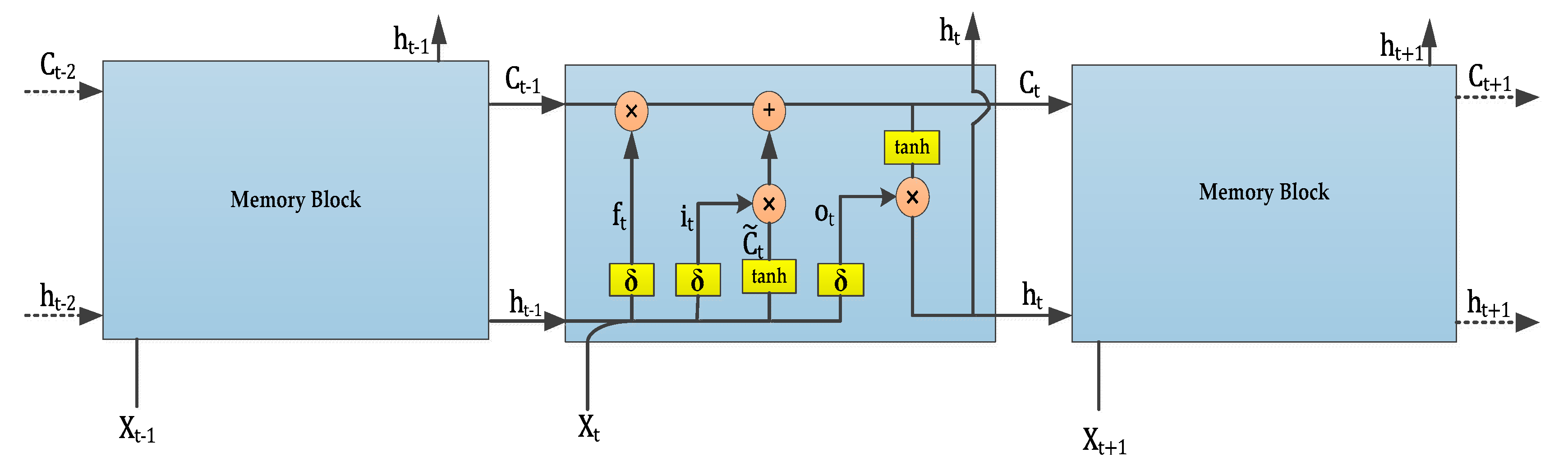
LSTM networks are a class of recurrent neural networks, in which the structure of the memory cells is modified by transforming the tanh layer in a traditional recurrent neural network into a structure containing a memory unit and a gate mechanism [20]. This mechanism determines how the information in the memory unit should be utilized and updated, thus alleviating the problem of gradient diffusion and explosion. A standard LSTM network consists of multiple memory blocks, as illustrated in Figure 1.

Each rectangular box shown in Figure 1 represents a memory block, which mainly includes a memory unit and three gates: a forget gate, an input gate and an output gate. The horizontal line at the top of the box represents the cell state, which is similar to a conveyor belt that can control the transfer of information to the next moment in time.

The first step of processing in an LSTM network is to determine what information can be passed to the cell state. This decision is controlled by the sigmoid function in the forget gate layer, which assigns a value between 0 and 1 to ${\mathrm{f}}_{\mathrm{t}}$ based on the previous output ${\mathrm{h}}_{\mathrm{t}-1}$ and the current input ${\mathrm{x}}_{\mathrm{t}}$. The value of ${\mathrm{f}}_{\mathrm{t}}$ is used to determine whether to pass on the information ${\mathrm{C}}_{\mathrm{t}-1}$ learned at the previous moment, either completely or partially [21]. The logistic sigmoid function and ${\mathrm{f}}_{\mathrm{t}}$ are expressed as follows:

$$\mathrm{sigmoid}(\mathrm{x})=\frac{1}{1+{\mathrm{e}}^{-\mathrm{x}}}$$

(14)

$${\mathrm{f}}_{\mathrm{t}}=\mathsf{\delta }({\mathrm{W}}_{\mathrm{f}}\times {\mathrm{x}}_{\mathrm{t}}+{\mathrm{U}}_{\mathrm{f}}\times {\mathrm{h}}_{\mathrm{t}-1}+{\mathrm{b}}_{\mathrm{f}})$$

(15)

where ${\mathrm{f}}_{\mathrm{t}}$ represents the forget gate and takes values in [0,1], $\mathsf{\delta }$ is the logistic sigmoid function, ${\mathrm{W}}_{\mathrm{f}}\in {\mathrm{R}}_{\mathrm{H}\times \mathrm{d}}$, ${\mathrm{U}}_{\mathrm{f}}\in {\mathrm{R}}_{\mathrm{H}\times \mathrm{H}}$, ${\mathrm{h}}_{\mathrm{t}}\in {\mathrm{R}}_{\mathrm{H}}$ and ${\mathrm{b}}_{\mathrm{f}}\in {\mathrm{R}}_{\mathrm{H}}$.

The second step is to generate the new information needed for the update. This step relies on two components: an input gate layer that uses the sigmoid function to determine which values to update and a tanh layer that generates a new candidate value ${\tilde{\mathrm{C}}}_{\mathrm{t}}$, which may be added to the cell state. We combine the values generated by these two layers to perform the update as follows:

$${\mathrm{i}}_{\mathrm{t}}=\mathsf{\delta }({\mathrm{W}}_{\mathrm{i}}\times {\mathrm{x}}_{\mathrm{t}}+{\mathrm{U}}_{\mathrm{i}}\times {\mathrm{h}}_{\mathrm{t}-1}+{\mathrm{b}}_{\mathrm{i}})$$

(16)

$${\tilde{\mathrm{C}}}_{\mathrm{t}}=\tan \mathrm{h}({\mathrm{W}}_{\mathrm{c}}\times {\mathrm{x}}_{\mathrm{t}}+{\mathrm{U}}_{\mathrm{c}}\times {\mathrm{h}}_{\mathrm{t}-1}+{\mathrm{b}}_{\mathrm{c}})$$

(17)

where ${\mathrm{i}}_{\mathrm{t}}$ represents the input gate and takes values in [0,1], ${\mathrm{W}}_{\mathrm{i}},{\mathrm{W}}_{\mathrm{c}}\in {\mathrm{R}}_{\mathrm{H}\times \mathrm{d}}$, ${\mathrm{U}}_{\mathrm{i}},{\mathrm{U}}_{\mathrm{c}}\in {\mathrm{R}}_{\mathrm{H}\times \mathrm{H}}$ and ${\mathrm{b}}_{\mathrm{i}},{\mathrm{b}}_{\mathrm{c}}\in {\mathrm{R}}_{\mathrm{H}}$.

Then, we update the old cell state. First, we multiply the old cell state by ${\mathrm{f}}_{\mathrm{t}}$ to forget the information we do not need and then add ${\mathrm{i}}_{\mathrm{t}}·{\tilde{\mathrm{C}}}_{\mathrm{t}}$ to the result to obtain the candidate value. Together, these first and second steps constitute a process of discarding unnecessary data and adding new information. Thus, ${\mathrm{C}}_{\mathrm{t}}$ is calculated as follows:

$${\mathrm{C}}_{\mathrm{t}}={\mathrm{f}}_{\mathrm{t}}\times {\mathrm{C}}_{\mathrm{t}-1}+{\mathrm{i}}_{\mathrm{t}}\times {\tilde{\mathrm{C}}}_{\mathrm{t}}$$

(18)

The final step is to determine the output of the model. An initial output is first obtained through a sigmoid layer and then the value of ${\mathrm{C}}_{\mathrm{t}}$ is scaled to the range of [−1,1] by a tanh layer; finally, the sigmoid output is multiplied pairwise with the tanh output to obtain the model output. Thus, ${\mathrm{o}}_{\mathrm{t}}$ and ${\mathrm{h}}_{\mathrm{t}}$ are obtained as follows:

$${\mathrm{o}}_{\mathrm{t}}=\mathsf{\delta }({\mathrm{W}}_{\mathrm{o}}\times {\mathrm{x}}_{\mathrm{t}}+{\mathrm{U}}_{\mathrm{o}}\times {\mathrm{h}}_{\mathrm{t}-1}+{\mathrm{b}}_{\mathrm{o}})$$

(19)

$${\mathrm{h}}_{\mathrm{t}}={\mathrm{o}}_{\mathrm{t}}\times \tan \mathrm{h}({\mathrm{C}}_{\mathrm{t}})$$

(20)

where ${\mathrm{o}}_{\mathrm{t}}$ represents the output gate and takes values in [0,1], ${\mathrm{W}}_{\mathrm{o}}\in {\mathrm{R}}_{\mathrm{H}\times \mathrm{d}}$, ${\mathrm{U}}_{\mathrm{o}}\in {\mathrm{R}}_{\mathrm{H}\times \mathrm{H}}$, ${\mathrm{h}}_{\mathrm{t}}\in {\mathrm{R}}_{\mathrm{H}}$ and ${\mathrm{b}}_{\mathrm{o}}\in {\mathrm{R}}_{\mathrm{H}}$.

Thus, the activation vector for the middle memory block at time step t is obtained. b represents the bias, we denote the memory dimensionality of the LSTM network by d and the dimensionalities of the hidden layer and input are H and h, respectively.

2.3. Microservices Architecture

This paper realized a microservices architecture by using Java and Python web technology. Network services realized by Java in the whole cluster provide the functions of assigning tasks and updating the particle swarm. The main function of multiple network services realized using Python is to calculate the fitness of multiple particles. The microservice architecture adopted in this paper is shown in Figure 2.

The Java service is implemented based on the Springboot framework, while the Python services are implemented based on the Flask framework. Different services communicate with each other through the HTTP protocol. Using Java as the service master node is intended to better extend the business-level logic in the future, while Python will focus on providing data analysis capabilities. Meanwhile, SVR and LSTM are implemented using the Python machine learning toolkits scikit-learn and TensorFlow, respectively.

2.4. PSO Algorithm

PSO is a population-based metaheuristic for global optimization [22]. The PSO algorithm solves optimization problems by means of cooperation and information sharing among the individuals in a group [23]. Suppose that there are n particles in a D-dimensional space. The position of a particle can be described by X_i = (X_i1, X_i2, X_i3, X_i4,..., X_id). The velocity of the particle can be denoted by V_i = (V_i1, V_i2, V_i3, V_i4..., V_id). Each particle has a fitness value that is determined by the objective function of the optimization problem and its best location so far (P_best) and its current location (X_i), which represents the particle’s flight experience, are known. Moreover, from the experiences of the other particles, each particle also knows the best position so far for the entire swarm (G_best), which is the best value of P_best among all particles. The velocity is updated as follows:

$${\mathrm{v}}_{\mathrm{i}}^{(\mathrm{t}+1)}={\mathsf{\omega }\mathrm{v}}_{\mathrm{i}}^{\mathrm{t}}+{\mathrm{c}}_1{\mathrm{r}}_1({\mathrm{p}}_{\mathrm{i}}-{\mathrm{x}}_{\mathrm{i}}^{\mathrm{t}})+{\mathrm{c}}_2{\mathrm{r}}_2({\mathrm{p}}_{\mathrm{g}}-{\mathrm{x}}_{\mathrm{i}}^{\mathrm{t}})$$

(21)

where ${\mathrm{x}}_{\mathrm{i}}^{\mathrm{t}}$, ${\mathrm{v}}_{\mathrm{i}}^{\mathrm{t}}$, ${\mathrm{p}}_{\mathrm{i}}$, ${\mathrm{p}}_{\mathrm{g}}$, $\mathsf{\omega }$, ${\mathrm{c}}_1$ and ${\mathrm{c}}_2$ are the current location, the current velocity, the best position in the particle’s history, the best position in the history of the entire particle swarm, an inertia weight and two learning factors, respectively. ${\mathrm{c}}_1$ and ${\mathrm{c}}_2$ are nonnegative constants that control the maximum step size; usually, ${\mathrm{c}}_1$ and ${\mathrm{c}}_2$ are usually equal to 2 because of better convergence. ${\mathrm{r}}_1$ and ${\mathrm{r}}_2$ are random numbers in the range of [0,1]. In this paper, ${\mathrm{r}}_1$ is equal to 0.6 and ${\mathrm{r}}_2$ is equal to 0.3. The location is updated as follows:

$${\mathrm{x}}_{\mathrm{i}}^{(\mathrm{t}+1)}={\mathrm{x}}_{\mathrm{i}}^{\mathrm{t}}+{\mathrm{v}}_{\mathrm{i}}^{(\mathrm{t}+1)}$$

(22)

where ${\mathrm{x}}_{\mathrm{i}}^{(\mathrm{t}+1)}$, ${\mathrm{x}}_{\mathrm{i}}^{\mathrm{t}}$ and ${\mathrm{v}}_{\mathrm{i}}^{(\mathrm{t}+1)}$ represent the position at the next moment in time, the current position and the speed at the next moment in time, respectively.

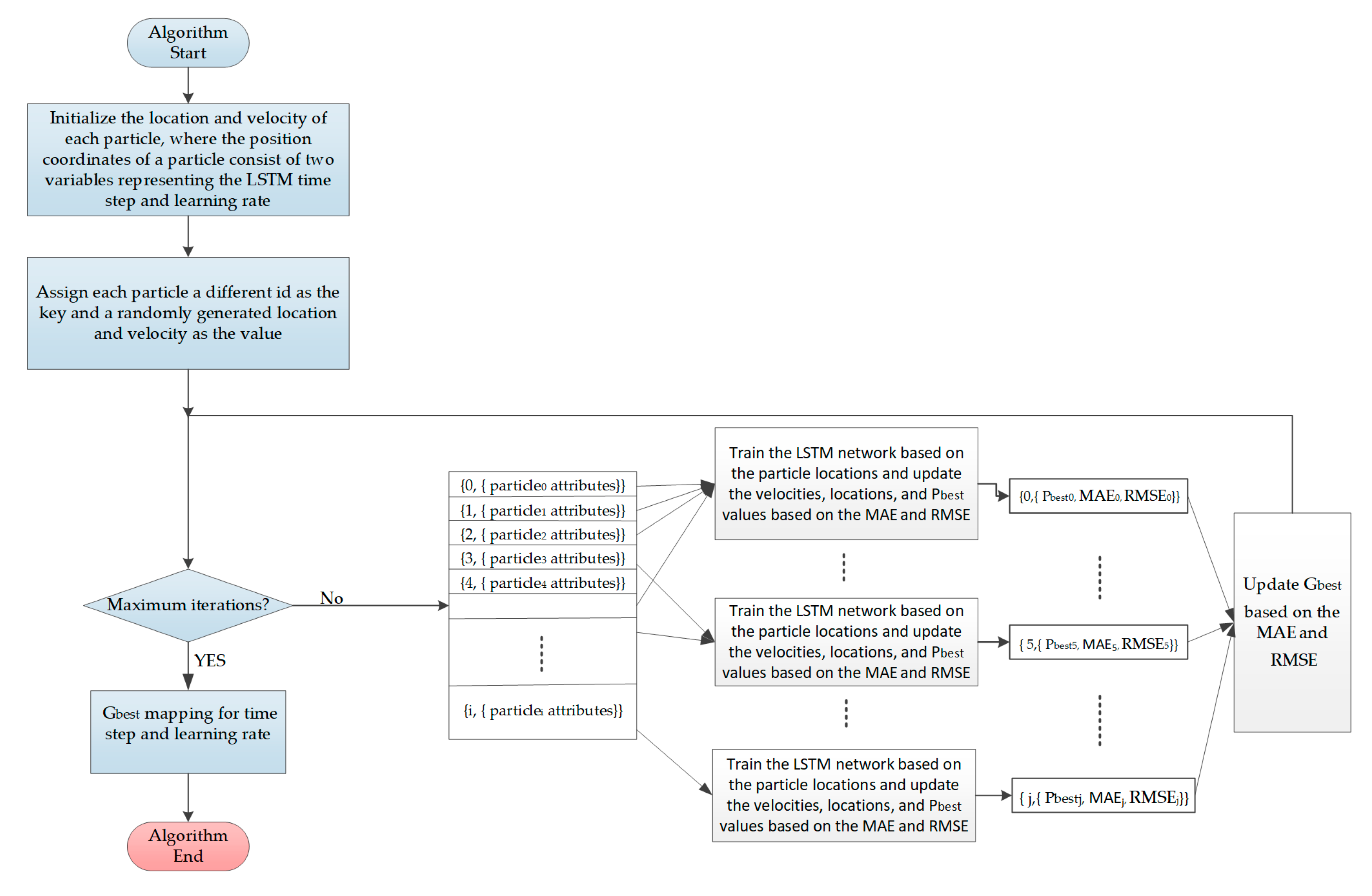
2.5. The Parallel PSO-LSTM Algorithm

In the proposed method, when the PSO algorithm is initialized, the position variable of each particle is defined as a two-dimensional variable representing the number of time steps and the learning rate of the LSTM network model. In this paper, the position and velocity of each particle are initialized as random numbers in (0,5]. The position and velocity are updated based on the average MAE and the average RMSE; PSO optimization ends when the maximum number of iterations is reached.

However, as the data volume grows and the number of particles increases, serial computing becomes inefficient. Thus, in this paper, the PSO-LSTM algorithm is parallelized via the microservices architecture.

A flowchart of the resulting parallel PSO-LSTM model for water quality forecasting is shown in Figure 3. In the parallel PSO-LSTM algorithm, the first operation is the construction of the initial particle swarm in the Java service node. Then, according to the ids of the particles, the particles are assigned to the node of the Python service for model training. Finally, the whole particle swarm is updated in the master node according to the training results of each node.

2.6. Z-score Test

Because water quality data are approximately normally distributed [4], for abnormal value detection, a Z-score test is used to identify the approximate normal distribution of the data and to find abnormal values among the numerical values of a single factor. Suppose that a value is measured multiple times with equal precision to obtain ${\mathrm{x}}_1$, ${\mathrm{x}}_2$_,..., ${\mathrm{x}}_{\mathrm{n}}$; the arithmetic average of these measurements is $\overline{\mathrm{x}}$ and the residual errors are ${\mathrm{v}}_{\mathrm{i}}={\mathrm{x}}_{\mathrm{i}}-\overline{\mathrm{x}}$ (i = 1, 2, …..., n). The standard deviation $\mathsf{\sigma }$ is calculated according to Bessel’s formula. Then, the Z-score for observation ${\mathrm{x}}_{\mathrm{i}}$ ($\left|{\mathrm{z}}_{\mathrm{i}}\right|$, 1 <= i <= n) is given as follows:

$$\left|{\mathrm{z}}_{\mathrm{i}}\right|=\left|{\mathrm{x}}_{\mathrm{i}}-\overline{\mathrm{x}}\right|/\mathsf{\sigma }$$

(23)

${\mathrm{x}}_{\mathrm{i}}$ is considered to be a poor measurement with a gross error and thus an abnormal value, if $\left|{\mathrm{z}}_{\mathrm{i}}\right|>3$ according to the Pauta criterion.

3. Development of the Method

3.1. Framework of the Method

The basic flow of the water quality data cleaning framework proposed in this study is as follows:

Step 1: Water quality data are obtained from the Gaobeidian wastewater treatment plant. Any values of the ammonia nitrogen (NH₃-N), biochemical oxygen demand (BOD), chemical oxygen demand (COD), dissolved oxygen (DO), total phosphorus (TP), total nitrogen (TN), pH, chlorides (CLS) and oil-related (OIL) quality indicators that violate logic are set as abnormal values. For example, the pH value cannot be less than 0 or greater than 14.

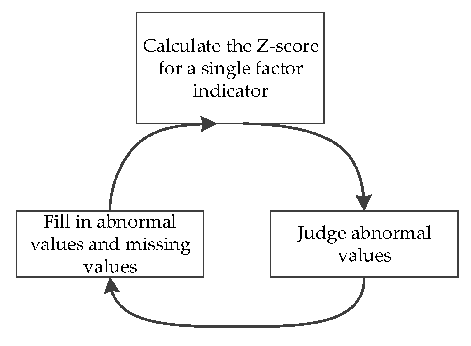
Step 2: The Z-scores for single factor indicators are calculated. Data with Z-scores greater than 3 are marked as abnormal values. Then, the total number of abnormal values and missing values in the dataset at each moment of time are counted. Any data point representing a moment in time at which the total number of abnormal values and missing values is greater than 4 is removed. For the remaining data, SVR is applied to fill in the missing values and abnormal values for each data point.

First, an available dataset for SVR is built. If there are no abnormal values or missing values for any indicators at time T_i, then the data point at time T_i is added to the available dataset. For example, suppose that for the water quality data point at time T₀, the value of COD is missing and the value of DO is abnormal. The available dataset is used to train an SVR model, with DO and COD as the outputs and the remaining indicators as the inputs. Finally, the trained SVR model is used to fill in the values of DO and COD at time T₀. That is, the values of DO and COD at time T₀ are obtained in accordance with the values of NH₃-N, BOD, TP, TN, pH, CLS and OIL at that time.

The procedures for identifying and filling in abnormal values are shown in Figure 4. Four rounds of filling in abnormal values and missing values were conducted in this study. After the last round of filling, there were almost no abnormal data.

Step 3: The parallel PSO-LSTM algorithm is used to forecast water quality indicators when all indicators are missing at a certain point in time. For example, suppose that NH₃-N, BOD, TP, TN, pH, CLS, OIL, DO and COD are all missing at time T₀. These missing indicators will be predicted based on the data of multiple moments before T₀. The validity of each model is evaluated on the basis of the MAE and RMSE.

3.2. Simple Data Analysis

The Gaobeidian wastewater treatment plant is located in Chaoyang District, Beijing Gaobeidian rural territory. It is the largest wastewater treatment plant in Beijing and the third largest wastewater treatment plant in China. Its current processing capacity is 100 million cubic meters per day. The water dataset used in this paper contains historical monitoring data from 1 July 2013 to 14 March 2016; one point of water quality data was recorded every hour. In theory, this dataset should contain 23,712 h of water quality data. In fact, however, it contains only 23,268 h of water quality data because there are 444 h of missing water quality data. This dataset contains 9 water quality indicators: TN, TP, NH₃-N, DO, pH, CLS, COD, BOD and OIL. Among the 23,268 h of data, 17,952 h of data are complete, 5316 h of data contain missing indicators. Among the initial data observations, a large number of missing data and numerical errors can be found. For example, there are many instances of continuous loss of DO data, which make it difficult to perform data mining on these water quality data. Therefore, data cleaning is necessary before water quality prediction can be performed. The data used in this paper were obtained from the Beijing Municipal Water Affairs Bureau. The statistics of the data available for each water quality indicator are presented in

Table 1. The statistics for each water indicator.

Index	TN	TP	NH3-N	DO	pH	CLS	COD	BOD	OIL
Number of data	19,946	21,117	22,001	21,680	23,131	202,09	223,20	21,779	19,785
Number of missing data	3766	2595	1711	2032	581	3503	1392	1933	3927

.

3.3. Model Evaluation Criteria

Appropriately chosen evaluation criteria are essential for assessing model performance. Because Krause has found that no single efficiency criterion can provide a full description of model performance [4] and each available criterion has certain benefits and drawbacks, we chose to apply two criteria: the MAE and the RMSE [6].

The MAE can be defined and calculated as follows:

$$\mathrm{MAE}=\frac{1}{\mathrm{n}}{\displaystyle \sum }_1^{\mathrm{n}}\left|{\mathrm{O}}_{\mathrm{i}}-{\mathrm{X}}_{\mathrm{i}}\right|$$

(24)

where ${\mathrm{O}}_{\mathrm{i}}$ and ${\mathrm{X}}_{\mathrm{i}}$ are the observed and predicted values, respectively. The MAE can effectively reflect the true prediction error in terms of the absolute deviation. The RMSE can be defined and calculated as follows:

$$\mathrm{RMSE}=\sqrt{\frac{1}{\mathrm{n}}{\displaystyle \sum }_1^{\mathrm{n}}{({\mathrm{O}}_{\mathrm{i}}-{\mathrm{X}}_{\mathrm{i}})}^2}$$

(25)

The RMSE is very sensitive to the maximum and minimum errors, which enables it to effectively reflect the accuracy of the prediction results [4]. The closer MAE and RMSE are to 0, the more accurate the prediction. This paper uses the MAE and RMSE to compare the prediction performance of different prediction models when the same dataset is used.

The mean absolute percentage error (MAPE) is used in this paper to compare the prediction performance of water time series prediction models when different datasets are used. The MAPE is defined and calculated as follows [24]:

$$\mathrm{MAPE}=100\%\times \frac{1}{n}\times {\displaystyle \sum }_1^n\frac{\left|{\mathrm{O}}_{\mathrm{i}}-{\mathrm{X}}_{\mathrm{i}}\right|}{{\mathrm{O}}_{\mathrm{i}}}$$

(26)

The MAPE not only considers the error between the predicted value and the true value but also considers the ratio between the error and the true value.

4. Results and Discussion

First, the values of the NH₃-N, BOD, COD, DO, TP, TN, pH, CLS and OIL indicators that violate logic are marked as abnormal values. Then, the Z-scores are calculated for each water quality indicator to identify abnormal values. The statistics for the number of abnormal values plus the number of missing values are shown in

Table 2. Statistics for the number of abnormal values plus the number of missing values.

Index	Equal to 1	Equal to 2	Equal to 3	Equal to 4	Greater than 4
Data proportion	78%	12%	8%	1%	1%

. As illustrated in Table 2, the water quality data points are categorized into those for which the total number of abnormal values plus missing values is one, two, three, four or more than four. In this paper, it is considered that the data prediction error will be higher when more values are missing. In addition, the data points for which the total number of abnormal values and missing values is less than or equal to four times account for 99% of the dataset. Therefore, SVR is used only in these cases. The remaining 1% of the data are removed from the dataset. After removal, this dataset contains 23,036 h of data to be subjected to SVR processing. The SVR model is used to fill in the abnormal and missing values of each single factor indicator.

Table 3. The number of abnormal values of each water indicator.

Index	TN	TP	NH3-N	DO	pH	CLS	COD	BOD	OIL
Before filling	213	197	177	189	179	202	200	169	202
First round of filling	24	31	19	37	34	20	20	23	20
Second round of filling	6	7	4	11	13	7	9	8	10
Third round of filling	1	0	0	0	1	1	0	0	2
Fourth round of filling	1	0	0	0	1	1	0	0	1

shows the numbers of abnormal values of the water quality indicators before and after filling. As illustrated in Table 3, to reduce the possibility of errors in data analysis, the SVR algorithm can be used to reduce the impact of abnormal and missing values on subsequent water quality analyses. As the number of abnormal values decreases, the training accuracy of the LSTM networks can be greatly increased. Especially in the case of a large increase in the amount of data collected in the future, a correspondingly large number of abnormal values could make it difficult to train an accurate model.

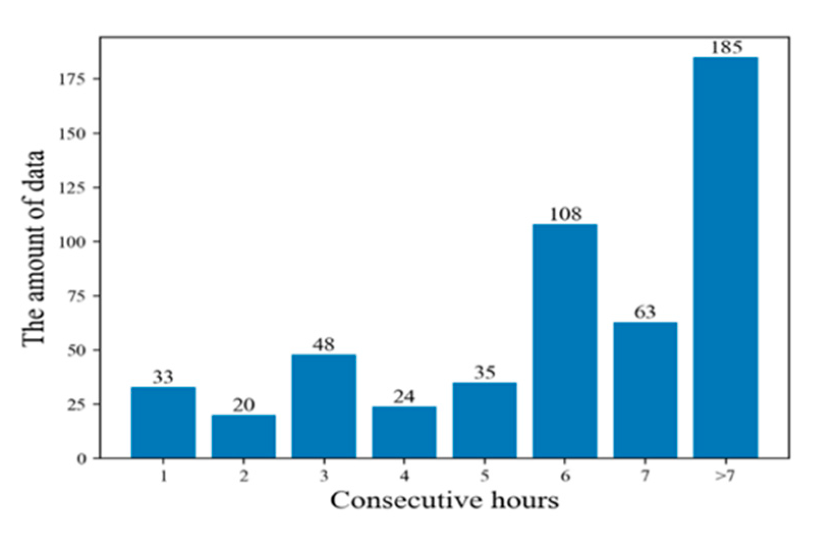
After the above analysis, a dataset without outliers was obtained. Through the analysis of the time series, it was found that there were still 676 time points in the data set for which all water quality indicators were missing. Before establishing the parallel PSO-LSTM model to predict the time series, this paper analyzes the features of consecutive missing data in this dataset, as shown in Figure 5. As illustrated in Figure 5, separate counts are presented for segments of continuous missing data of different durations, including 1 consecutive hour, 2 consecutive hours, 3 consecutive hours, 4 consecutive hours, 5 consecutive hours, 6 consecutive hours, 7 consecutive hours and more than 7 consecutive hours. The distribution of missing data is clearly random. For example, data missing for 2 consecutive time points happened just ten times, so in Figure 5, when the number of consecutive hours is equal to 2, the amount of data is 20.

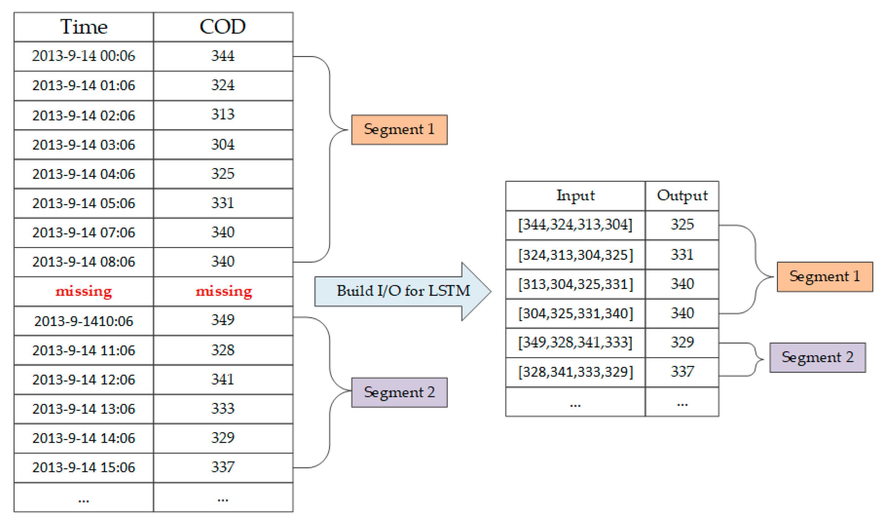
Considering the distribution of the missing data, segments of data for which the water indicators can be obtained for at least 30 consecutive hours are regarded as available for training and testing. For example, there are 1920 consecutive hours of data from 1 July 2013, to 18 September 2013 in this dataset. Therefore, these data can be added to the available dataset. Once the available dataset has been constructed, these data are used as testing data and training data for the LSTM networks to construct a predictive model for past time series to be used in predicting future time series. The shortest consecutive segment that has values in the available dataset has a duration of 30 h and the longest has a duration of 3312 h. Thus, the available dataset consists of multiple segments of data that are continuously distributed over time. Taking the COD time series as an example, it is assumed that the timesteps of LSTM network are equal to 4 to construct the input and output datasets. The process is shown in Figure 6. Other water quality indicators are also predicted by building data sets in this manner.

In the parallel PSO-LSTM model, the position variable of each particle is defined as a two-dimensional variable representing the value of time steps and the learning rate of the LSTM network model and the position and velocity of each particle are initialized as random numbers in (0,5] at the start of the PSO algorithm. Particles are assigned to hosts in the cluster based on their id values and will be updated.

The following experiment takes the process of predicting the COD value as an example. In this experiment, the maximum number of PSO iterations is 160, the number of particles in the particle swarm is 100, the number of hidden layer neurons in the LSTM network is 120 and the ratio of the training set to the test set is 8:2. As illustrated in

Table 4. Iterative results of using PSO to predict chemical oxygen demand (COD).

PSO Iterations	Time Steps	Learning Rate	MAE	RMSE
20	4	0.781033	154.25	176.63
40	4	0.197025	94.80	110.27
60	4	0.098331	76.21	87.58
80	4	0.002876	72.84	83.12
100	3	0.003004	48.99	56.84
120	4	0.002904	39.44	45.63
140	4	0.002876	22.52	25.79
160	4	0.002876	20.05	23.11

, as the number of iterations increases, the values of the LSTM network parameters come closer to optimality. As illustrated in Table 4, when the learning rate of the LSTM networks equal to 0.002876 and the number of timesteps is equal to 4, it is most accurate to predict COD at the next moment by using the values of the first four moments.

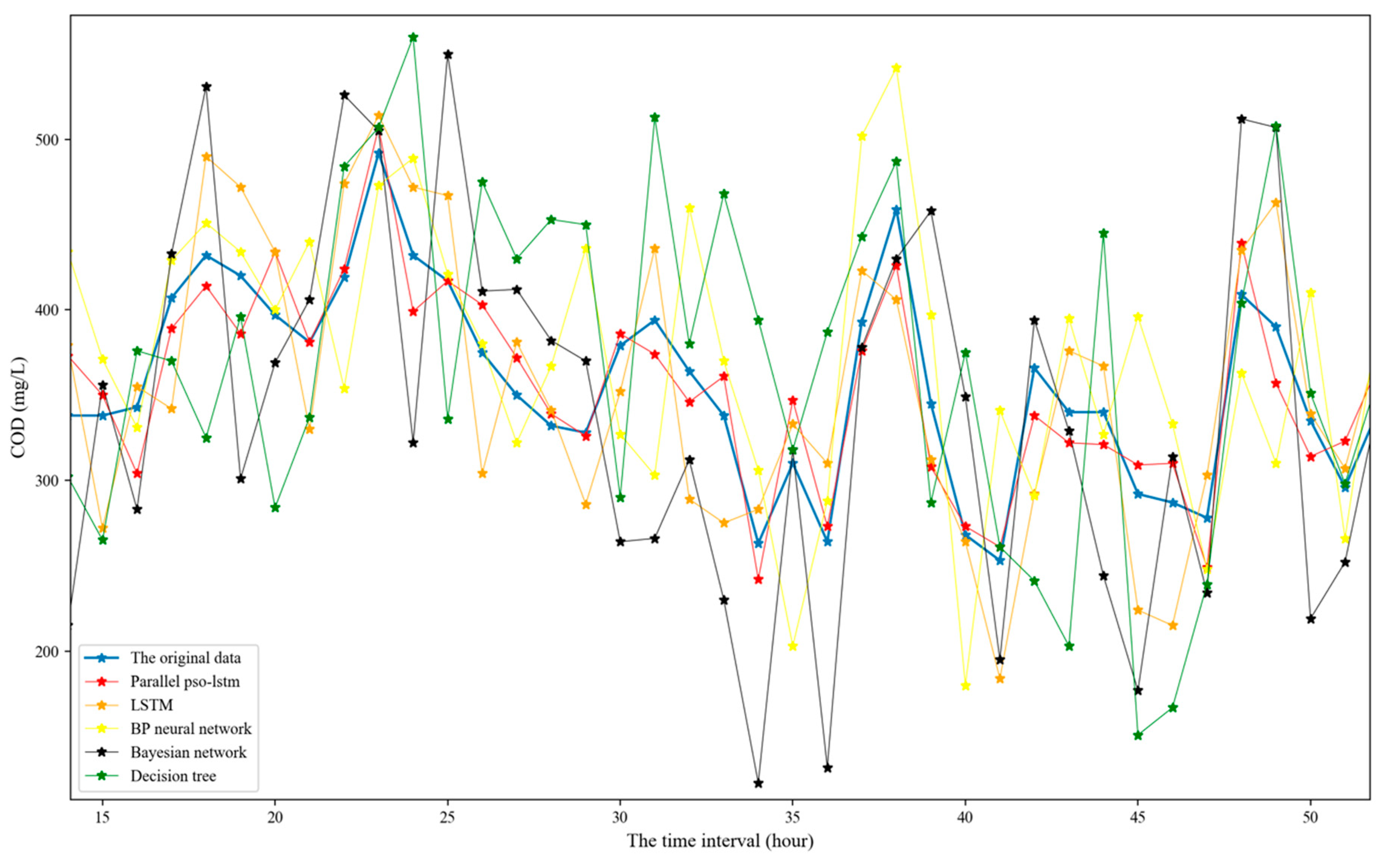
The performance of the parallel PSO-LSTM model is presented in

Table 5. Accuracy comparison of the PSO-LSTM model and other machine learning models.

Index	Optimized LSTM	LSTM	BP Neural Network	Bayesian Network	Decision Tree
MAE	20.05	39.25	61.83	80.62	91.06
RMSE	23.11	44.56	53.88	68.19	78.4

along with the performance results of four other models for comparison. In this experiment, other machine learning models are also used to build training and test sets using 4 time steps. As illustrated in Table 5, the optimized LSTM network model achieves better prediction accuracy, especially when compared to the Bayesian network model. Figure 7 shows the prediction of COD time series using each model for 40 moments in time. As illustrated in Figure 7, when PSO-LSTM is used to predict water quality time series, the results are closest to the original data, so this model is the most accurate.

As illustrated in

Table 6. Time consumption comparison of parallel and serial PSO-LSTM implementations.

PSO Iterations	Serial PSO-LSTM Time (s)	Parallel PSO-LSTM Time (s)
20	160.88	53.33
40	330.73	118.27
60	510.78	180.12
80	809.54	282.84
100	1213.79	404.69
120	1410.88	479.34
140	1702.58	583.42
160	2013.64	701.82

, the microservices architecture implementation greatly improves the program execution efficiency of the prediction model compared to that of a PSO-LSTM model with a serial implementation. The table compares the experimental findings with regard to the time taken to complete various numbers of PSO iterations for the serial and parallel implementation of the PSO-LSTM algorithm.

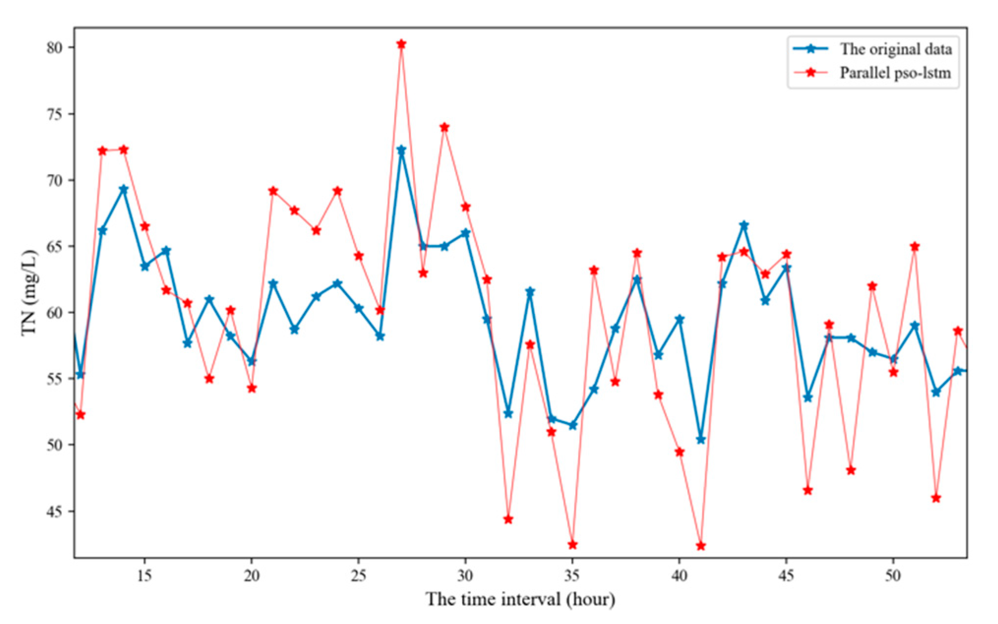
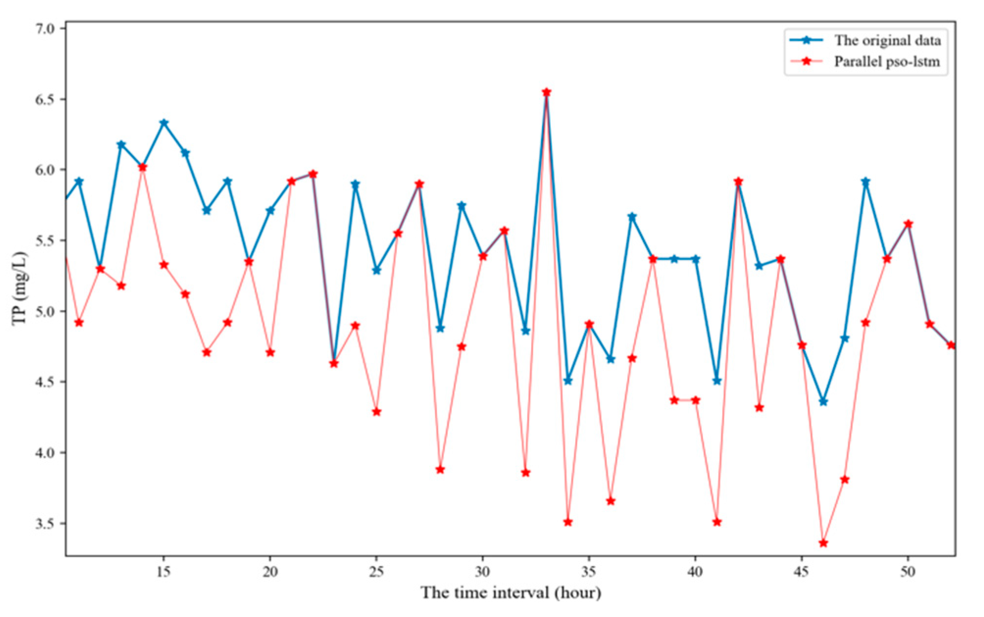
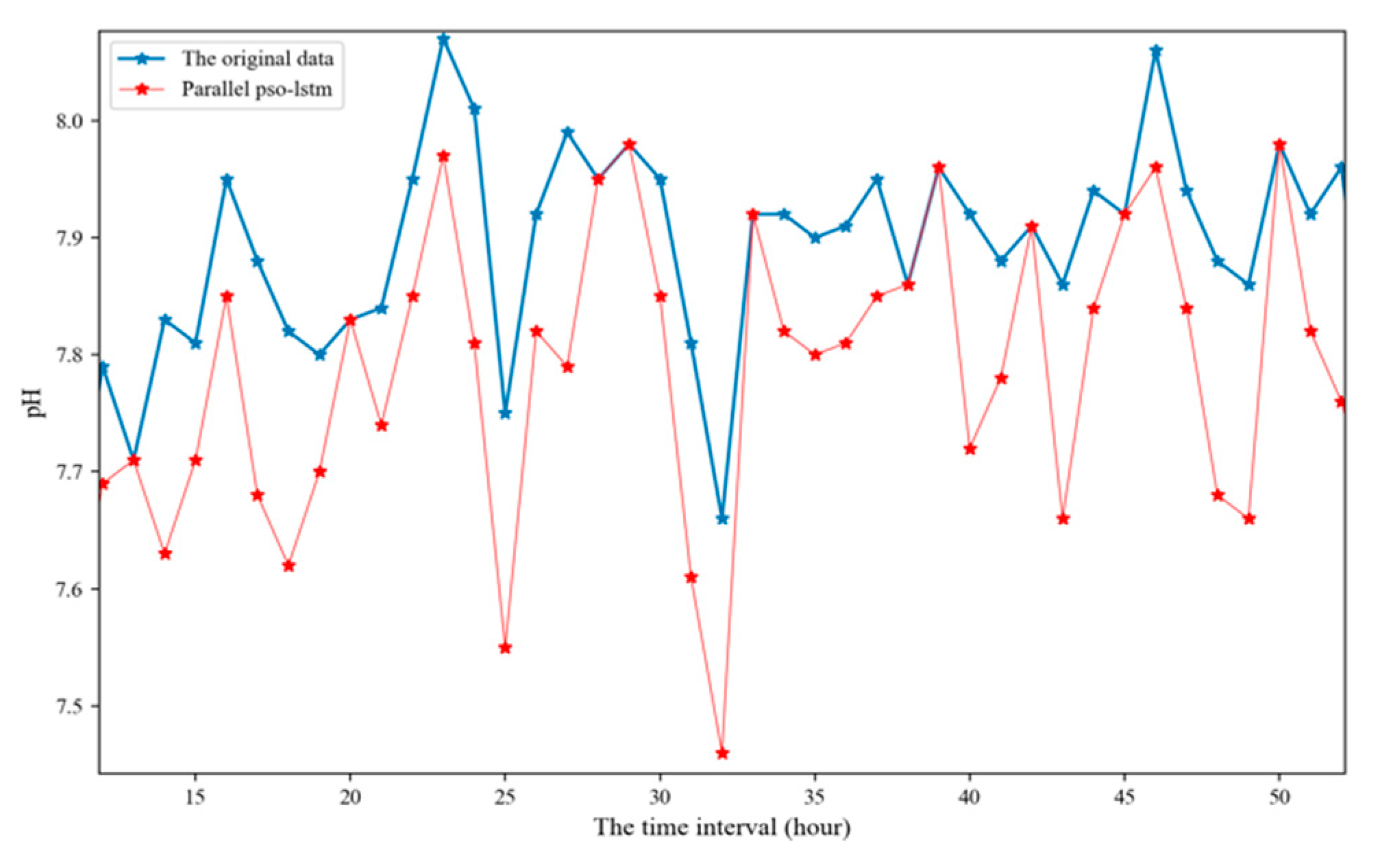
This paper uses the PSO-LSTM model trained in the above experiment to predict the TN, TP and pH values. As shown in Figure 8, Figure 9 and Figure 10 and

Table 7. Accuracy of the PSO-LSTM model.

Index	TN	TP	pH
MAE	4.89	0.45	0.76
RMSE	5.62	0.67	0.87

, this model has a good prediction performance for water quality time series prediction.

To further illustrate that the PSO-LSTM model used in this paper has higher accuracy in predicting water quality time series, this paper compares it with the prediction results of literature [24], who used a hybrid optimized BP network model to predict dissolved oxygen time series. The results are reported in

Table 8. Accuracy of the water quality time series prediction models.

	Index	MAPE
literature [24]	dissolved oxygen	6.7219
PSO-LSTM	COD	5.3845
PSO-LSTM	TN	7.0321
PSO-LSTM	TP	5.9364
PSO-LSTM	pH	6.3451

. As indicated in Table 8, the PSO-LSTM model used in this paper generally has a smaller MAPE value, which indicates a good performance at predicting water quality time series.

5. Conclusions

With continuously increasing demand for prediction accuracy and efficiency, the complexity of algorithms is also increasing; moreover, the amount of abnormal and missing values is growing, leading to challenges in water quality analysis. To satisfy the need for water quality data of high integrity and accuracy, a framework for water data cleaning of time series data is proposed in this paper. First, a Z-score test is used to identify abnormal values and an SVR algorithm is used to fill in abnormal and missing values. The PSO algorithm is used to optimize the selection of the parameters for LSTM networks. To reduce the model execution time in a complex computing environment, a parallel implementation of the PSO-LSTM algorithm is realized based on a microservices architecture. In addition, the MAE and RMSE are used to evaluate the performance of the prediction model. Experiments based on data from the Gaobeidian wastewater treatment plant have verified the effectiveness of the presented model.

The experimental results presented in Section 4 show that the proposed parallel PSO-LSTM method can provide accurate predictions and analytics regarding comprehensive water quality and it can also perform increasingly complex computations in less time than standalone serial algorithms. This model can be applied to forecasting and cleaning for any datasets similar to water quality time series data; thus, this model has widespread application potential. Moreover, this study is valuable as a reference for water quality forecasting. The results of this study promote the application of machine learning algorithms to water quality prediction and the predicted results can guide decisions for future water management. The framework proposed in this paper can be used as a general model for cleaning time series data.

Based on the models proposed in this paper, further work will proceed as follows. The PSO algorithm has a certain blindness and randomness; these shortcomings need to be studied and solved in the future to determine the most appropriate value of the inertia weight used in this algorithm. Future studies should further investigate the correlations of time series data in the time dimension to fill in outliers more accurately. In addition, the communication between clusters uses the HTTP protocol, while the HTTP protocol is a text protocol, so a large amount of bandwidth is wasted. More efficient binary protocols should be studied in the future.

References

- Guo, H.; Jeong, K.; Lim, J.; Jo, J.; Kim, Y.M.; Park, J.-P.; Kim, J.H.; Cho, K.H. Prediction of effluent concentration in a wastewater treatment plant using machine learning models. J. Environ. Sci. 2015, 32, 90–101. [Google Scholar] [CrossRef]
- Wu, J.; Xu, S.; Zhou, R.; Qin, Y. Scenario analysis of mine water inrush hazard using Bayesian networks. Saf. Sci. 2016, 89, 231–239. [Google Scholar] [CrossRef]
- Bagriacik, A.; Davidson, R.A.; Hughes, M.W.; Bradley, B.A.; Cubrinovski, M. Comparison of statistical and machine learning approaches to modeling earthquake damage to water pipelines. Soil Dyn. Earthq. Eng. 2018, 112, 76–88. [Google Scholar] [CrossRef]
- Zhang, L.; Zou, Z.; Shan, W. Development of a method for comprehensive water quality forecasting and its application in Miyun reservoir of Beijing, China. J. Environ. Sci. 2017, 56, 240–246. [Google Scholar] [CrossRef]
- Gonzalez, J.; Yu, W. Non-linear system modeling using LSTM neural networks. IFAC-PapersOnLine 2018, 51, 485–489. [Google Scholar]
- Zhou, J.; Wang, Y.; Xiao, F.; Wang, Y.; Sun, L. Water Quality Prediction Method Based on IGRA and LSTM. Water 2018, 10, 1148. [Google Scholar] [CrossRef]
- Liang, C.; Li, H.; Lei, M.; Du, A.Q. Dongting Lake Water Level Forecast and Its Relationship with the Three Gorges Dam Based on a Long Short-Term Memory Network. Water 2018, 10, 1389. [Google Scholar] [CrossRef]
- Yan, J.Z.; Chen, X.Y.; Yu, Y.C. A Data Cleaning Framework for Water Quality Based on NLDIW-PSO Based Optimal SVR. In Proceedings of the IEEE/WIC/ACM International Conference on Web Intelligence (WI), Santiago, Chile, 3–6 December 2018. [Google Scholar]
- Gambhir, S.; Malik, S.K.; Kumar, Y. PSO-ANN based diagnostic model for the early detection of dengue disease. New Horizons Transl. Med. 2017, 4, 1–8. [Google Scholar] [CrossRef]
- Muhammad, A.; Waheed, I.; Abdelkarim, E. Unsupervised learning approach for web application auto-decomposition into microservices. J. Syst. Softw. 2019, 151, 243–257. [Google Scholar]
- Schmidt, M.; Obermaisser, R. Adaptive and technology-independent architecture for fault-tolerant distributed AAL solutions. Comput. Boil. Med. 2018, 95, 236–247. [Google Scholar] [CrossRef]
- Philippe, R.; Marc, D.; Christina, H.; Kyle, R. KaliGreen: A distributed Scheduler for Energy Saving. Procedia Comput. Sci. 2018, 141, 223–230. [Google Scholar]
- Zhang, X.G. Introduction to Statistical Learning Theory and Support Vector Machines. Acta Autom. Sinica 2000, 26, 32–42. [Google Scholar]
- Chen, K.-Y. Forecasting systems reliability based on support vector regression with genetic algorithms. Reliab. Eng. Syst. Saf. 2007, 92, 423–432. [Google Scholar] [CrossRef]
- Li, Z.B.; Niu, B.S.; Peng, F.; Li, G.; Yang, Z.; Wu, J. Classification of Peanut Images Based on Multi-features and SVM. IFAC-PapersOnLine 2018, 51, 726–731. [Google Scholar] [CrossRef]
- Luo, Y.G.; Xiong, Z.Y.; Xia, S.Y.; Tan, H.J.; Gou, J.P. Classification noise detection based SMO algorithm. Optik 2016, 127, 7021–7029. [Google Scholar] [CrossRef]
- Rastogi, R.; Pal, A.; Chanra, S. Generalized Pinball Loss SVMs. Neurocomputing 2018, 322, 151–165. [Google Scholar] [CrossRef]
- Jiang, H.; Ching, W.-K.; Yiu, K.F.C.; Qiu, Y. Stationary Mahalanobis kernel SVM for credit risk evaluation. Appl. Soft Comput. 2018, 71, 407–417. [Google Scholar] [CrossRef]
- Zhou, T.; Lu, H.L.; Wang, W.W.; Yong, X. GA-SVM based feature selection and parameter optimization in hospitalization expense modeling. Appl. Soft Comput. 2019, 75, 323–332. [Google Scholar]
- Xu, P.; Du, R.; Zhang, Z.B. Predicting pipeline leakage in petrochemical system through GAN and LSTM. Knowl. Based Syst. 2019, 175, 50–61. [Google Scholar] [CrossRef]
- Zhou, T.; Lu, H.L.; Wang, W.W.; Yong, X. Learning document representation via topic-enhanced LSTM model. Knowl. Based Syst. 2019, 174, 194–204. [Google Scholar]
- Hauduc, H.; Neumann, M.B.; Muschalla, D.; Gamerith, V.; Gillot, S.; Vanrolleghem, P.A. Efficiency criteria for environmental model quality assessment: A review and its application to wastewater treatment. Environ. Model. Softw. 2015, 68, 196–204. [Google Scholar] [CrossRef]
- Adel, M.; Farhang, S.; Mohammad, A. Overbreak prediction in underground excavations using hybrid ANFIS-PSO model. Tunn. Undergr. Space Technol. 2018, 80, 1–9. [Google Scholar]
- Yan, J.Z.; Xu, Z.B.; Yu, Y.C.; Xu, H.X.; Gao, K.L. Application of a Hybrid Optimized BP Network Model to Estimate Water Quality Parameters of Beihai Lake in Beijing. Appl. Sci. 2019, 9, 1863. [Google Scholar] [CrossRef]
Figure 1.
Basic structure of a long short term memory (LSTM) network.
Figure 2.
Microservices architecture used in this paper.
Figure 3.
Flowchart of the parallel particle swarm optimization- long short term memory (PSO-LSTM) model for water quality forecasting.
Figure 4.
The procedures for preprocessing abnormal values.
Figure 5.
Statistics of segments of continuous missing data.
Figure 6.
The process of building the input and output datasets for LSTM networks.
Figure 7.
The prediction of COD time series using each model for 40 moments in time.
Figure 8.
The prediction of total nitrogen (TN) time series using parallel PSO-LSTM model for 40 moments in time.
Figure 9.
The prediction of total phosphorus (TP) time series using parallel PSO-LSTM model for 40 moments in time.
Figure 10.
The prediction of pH time series using parallel PSO-LSTM model for 40 moments in time.