The Role of Hydraulic Hysteresis on the Hydrological Response of Pyroclastic Silty Covers


1
REgional Models and Geo-Hydrological Impacts, Fondazione CMCC Centro Euro-Mediterraneo sui Cambiamenti Climatici, 81043 Capua (CE), Italy
2
Dipartimento di Ingegneria, Università della Campania “Luigi Vanvitelli”, 81031 Aversa (CE), Italy
3
Dipartimento di Ingegneria Civile Edile e Ambientale, Università di Napoli “Federico II”, 80125 Napoli, Italy
*
Author to whom correspondence should be addressed.
Water 2019, 11(3), 628; https://doi.org/10.3390/w11030628
Submission received: 15 February 2019
/
Revised: 13 March 2019
/
Accepted: 22 March 2019
/
Published: 26 March 2019
(This article belongs to the Special Issue The Role of Water in Shallow and Deep Landslides)
Abstract
:A significant part of the recent geotechnical literature concerning pyroclastic soils is focused on the characterization of the hydrological effects of precipitations and their implications for the stability conditions of unsaturated sloping covers. Recent experience shows that suction-induced strength reduction is influenced by various factors including hydraulic hysteresis. A deeper insight into the hysteretic water retention behavior of these materials and its effects upon their response to dry/wetting conditions is a major goal of this paper, which exploits the data provided by the monitoring of a volcanic ash. Based on the parameters retrieved from data calibration, the hydrological response of a virtual slope subject to one-dimensional rainfall infiltration is investigated by numerical analyses and compared with the results obtained through the usually adopted non-hysteretic approaches. The analysis demonstrates that considering the hysteretic behavior may be crucial for a proper evaluation of the conditions leading to slope failure.
1. Introduction
Unsaturated pyroclastic silty covers, widely spread in the world, are often involved in disastrous landslides ([1]; NatCatServices datasets). Precipitation-induced suction drops may in fact lead to a significant reduction in safety conditions up to the landslide triggering.
Landslide events that occurred in the last decades in the Campania region, Southern Italy, confirm these considerations [2,3,4,5,6,7]. After those events, a great research effort has gone into systematic field and laboratory studies. These allowed the collection of a lot of data regarding soil properties [8,9], the hydrological processes of infiltration and evapotranspiration [3,10,11,12,13], failure processes, and subsequent propagation [14,15].
Investigations and research activities have allowed outlining of the characteristics of the rainfall events which can lead to slope failure in pyroclastic silty soils [2,3]; these rainfall event characteristics can differ from those affecting the stability of coarse-grained and fine-grained soils. Specifically, short rainfall events primarily affect the behavior of slopes in coarse-grained soils; on the contrary, slopes in fine-grained soils may fail under the effects of prolonged wet periods lasting even an entire hydrological year while single intense events play a minor role [4]. Silty pyroclastic soils display an intermediate response, depending on both wet antecedent conditions and single rainfall events.
Such studies have clearly demonstrated that the influence of the antecedent meteorological history on stability conditions must be related to the large amount of water that may be absorbed and retained. This depends on the small interparticle pores present in the silty fraction, which can retain the liquid phase, and on the high soil porosity, which allows storage of water.
The same studies have shown that the hysteretic hydraulic soil response can affect the s–θ (suction–water content) distribution at the beginning of critical rainfall events, with permeability and volumetric water content of soils at a given suction on a wetting path having a lower value than those on the corresponding drying path. In this regard, it is possible to identify the drying (or desorption) boundary curve and wetting (or adsorption) boundary curve, and the primary drying (wetting) curves due to the drying (wetting) processes starting from the wetting (drying) boundary curve up to further fluctuation of drying and wetting states formed during scanning. In this way, the initial conditions are hardly foreseeable, being a combined effect of the previous weather forcing history and the hysteretic soil response.
The hysteretic response of pyroclastic soils has been recently documented through a systematic comparison between pairs of volumetric water content and matric suction measurements made at the same depths in two instrumented slopes in the Campania region (Monterforte Irpino [16] and Cervinara [17]). These data, which lay below the main laboratory drying curve, show distinct paths along scanning curves which, in turn, do not seem to exhibit a significant internal hysteresis. Basile et al. [18] report similar data by a comparison between laboratory and field data coming from the alluvial plain of Piano Campano (Campania region). Based on experience accumulated in the regional context, recently, Comegna et al. [19] have investigated the influence of potential wetting paths on virtual slope stability conditions, stressing the potential errors in the prediction of landslide triggering, which might be associated with the use of a unique soil–water characteristic curve (SWCC), which is usually assumed to simplify the wetting paths. In particular, along scanning curves, they have highlighted that a quicker water content change than found in other paths could take place; therefore, under critical precipitation the time to failure could be shorter than expected.
Within this framework, this paper attempts to improve the understanding about how hysteretic dynamics can influence the soil hydraulic behavior and the slope response of silty pyroclastic covers. Such insights should be taken into account when predictive tools for early warning systems have to be developed. To this aim, the paper is articulated into the following parts:
- investigation of the wetting/drying paths of an instrumented reconstituted ash layer exposed to weather forcing over four consecutive years;
- selection of a suitable model for analysis of the hydraulic hysteresis and calibration of the parameters required to simulate the soil behavior;
- analysis of the role of the hydraulic hysteresis of a virtual slope in response to a critical event, and comparison with the results obtained by the usual non-hysteretic approaches.
2. Materials and Methods
2.1. Test Device and Investigated Soil
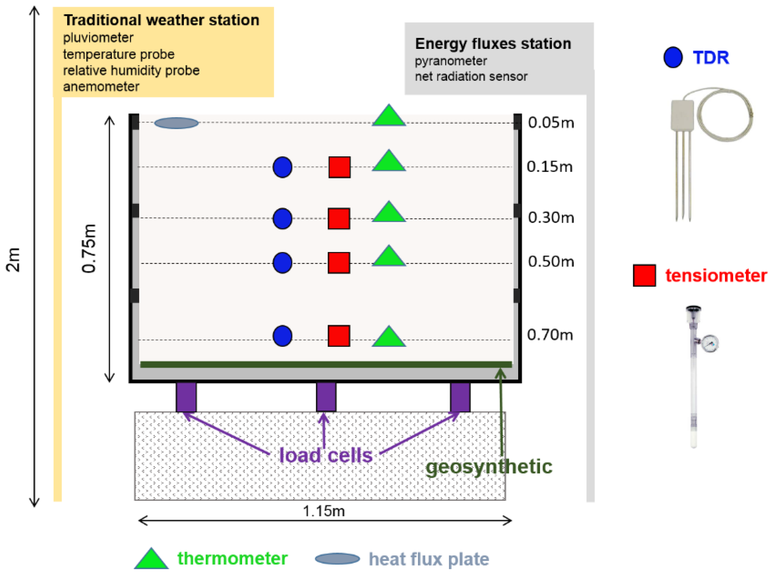
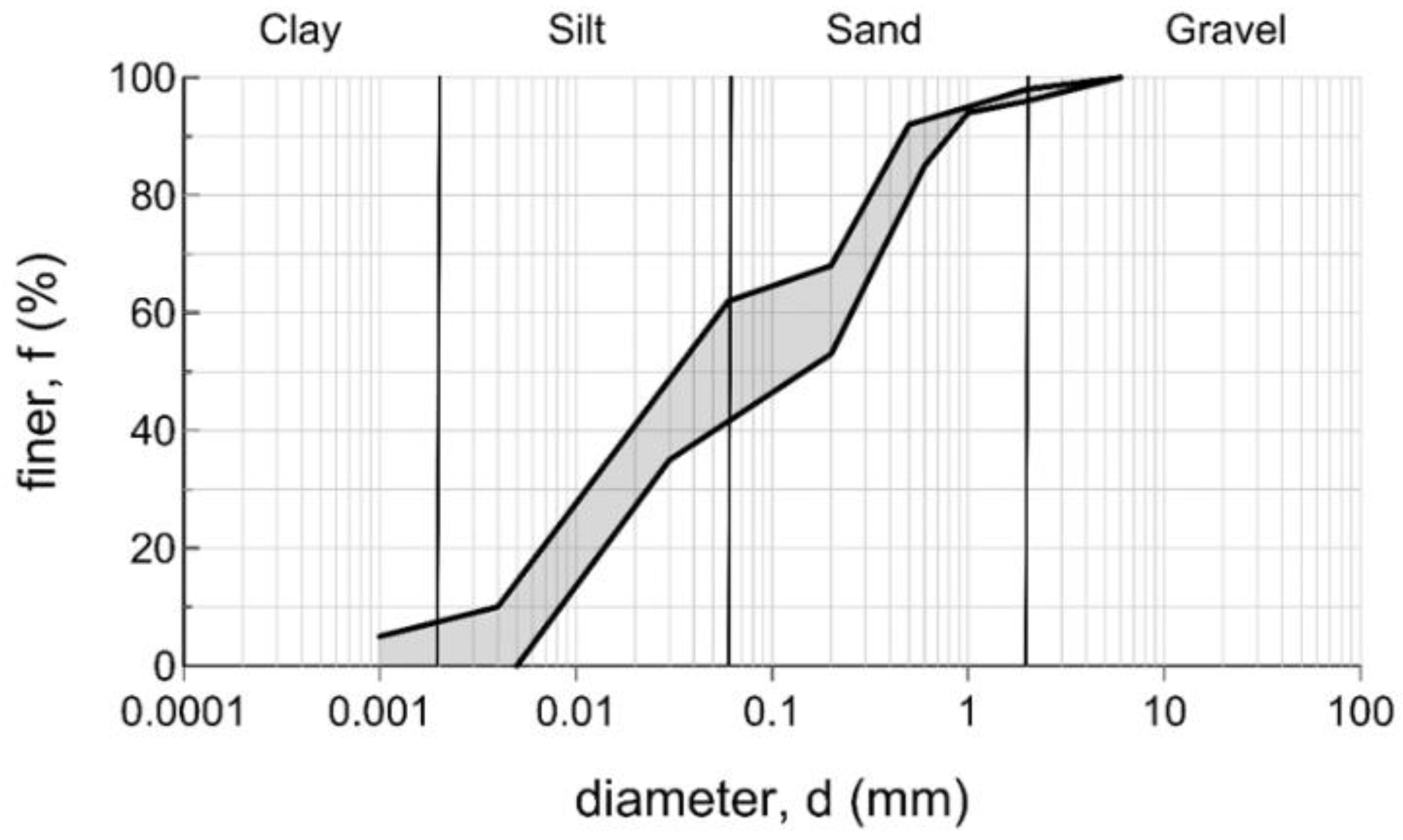
An accurate and targeted investigation of the considered subject was performed by systematic measurements of suction and of water content in an instrumented lysimeter (Figure 1) consisting of a wooden tank of about 1 m3 (height 75 cm, surface area 1.3 m2) [12]. It was located in Naples and studied with weather forcing comparable to that usually experienced by slopes composed of the same materials that are potentially affected by landslide events in Campania. Monteforte Irpino ash [16] was laid down in the lysimeter. Such a material was produced in the last 10,000 years by the volcanic centre of Somma-Vesuvius. The finest component of the soil (a silt with some clay, Figure 2) was non-plastic due to the absence of active minerals. The field porosity was as high as 70% with peaks attaining 80%. The layer was put in place by means of dry pluvial deposition at the same field porosity (70%) and exposed to the atmosphere for several hydrological years. Specifically, during the timespan of September 2010–August 2014, the soil surface was left bare to reduce the complexity of the involved dynamics and the generated data was used for analysis. A geotextile sheet was placed at the bottom of the soil layer. In that investigation, a weather station monitored the atmospheric variables. Rainfall infiltration and evaporative fluxes were obtained by regularly weighing the tank through three load cells. The evaporative flux was also indirectly obtained by measuring the different water energetic terms at the soil–atmosphere interface. The hydrological variables, suction (s) and volumetric water content (θ), were monitored at four different depths (at 15, 30, 50, and 70 cm) using jet-fill tensiometers and time domain reflectometry (TDR) probes.
2.2. Modeling Approaches
The effects of the rainwater infiltration are commonly investigated through the Richards [20] equation. For one-dimensional vertical flow, this can be written as:
where t is time, z the spatial coordinate, k(θ(s)) the hydraulic conductivity function (HCF), and γw the unit weight of water. The use of such an equation requires soil characterization through both the SWCC and the hydraulic conductivity function (HCF).
One of the most popular expressions for the SWCC is the well-known empirical equation proposed by van Genuchten [21]:
where Se is the so-called “effective saturation degree”, θs and θr the saturated and the residual volumetric water content of the soil, and n and α (kPa−1) are two empirical parameters.
The HCF is instead usually defined through the equation proposed by Mualem [22] in combination with the van Genuchten SWCC:
where k and ks represent the current and the saturated hydraulic conductivity, respectively.
In order to account for the hydraulic hysteresis, the SWCC and the HCF should be properly modified [23,24,25]. In this paper the model proposed by Parker and Lenhard [26] was adopted, here indicated as the PL model.
According to this model, the wetting and drying scanning curves of the SWCC can be obtained by scaling the correspondent main curves defined by the van Genuchten equation. In particular, the residual water content and the coefficient n of these two curves coincide (θr = θrw = θrd; nw = nd = n); the differences concern only the values of the saturated volumetric water content (θsd being higher than θsw) and of the coefficient α (αd being less than αw). Compared to other models based on a scaling procedure [27,28], the PL model allows prevention of the artificial pumping error, that is, the non-closure of the scanning loops in simulated cyclic paths, which is considered to be an aberration rather than a soil property [29]. This is avoided by collecting all the reversal points experienced by the soil. Preserving the “memory” of the various wetting–drying cycles to which they have been subjected allows paths to draw closed scanning loops.
A wetting scanning path starting from a point (sΔdw, SeΔdw) located on a main or a scanning curve and ending at a wetting-to-drying turn point is expressed by the following equation:
where Sew is the effective saturation degree calculated with the van Genuchten equation (Equation (2)) for the main wetting curve; sΔdw, SeΔdw are the s and Se values corresponding to the starting drying-to-wetting turn point; and sΔwd and SeΔwd are the values corresponding to the wetting-to-drying turn point.
Conversely, a drying scanning path starting from a wetting-to-drying reversal point having the coordinates (sΔwd, SeΔwd) and ending at a drying-to-wetting reversal point (sΔdw, SeΔdw) is expressed by the similar equation:
where Sed is the effective saturation calculated by the van Genuchten equation (Equation (2)) with (θsd, θr, αd, n) parameters.
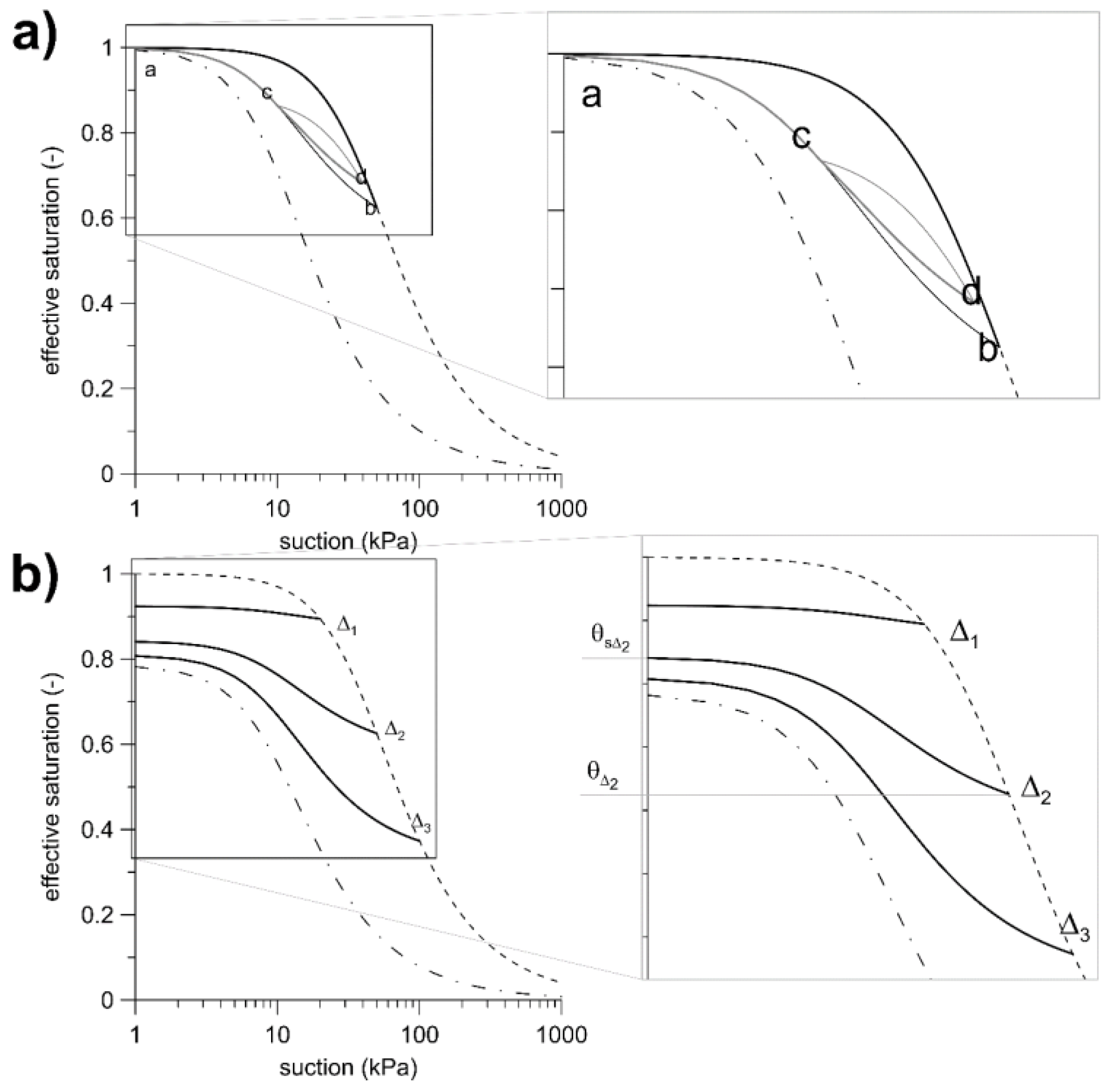
An example is illustrated in Figure 3a in the Se–s plan where, for sake of simplicity, the ideal condition of a closed main hysteresis loop at saturation (neglecting air entrapment) is assumed. The initial soil state is represented by point a (θsd = θsw) corresponding to a condition close to full saturation. A first desaturation process is supposed to follow the main drying curve up to point b. The subsequent wetting path would lead the soil state from b to c along the curve obtained by scaling the main wetting curve in such a way to pass through the reversal points a and b. A further hypothetical drying path c–d is obtained by scaling the main drying curve which, in this case, should pass through the reversal points b and c. The final wetting path d–a is defined by scaling the main wetting curve again, which moves through the points a, c, and d.
Following the Land approach [30], the PL model may account for the air entrapment effect assuming that, in a wetting/scanning path starting from a turning point Δ towards the zero suction value, the difference R between the reciprocal of the difference between the initial and final volumetric water contents is constant (Figure 3b):
In this expression, θ∆ is the water content at the reversal point Δ and θs∆ is the water content achieved for null suction starting from Δ. The minimum value of θs∆ is θsw, which is obtained by assuming θ∆ = θr.
Moving to the permeability function, HCF, it is worth to notice that the PL model adopts the Mualem–Van Genuchten equation. Consistently, to account for air entrapment, such a formulation for the relative hydraulic conductivity function (HCF) was modified by Lenhard and Parker [31].
3. Results and Discussion
3.1. Lysimeter Results
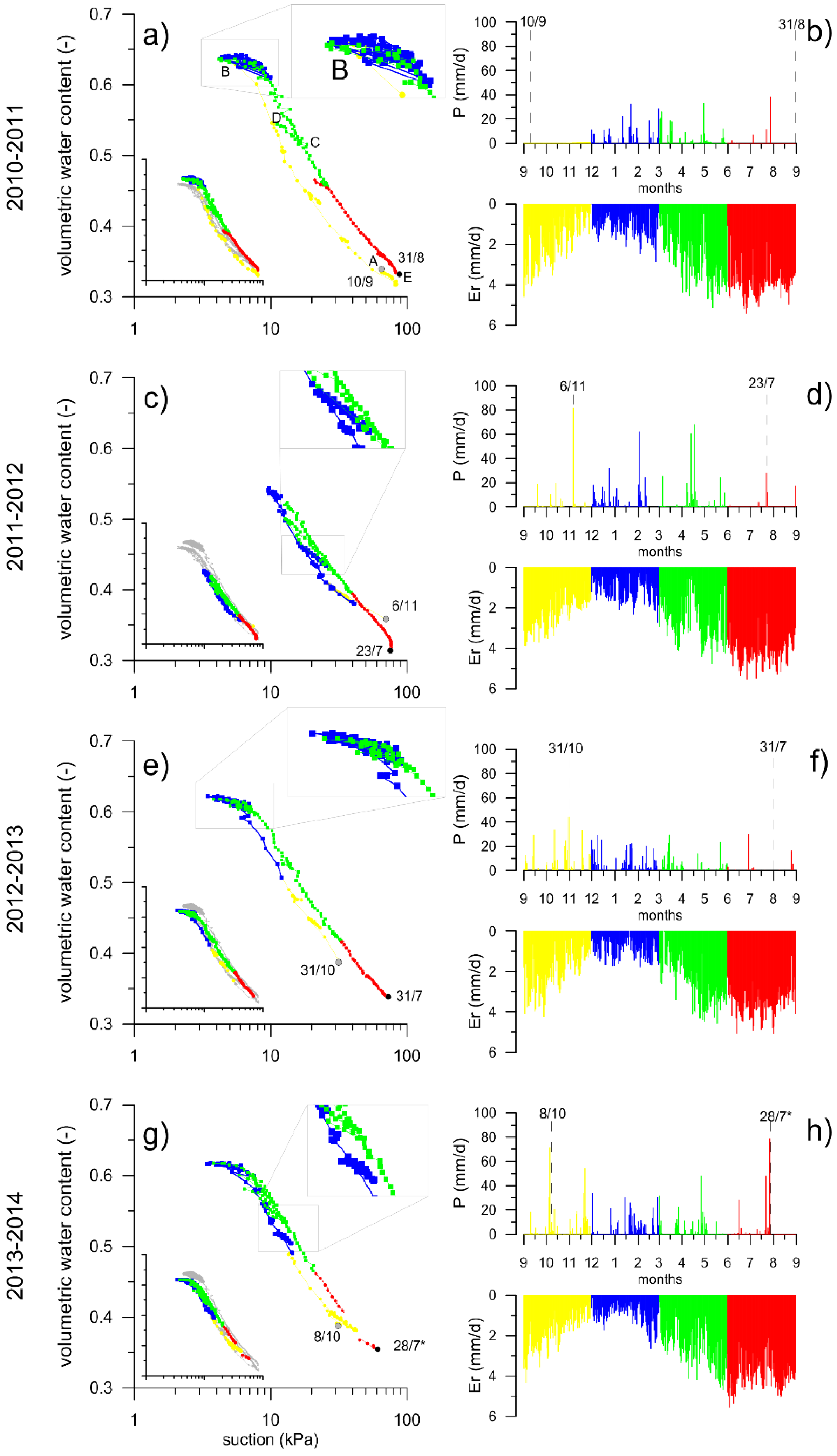
The results hereafter reported refer to an experimental phase lasting four hydrological years (from September 2010 to August 2014). In that time interval, the soil surface was maintained in a bare condition. SWCC data for the first and second hydrological years have been published by Rianna et al. [12]. For the sake of simplicity, the hydrological soil response analysis here only focuses on daily data obtained at a depth of 50 cm, which are summarized in Figure 4. The same figure reports the daily cumulated precipitation and the reference evaporative fluxes that have been estimated following the FAO–56 approach [32]. A hysteretic soil behavior clearly emerges from all readings which are here briefly analyzed.
In the 2010–2011 hydrological year (Figure 4a,b), the initial soil conditions (point A) were rather dry, characterized by a matric suction, s, of about 70 kPa and a volumetric water content, θ, of 0.35. However, the intense precipitation during the fall of 2010 moved the soil state from point A to B, along a wetting path leading s to 3–4 kPa and θ to 0.65. During winter the soil state fluctuated following different scanning paths which were always close to the saturated conditions. Due to frequent precipitation, the effects of drying, governed by a very low evaporative demand, and of wetting, never lead s beyond 15 kPa and θ below 0.6. In the early part of spring the soil maintained nearly saturated conditions, moving to different conditions only when the amount of precipitation significantly decreased while evaporation grew following the temperature rising. The consequent drying path (up to C) was completely different from the wetting path followed in the previous fall season. However, due to a heavy rainfall which lasted two days (30 April–1 May), the trend reversed at D, which represented a turning point, moving along a scanning path towards E. In the following dry period the drying path ran in the opposite direction along the same scanning curve, until reaching and following the previous main path. In this phase, the soil attained drier and drier states with only short reversions, during episodic rainfall events, along distinct scanning paths [33].
In the second hydrological year (2011–2012, Figure 4c,d), the atmospheric demand followed similar trends as in previous years, even though the cumulative rainfall was much lower. As a consequence, in winter the soil state was far from saturation, and matric suction was never less than 9 kPa or θ higher than 0.55. In this year, the attainment of suction values measurable with the tensiometer (i.e., below 80 kPa) presented a delay of about two months with respect to the previous year, caused by a daily rainfall (6 November) of 85 mm. Again, distinct paths characterized the principal wetting and drying phases. In two cases, reported in the zoom of Figure 4c, two scanning paths overlapped in the drying and wetting non-sequential phases.
During the third (2012–2013, Figure 4e,f) and fourth (2013–2014, Figure 4g,h) hydrological years, the cumulative rainfall attained values similar to the first year thus again, in winter, full soil saturation was almost attained. In this case, however, after running mostly along the same curve as in the first year, when approaching saturation the wetting path departs from it, moving to slightly lower θ values (0.62–0.63). This discrepancy was supposed to be an effect of some air entrapment that occurred under the effects of intermittent precipitation characterized by drier starting soil conditions. This interpretation was supported by the higher values measured during the fifth year [34] (not documented here) after a prolonged artificial wetting phase that was supposed to have removed air bubbles.
In conclusion, monitoring over four years clearly showed different drying and wetting paths, even though the most external ones could not be identified with certainty as the main drying or wetting curves. In particular, the slope of scanning paths appeared to be slightly affected by the initial state and by the wetting/drying direction.
3.2. Model Calibration and Validation
The PL model has been used to characterize the Monteforte Irpino ash used in the lysimeter experiments illustrated above [12]. The quantification of the seven parameters (θsd, θsw, θr, αd, αw, n, ks) has been obtained as follows. Four of them, i.e., θsd, θr, αd, n, were deduced by the experimental main drying curve obtained by imposing forced evaporation on an initially saturated soil sample in a ku-pF apparatus up to suction values of about 70 kPa. Dried soil cores were then placed in Richards’ plate up to 1000 kPa [10,35]. The last three parameters (θsw, αw, ks) were determined by calibration of the data provided by the lysimeter monitoring activity (§2.1) in the first year (Figure 4a). The parameters were validated through the data collected in the remaining three years (Figure 4b–d).
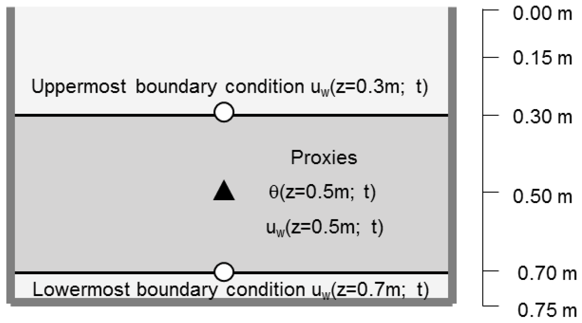
The parameter calibration was performed through an inverse analysis [36] carried out by the code Hydrus 1D [37]. The soil layer, with the middle at a depth of 50 cm (Figure 5) and thickness extending up and down to the nearby monitored depths (30 and 70 cm), was selected as a computational domain. In this way, the three suction monitored points (at 30, 50, and 70 cm) was used to model the transient flux governed, at the boundaries, by the total heads measured at depths of 30 and 70 cm, leading to the suction and volumetric water content readings made at a depth of 50 cm. The analysis required a value located on the main wetting or drying curve as a starting point; then, for every hydrological year, a subset of available observations was used for calibration and validation.
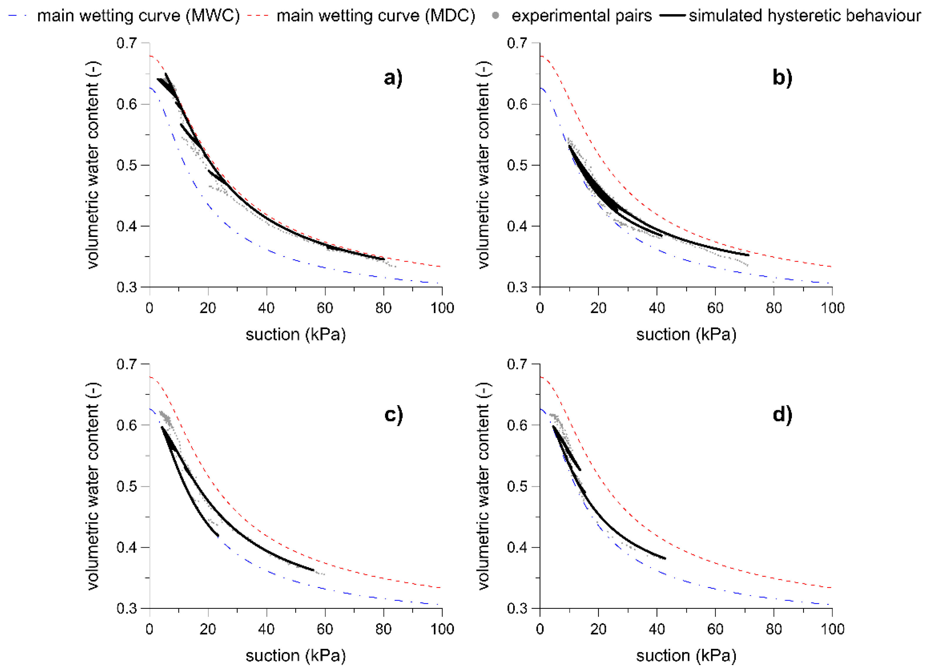
Figure 6a plots measured against predicted s–θ paths for the first year (calibration stage). The figure also reports the main drying and wetting curves obtained by laboratory data and calibration procedure, respectively. The predictions covering the three years of validation in blind configurations are shown in Figure 6b–d. The model indicates that most of the experimental paths follow scanning paths, either in wetting or in drying. The main drying and wetting curves have been only marginally ran; the former during the first year and the latter during the other years.
Table 1 lists the assessed hydraulic parameters for the MDC (main drying curve) and MWC (main wetting curve). Moreover, the parameters fitting the curve obtained by averaging the experimental results found by Rianna et al. [12] at a depth of 50 cm are reported (average curve, AC). Calibration returns a αw/αd ratio of 1.4, while literature indicates a value of 2 which appears to be suitable for many soils [35]. A hysteresis factor has also been analytically quantified through the effective hysteresis indicator proposed by Gebrenegus and Ghezzehei [38], which computes the maximum deviation in effective saturation between the two main curves. In Figure 7, the computed value is compared with the cloud of points provided by literature catalogues for a wide spectrum of materials, from fine-grained to coarse-grained soils [39,40,41]. Such a value falls around the middle of the cloud, indicating an intermediate behavior due to an intermediate grain size distribution (see Figure 2). Following the assessed value, the value of R computed according Equation (4) is about 16.5.
Finally, the saturated hydraulic conductivity resulting from calibration was 1 × 10⁻⁶ m/s, which is well higher than the value (ks = 3 × 10⁻⁷ m/s) obtained through laboratory tests [10], while it is equivalent to those carried out in the interpretation of monitoring results neglecting hysteresis [42].
3.3. Numerical Experiments on the Effects of Hydraulic Hysteresis in Landslide Triggering
3.3.1. Investigated Scenarios and Organization of Obtained Results
Some numerical experiments have been carried out to examine the effects of hydraulic hysteresis, in the wetting stage only, on the stability of virtual slopes subjected to precipitation. The analysis has been based on the following hypotheses:
- (1)
- (2)
- the lowermost boundary condition is modeled as a seepage surface, which behaves as an impervious boundary when suction remains higher than zero, and as a draining surface when it vanishes; this is the condition that has been recognized, through special targeted experiments, at the contact between ash and pumice layers [44];
- (3)
- two alternative hypotheses are adopted for the initial conditions: (A) constant piezometric head and (B) constant volumetric water content; the latter obviously results in an initial non-equilibrated suction profile;
- (4)
- a persistent 100 mm/day constant rainfall, slightly higher (~1.2 × 10⁻⁶ m/s) than the hydraulic conductivity of fully saturated soil, is imposed at the uppermost boundary condition; this is a realistic scenario in the considered geomorphological context, where such a daily rainfall intensity occurs every 2–3 years.
For sake of simplicity, the analysis was focused on the time required to reach zero matric suction, which occurred at a depth of 1.5 m (null suction time, NST). Such a condition, in fact, was found to mark the beginning of the failure process of several slopes in pyroclastic soils [1,6]. The NST was hence selected for a synthetic comparison of the influence of the wetting path on the soil hydrological response.
Four alternative hypotheses have been formulated about the (s, θ) relationship:
- -
- full hysteretic soil behavior (HB);
- -
- main drying curve (MDC);
- -
- main wetting curve (MWC);
- -
- the curve obtained by averaging the experimental results of Rianna et al. [12] at a depth of 50 cm (AC).
The analyses were carried out with the code Hydrus 1D, which can simulate the soil–atmosphere interaction by limiting potential fluxes (total precipitation and potential evaporation) based on the suction values computed at the uppermost surface [45].
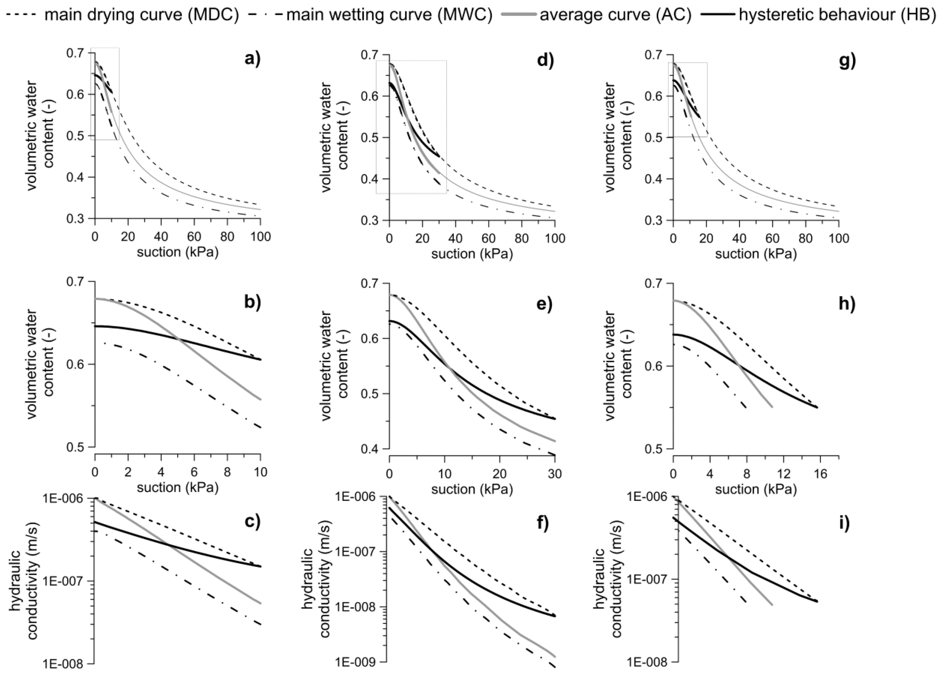
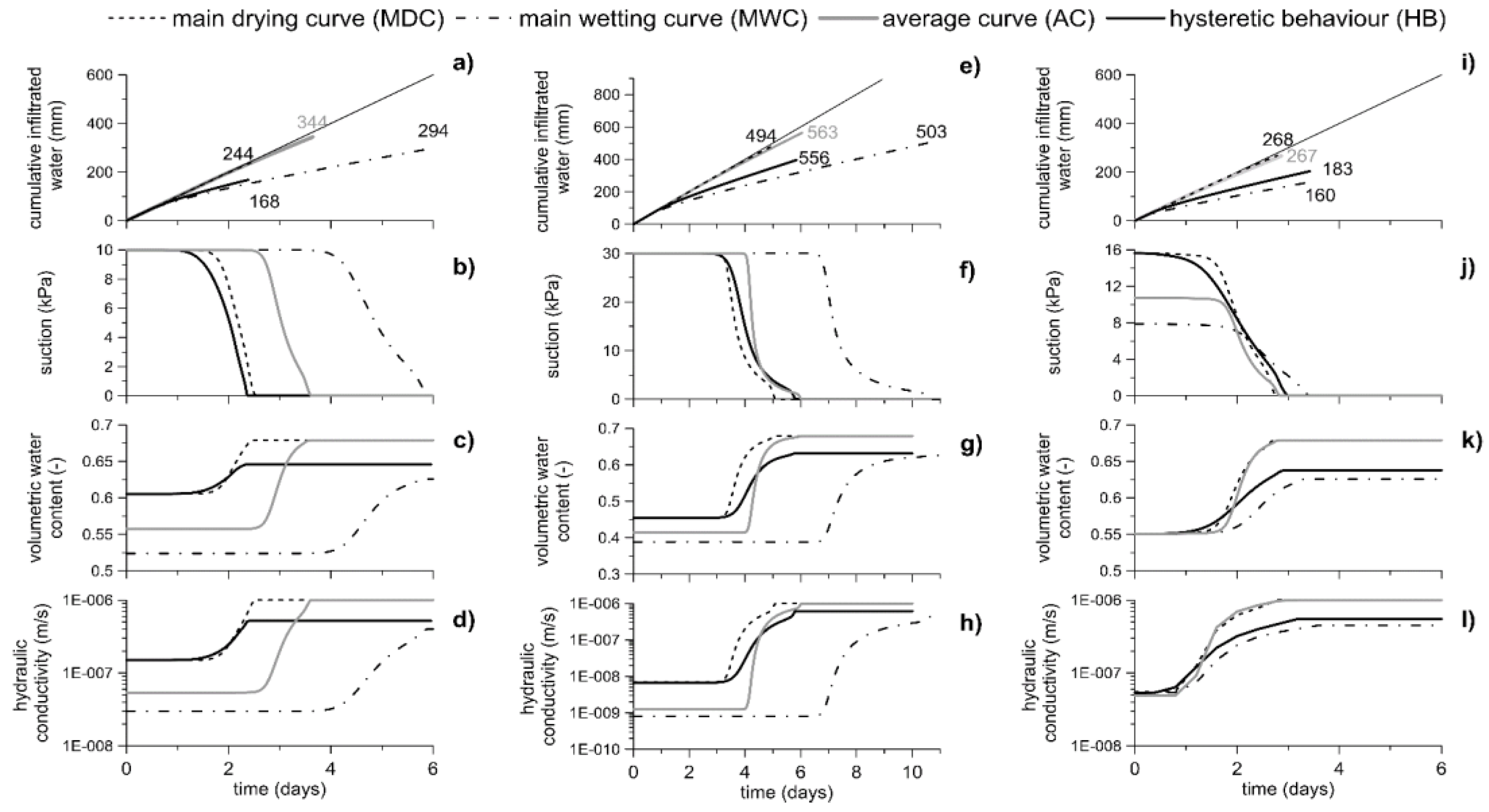
The main results of the analysis are reported in Figure 8, Figure 9 and Figure 10. The (s, θ) and (s, k) paths obtained at a depth of 1.5 m along any selected curve are compared in Figure 8: the first two columns concern case A and the different initial suction profiles characterized by 10 kPa and 30 kPa, respectively, at a depth of 1.5 m; the third column concerns case B (θ = 0.55). The time histories of the cumulative infiltrated water, suction, water content, and hydraulic conductivity are shown in Figure 9, respectively in the first, second, third, and fourth row. For the case A and the lowest initial suctions, Figure 10 compares the suction profiles computed at time intervals of 0.4 days.
3.3.2. Case A: Persistent Rainfall; Hydrostatic Initial Suction Profile
In case A, the initial water content, θ0, was univocally identified for all (s, θ) relationships, but only for the HB assumption, as this was not described by a single curve. For this last, θ0 has been conventionally established on the MDC (Figure 8a,b). The differences in soil behavior depending on the selected (s, θ) relationship are synthesized by the computed NST values.
Both HB and MDC yield a value of about 2.5 days (it is slightly shorter in the former case); moreover, AC yields a time length one-day longer (i.e., 3.5 days), while MWC leads to 6 days overall.
An interpretation of such results should obviously consider the two dominant factors which govern the process of suction change, i.e., the average hydraulic conductivity, kav, which is operative along the wetting path (as proxy, was considered the geometric mean), and the overall water content, Δθ, required to lead to zero suction. In the examined case (first column of Figure 8 and Figure 9), the values assumed by such parameters are as detailed in Table 2.
The combination of kav and Δθ clearly influences the soil response. In fact, the lower kav, the longer NST; conversely, the higher Δθ, the longer NST.
Limited to the assumption that the initial starting point for the HB relationship is located on the MDC (the initial condition depends on the past wetting/drying history), the considered example shows that the response provided by the more realistic HB is better approximated by MDC rather than, as often in practical applications, by AC or MWC.
Figure 9a reports the corresponding cumulated influx as 168 mm for HB (i.e., about 70% of the total rainwater fallen in the same period of 2.5 days) and 244 mm (i.e., practically the entire amount of rainfall) for MDC. Although associated with a similar increase in the volumetric water content (Figure 9c), the calculated influxes for AC and MWC are quite different, i.e., respectively 344 mm in about 3.5 days (about 100% of the total rainfall in the same time interval) and 294 mm in 6 days (about 50% of the total). The results obtained for higher suction values (30 kPa at 1.5 m, second column in Figure 8 and Figure 9) confirm the observed trends. Obviously, the higher the initial suction, the longer NST is due to a greater value of Δθ and to a lower hydraulic conductivity. Again, the rainfall duration to suction vanishing is shorter for HB and MDC, but the initial suction value can enhance the differences. However, under higher initial suction, the s–θ path potentially experienced along HB tends to progressively approach the one provided by MWC.
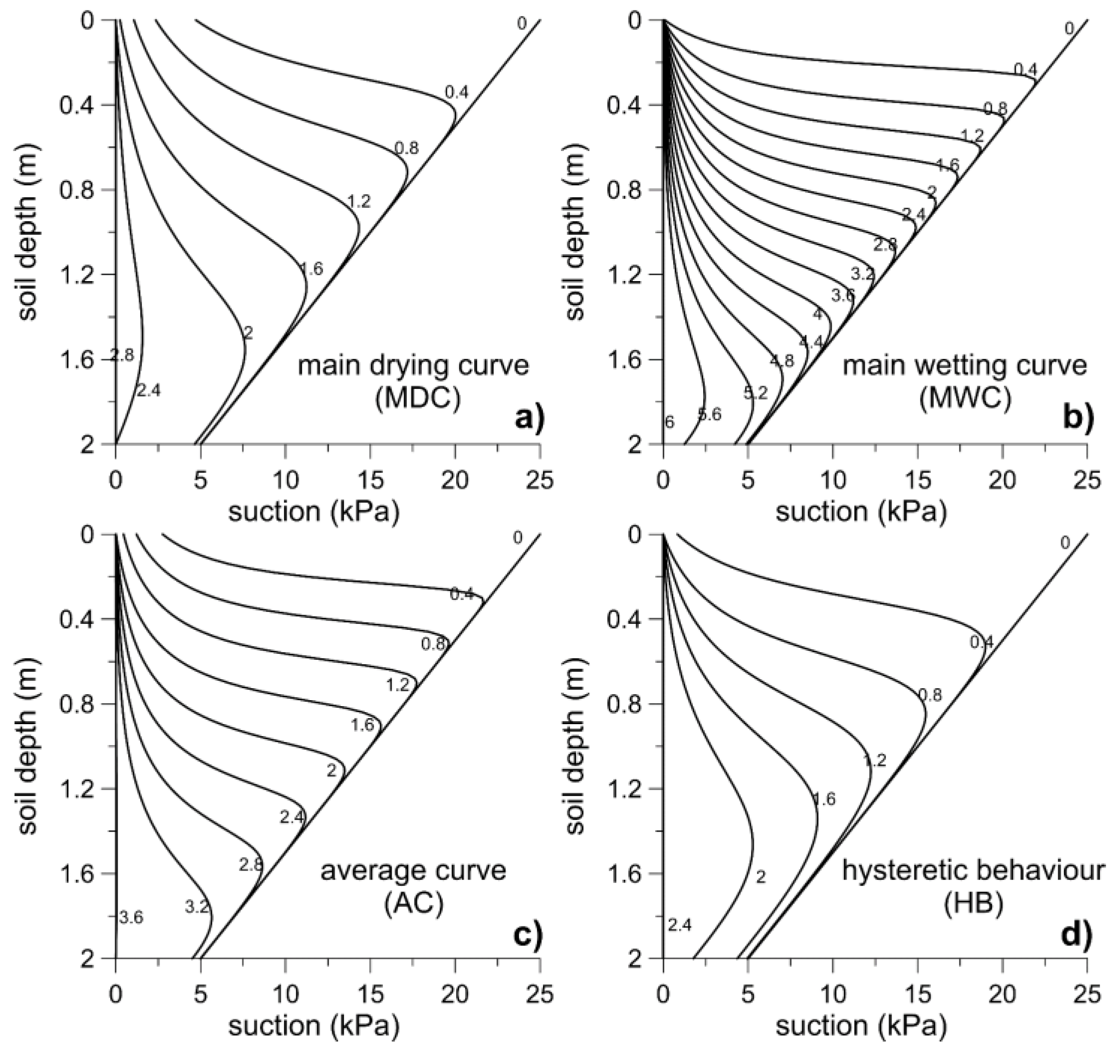
Figure 10 shows the suction profiles obtained at different times throughout the layer. If the soil behavior was governed by MWC or by AC, the wetting front would tend to deepen more slowly following a “Green–Ampt plunger type” evolution characterized by a sub-horizontal suction profile and a top to bottom front advance with marked frontal borders; the bottom of the layer would be reached after 5.2 and 3.2 days, respectively. Due to the higher hydraulic conductivity and the lower “stiffness” of the (s, θ) relationship, HB and MDC curves present less marked wet fronts. In this case, suction vanishing occurs in the final phases of the influx process through a shift of the suction profile which reaches the bottom faster, i.e., in something more than 2 days.
3.3.3. Case B: Persistent Rainfall; Uniform Initial Volumetric Water Content
The assumption of constant volumetric water content throughout the domain implies a similar initial hydraulic conductivity in all considered cases; moreover, if both MDC and MWC started and ended at zero suction, the Δθ values and the average operative hydraulic conductivities during the wetting processes would be the same as well. Therefore, similar time intervals NST would be predicted, with only small differences depending on the initial suction and thus on the potential infiltration. However, the fact that they did not end at zero suction, since the air entrapment effect was accounted for, implies that both Δθ and kav keep different values leading to different NSTs. In this case too, the initial conditions for HB were applied to MDC.
The analysis was carried out starting from a θ0 value of 0.55, which corresponded to a suction value of 8 kPa for MWC, 16 kPa for MDC (and HB), and 12 kPa for AC. The values of dominant factors and NSTs are reported in Table 3.
The analysis yielded quite similar NST values. The length of time was significantly different for MWC. The NST hierarchy was strictly regulated by kav, but the smaller variation in Δθ for the cases characterized by a lower hydraulic conductivity (MWC and HB) lead to smaller NST differences.
The rate of infiltrated water was significantly lower for MWC (160 mm in 3.5 days, on average 50% of fallen water) due to a lower hydraulic conductivity. For MDC and AC, the higher hydraulic conductivity favors water infiltration of most of the total precipitation.
4. Conclusions
Based on data provided by the monitoring of an instrumented layer of volcanic ash exposed to weather forcing over a period of four years, the hydraulic hysteretic behavior of such a soil was recognized and carefully investigated, allowing calibration and validation of the parameters featured in the Parker and Lenhard theoretical hysteretic model. Through some simple numerical experiments, the model was then used to investigate the role of hydraulic hysteresis upon wetting in the response of pyroclastic sloping covers to persistent rainfall. To this aim, different initial soil conditions in terms of suction and volumetric water content were considered. The data obtained was compared with those coming from more usual approaches that disregard the role of the hysteresis, resulting in a unique soil–water characteristic curve.
It has been shown that the time to suction vanishing due to continuous rainfall (which in some cases may correspond to the time to slope failure) may be much shorter than the value calculated using a unique curve, such as the main wetting curve or a curve averaging experimental data, which are usually adopted in applications. In the examined cases, the results are comparable with those provided by the main drying curve. The same findings come from cases characterized by the same initial matric suction or the same initial volumetric water content. As stressed above, it is worth noting, however, that the initial condition for soils exhibiting a marked hydraulic hysteresis may be variable, leading to different results. Such considerations should be kept in mind during the development of conceptual tools for landslide early warning systems.
Author Contributions
Methodology, all the authors; software analysis, A.R.; in situ investigation, L.P. (Luca Pagano), A.R., and G.R.; data curation, G.R.; Writing—Original Draft preparation, G.R. and A.R.; Writing—Review and Editing, L.C., L.P. (Luca Pagano), and L.P. (Luciano Picarelli); visualization, G.R. and A.R.; supervision, L.C., L.P. (Luca Pagano), and L.P. (Luciano Picarelli).
Funding
The APC was funded by “Progetto VALERE 2017—Open Access”.
Acknowledgments
L.C., L.Pa. and L.Pi. have partly developed this work within the framework of the PRIN 2015 project titled “Innovative Monitoring and Design Strategies for Sustainable Landslide Risk Mitigation”. They wish to thank the Ministero dell’Istruzione dell’Universitá e della Ricerca Scientifica (MIUR), which funded this project.
Conflicts of Interest
The authors declare no conflict of interest.
References
- Froude, M.J.; Petley, D.N. Global fatal landslide occurrence from 2004 to 2016. Nat. Hazards Earth Syst. Sci. 2018, 18, 2161–2181. [Google Scholar] [CrossRef]
- Pagano, L.; Picarelli, L.; Rianna, G.; Urciuoli, G. A simple numerical procedure for timely prediction of precipitation–induced landslides in unsaturated pyroclastic soils. Landslides 2010, 7, 273–289. [Google Scholar] [CrossRef]
- Rianna, G.; Pagano, L.; Urciuoli, G. Rainfall patterns triggering shallow flowslides in pyroclastic soils. Eng. Geol. 2014, 174, 22–35. [Google Scholar] [CrossRef]
- Iverson, R.M. Landslide triggering by rain infiltration. Water Resour. Res. 2000, 36, 1897–1910. [Google Scholar] [CrossRef] [Green Version]
- Cascini, L.; Guida, D.; Romanzi, G.; Nocera, N.; Sorbino, G. A preliminary model for the landslides of May 1998 in Campania Region. In Proceedings of the International Symposium on The Geotechnics of Hard Soils—Soft Rocks, Naples, Italy, 12–14 October 1998; Evangelista, A., Picarelli, L., Eds.; 1998; Volume 3, pp. 1623–1652. [Google Scholar]
- Olivares, L.; Picarelli, L. Shallow flowslides triggered by intense rainfalls on natural slopes covered by loose unsaturated pyroclastic soils. Geotechnique 2003, 532, 283–287. [Google Scholar] [CrossRef]
- Nocentini, M.; Tofani, V.; Gigli, G.; Fidolini, F.; Casagli, N. Modeling debris flows in volcanic terrains for hazard mapping: The case study of Ischia Island (Italy). Landslides 2015, 12, 831–846. [Google Scholar] [CrossRef]
- Picarelli, L.; Evangelista, A.; Rolandi, G.; Paone, A.; Nicotera, M.V.; Olivares, L.; Scotto di Santolo, A.; Lampitiello, S.; Rolandi, M. Mechanical properties of pyroclastic soils in Campania Region. In Proceedings of the 2nd International Workshop on Characterisation and Engineering Properties of Natural Soils, Singapore, 29 November–1 December 2006; Tan, T.S., Phoon, K.K., Height, D.W., Leroueil, S., Eds.; Taylor & Francis Group: London, UK, 2006; Volume 4, pp. 2331–2384. [Google Scholar]
- Nicotera, M.V.; Papa, R.; Urciuoli, G. An experimental technique for determining the hydraulic properties of unsaturated pyroclastic soils. Geotech. Test. J. 2010, 33, 263–285. [Google Scholar]
- Pirone, M.; Papa, R.; Nicotera, M.V.; Urciuoli, G. In situ monitoring of the groundwater field in an unsaturated pyroclastic slope for slope stability evaluation. Landslides 2015, 12, 259–276. [Google Scholar] [CrossRef]
- Damiano, E.; Olivares, L.; Picarelli, L. Steep–slope monitoring in unsaturated pyroclastic soils. Eng. Geol. 2012, 137, 1–12. [Google Scholar] [CrossRef]
- Rianna, G.; Pagano, L.; Urciuoli, G. Investigation of soil–atmosphere interaction in pyroclastic soils. J. Hydrol. 2014, 510, 480–492. [Google Scholar] [CrossRef]
- Comegna, L.; Damiano, E.; Greco, R.; Guida, A.; Olivares, L.; Picarelli, L. Field hydrological monitoring of a sloping shallow pyroclastic deposit. Can. Geotech. J. 2016, 53, 1125–1137. [Google Scholar] [CrossRef] [Green Version]
- Olivares, L.; Picarelli, L. Modelling of flowslides behaviour for risk mitigation. In Proceedings of the 6th International Conference on Physical Modelling in Geotechnics, Hong Kong, China, 4–6 August 2006; Taylor & Francis: London, UK, 2006; Volume 1, pp. 99–112. [Google Scholar]
- Cascini, L.; Cuomo, S.; Pastor, M.; Sorbino, G.; Piciullo, L. SPH run–out modelling of channelized landslides of the flow type. Geomorphology 2014, 214, 502–513. [Google Scholar] [CrossRef]
- Pirone, M.; Papa, R.; Nicotera, M.V.; Urciuoli, G. Evaluation of the Hydraulic Hysteresis of Unsaturated Pyroclastic Soils by in Situ Measurements. Proced. Earth Planet. Sci. 2014, 9, 163–170. [Google Scholar] [CrossRef] [Green Version]
- Comegna, L.; Damiano, E.; Greco, R.; Guida, A.; Olivares, L.; Picarelli, L. Investigation on the hydraulic hysteresis of a pyroclastic deposit. In Proceedings of the International Workshop on Volcanic Rocks and Soils, Ischia, Italy, 24–25 September 2015; pp. 161–162. [Google Scholar]
- Basile, A.; Ciollaro, G.; Coppola, A. Hysteresis in soil water characteristics as a key to interpreting comparisons of laboratory and field measured hydraulic properties. Water Resour. Res. 2003, 39, 1355. [Google Scholar] [CrossRef]
- Comegna, L.; Rianna, G.; Lee, S.; Picarelli, L. Influence of the wetting path on the mechanical response of shallow unsaturated sloping covers. Comput. Geotech. 2016, 73, 164–169. [Google Scholar] [CrossRef]
- Richards, L.A. Capillary conduction of liquids through porous mediums. Physics 1931, 1, 318–333. [Google Scholar] [CrossRef]
- Van Genuchten, M.T. A closed form equation for predicting the hydraulic conductivity. Soil Sci. Soc. Am. J. 1980, 44, 892–898. [Google Scholar] [CrossRef]
- Mualem, Y. A new model for predicting the hydraulic conductivity of unsaturated porous media. Water Resour. Res. 1976, 12, 513–522. [Google Scholar] [CrossRef]
- Viaene, P.; Vereecken, H.; Diels, J.; Feyen, J. A statistical analysis of six hysteresis models for the moisture retention characteristic. Soil Sci. 1994, 157, 345–355. [Google Scholar] [CrossRef]
- Pham, H.Q.; Fredlund, D.G.; Barbour, S.L. A study of hysteresis models for soil-water characteristic curves. Can. Geotech. J. 2005, 42, 1548–1568. [Google Scholar] [CrossRef]
- Bashir, R. Quantification of Surfactant Induced Unsaturated Flow in the Vadose Zone. Ph.D. Thesis, McMaster University, Hamilton, ON, Canada, 2007. [Google Scholar]
- Parker, J.C.; Lenhard, R.J. A model for hysteretic constitutive relations governing multiphase flow: 1. Saturation–pressure relations. Water Resour. Res. 1987, 23, 2187–2196. [Google Scholar] [CrossRef]
- Scott, P.; Farquhar, G.; Kouwen, N. Hysteretic effects on net infiltration. In Advances in Infiltration; ASCE: Reston, VA, USA, 1983; pp. 163–170. [Google Scholar]
- Kool, J.B.; Parker, J.C. Development and evaluation of closed–form expressions for hysteretic soil hydraulic properties. Water Resour. Res. 1987, 23, 105–114. [Google Scholar] [CrossRef]
- Werner, A.D.; Lockington, D.A. Artificial pumping errors in the Kool– Parker scaling model of soil moisture hysteresis. J. Hydrol. 2006, 325, 118–133. [Google Scholar] [CrossRef]
- Land, C.S. Calculation of Imbibition Relative Permeability for Two– and Three–Phase Flow from Rock Properties. Soc. Pet. Eng. J. 1968, 8, 149–156. [Google Scholar] [CrossRef]
- Lenhard, R.J.; Parker, J.C. A Model for Hysteretic Constitutive Relations Governing Multiphase Flow 2. Water Resour. Res. 1987, 23, 2197–2206. [Google Scholar] [CrossRef]
- Allen, R.G.; Pereira, L.S.; Raes, D.; Smith, M. Crop Evapotranspiration: Guidelines for Computing Crop Requirements. Irrigation and Drainage Paper No. 56; FAO: Rome, Italy, 1998. [Google Scholar]
- Rianna, G.; Reder, A.; Pagano, L. Estimating actual and potential bare soil evaporation from silty pyroclastic soils: Towards improved landslide prediction. J. Hydrol. 2018, 562, 193–209. [Google Scholar] [CrossRef]
- Pagano, L.; Reder, A.; Rianna, G. Effects of vegetation on hydrological response of silty volcanic covers. Can. Geotech. J. 2018. [Google Scholar] [CrossRef]
- Fredlund, D.G.; Rahardjo, H.; Fredlund, M.D. Unsaturated Soil Mechanics in Engineering Practice; John Wiley & Sons, Inc.: Hoboken, NJ, USA, 2012. [Google Scholar]
- Hopmans, J.W.; Šimůnek, J.W.; Romano, N.; Durner, W. Inverse Methods. In Methods of Soil Analysis—Part 4—Physical Methods; Dane, J.H., Topp, G.C., Eds.; SSSA Book Ser. 5; SSSA: Madison, WI, USA, 2014; pp. 963–1008. [Google Scholar]
- Šimunek, J.; Šejna, M.; Saito, H.; Sakai, M.; van Genuchten, M.T. The Hydrus–1D Software Package for Simulating the Movement of Water, Heat, and Multiple Solutes in Variably Saturated Media. Version 4.17. Hydrus Software Series 3; Department of Environmental Sciences, University of California Riverside: Riverside, CA, USA, 2013. [Google Scholar]
- Likos, W.J.; Lu, N.; Godt, J.W. Hysteresis and Uncertainty in Soil Water–Retention Curve Parameters. J. Geotech. Geoenv. Eng. 2014, 140, 04013050. [Google Scholar] [CrossRef]
- Gebrenegus, T.; Ghezzehei, T.A. An index for degree of hysteresis in water retention. Soil Sci. Soc. Am. J. 2011, 75, 2122–2127. [Google Scholar] [CrossRef]
- Yang, C.; Sheng, D.; Carter, J.P. Effect of Hydraulic Hysteresis on Seepage Analysis for Unsaturated Soils. Comput. Geotech. 2012, 41, 36–56. [Google Scholar] [CrossRef]
- Huang, H.C.; Tan, Y.C.; Liu, C.W.; Chen, C.H. A novel hysteresis model in unsaturated soil. Hydrol. Process. 2005, 19, 1653–1665. [Google Scholar] [CrossRef]
- Reder, A.; Rianna, G.; Pagano, L. Physically based approaches incorporating evaporation for early warning predictions of rainfall–induced landslides. Nat. Hazards Earth Syst. Sci. 2018, 18, 613–631. [Google Scholar] [CrossRef]
- Di Crescenzo, G.; Santo, A. Debris slides–rapid earth flows in the carbonate massifs of the Campania region (Southern Italy): Morphological and morphometric data for evaluating triggering susceptibility. Geomorphol. 2005, 66, 255–276. [Google Scholar] [CrossRef]
- Reder, A.; Pagano, L.; Picarelli, L.; Rianna, G. The role of the lowermost boundary conditions in the hydrological response of shallow sloping covers. Landslides 2017, 14, 861–873. [Google Scholar] [CrossRef]
- Feddes, R.A.; Bresler, E.; Neuman, S.P. Field test of a modified numerical model for water uptake by root systems. Water Resour. Res. 1974, 10, 1199–1206. [Google Scholar] [CrossRef]
Figure 1.
Physical model sketch with instrumentation.

Figure 2.
Grain size distribution of the investigated soil.

Figure 3.
(a) Scanning path scenarios for the hysteretic PL model; (b) effect of air entrapment.

Figure 4.
First column (a,c,e,g): matric suction–volumetric water content paths observed at depth of 50 cm over four hydrological years: yellow = fall–SON (September-October-November), blue = winter–DJF (December-January-February), green = spring–MAM (March-April-May), black, red = summer–JJA (June-July-August); in the box, readings made in other years and zooms of key paths are also reported. Second column (b,d,f,h): daily precipitation and reference evaporation assessed through the FAO approach: yellow = fall–SON, blue = winter–DJF, green = spring–MAM, red = summer–JJA.

Figure 5.
Soil domain investigated for calibration and validation of the soil parameters.

Figure 6.
Observed (grey dots) and simulated (black line) matric suction–volumetric water content paths for the four hydrological years: 2010–2011 (a), 2011–2012 (b), 2012–2013 (c), and 2013–2014 (d). Main drying curve: red dashed line; main wetting curve: blue dot-line hatching.
Figure 6.
Observed (grey dots) and simulated (black line) matric suction–volumetric water content paths for the four hydrological years: 2010–2011 (a), 2011–2012 (b), 2012–2013 (c), and 2013–2014 (d). Main drying curve: red dashed line; main wetting curve: blue dot-line hatching.

Figure 7.
Hysteresis factor as function of parameter n of the van Genuchten model. Hollow circles: data provided by literature datasets, filled circles: values calculated in the present investigation.
Figure 7.
Hysteresis factor as function of parameter n of the van Genuchten model. Hollow circles: data provided by literature datasets, filled circles: values calculated in the present investigation.

Figure 8.
First and second row: volumetric water content–suction (s–θ) plane; third row: suction–hydraulic conductivity (s–k) plane. Black dashed line: main drying curve; dot-line hatching: main wetting curve; continuous grey line: average curve; black line: scanning paths; thick lines: paths followed in the numerical experiments. First column: hydrostatic initial condition with 10 kPa at 1.5 m. Second column: hydrostatic initial condition with 30 kPa at 1.5 m. Third column: constant volumetric water content (0.55).

Figure 9.
Results of analyses conducted up to suction vanishing at a depth of 1.5 m. First row: cumulative infiltrated water (dotted black line: cumulated rainfall). Second row: suction evolution. Third row: volumetric water content evolution. Fourth row: hydraulic conductivity evolution. First column: hydrostatic initial condition with 10 kPa at 1.5 m. Second column: hydrostatic initial condition with 30 kPa at 1.5 m. Third column: constant volumetric water content (0.55). Hydraulic behavior are identified as in Figure 8.

Figure 10.
Calculated matric suction profiles through the soil hydrostatic initial conditions. Figures refer to different time steps (day). (a) MDC; (b) MWC; (c) AC; (d) HB.
Figure 10.
Calculated matric suction profiles through the soil hydrostatic initial conditions. Figures refer to different time steps (day). (a) MDC; (b) MWC; (c) AC; (d) HB.


Table 1.
Parameters regulating the hydraulic behavior of investigated soil under the different adopted characterizations: MDC (main drying curve), MWC (main wetting curve), and AC (average curve).
Table 1.
Parameters regulating the hydraulic behavior of investigated soil under the different adopted characterizations: MDC (main drying curve), MWC (main wetting curve), and AC (average curve).
| Hydraulic Characterization | θs | θr | α (1/kPa) | N | ks (m/s) |
|---|---|---|---|---|---|
| MDC | 0.679 | 0.260 | 0.07 | 1.9 | 1.00 × 10⁻⁶ |
| MWC | 0.626 | 0.260 | 0.10 | 1.9 | 3.00 × 10⁻⁷ |
| AC | 0.679 | 0.288 | 0.11 | 1.9 | 1.00 × 10⁻⁶ |
Table 2.
Dominant factors (kav = average hydraulic conductivity; Δθ = overall water content) in case A: HB (hysteretic behavior), MDC (main drying curve), MWC (main wetting curve), and AC (average curve).
Table 2.
Dominant factors (kav = average hydraulic conductivity; Δθ = overall water content) in case A: HB (hysteretic behavior), MDC (main drying curve), MWC (main wetting curve), and AC (average curve).
| Hydraulic Characterization | Δθ | kav (m/s) |
|---|---|---|
| HB | 0.04 | 3.90 × 10⁻⁷ |
| MDC | 0.07 | 2.25 × 10⁻⁷ |
| MWC | 0.11 | 1.00 × 10⁻⁷ |
| AC | 0.12 | 2.39 × 10⁻⁷ |
Table 3.
Dominant factors (kav = average hydraulic conductivity; Δθ = overall water content) and NST (null suction time) in case B: HB (hysteretic behavior), MDC (main drying curve), MWC (main wetting curve), and AC (average curve).
Table 3.
Dominant factors (kav = average hydraulic conductivity; Δθ = overall water content) and NST (null suction time) in case B: HB (hysteretic behavior), MDC (main drying curve), MWC (main wetting curve), and AC (average curve).
| Hydraulic Characterization | Δθ | kav (m/s) | NST (Days) |
|---|---|---|---|
| HB | 0.09 | 1.72 × 10⁻⁷ | 3.0 |
| MDC | 0.13 | 2.34 × 10⁻⁷ | 2.8 |
| MWC | 0.08 | 1.55 × 10⁻⁷ | 3.5 |
| AC | 0.13 | 2.22 × 10⁻⁷ | 2.9 |
© 2019 by the authors. Licensee MDPI, Basel, Switzerland. This article is an open access article distributed under the terms and conditions of the Creative Commons Attribution (CC BY) license (http://creativecommons.org/licenses/by/4.0/).
Share and Cite
MDPI and ACS Style
Rianna, G.; Comegna, L.; Pagano, L.; Picarelli, L.; Reder, A. The Role of Hydraulic Hysteresis on the Hydrological Response of Pyroclastic Silty Covers. Water 2019, 11, 628. https://doi.org/10.3390/w11030628
AMA Style
Rianna G, Comegna L, Pagano L, Picarelli L, Reder A. The Role of Hydraulic Hysteresis on the Hydrological Response of Pyroclastic Silty Covers. Water. 2019; 11(3):628. https://doi.org/10.3390/w11030628
Chicago/Turabian StyleRianna, Guido, Luca Comegna, Luca Pagano, Luciano Picarelli, and Alfredo Reder. 2019. "The Role of Hydraulic Hysteresis on the Hydrological Response of Pyroclastic Silty Covers" Water 11, no. 3: 628. https://doi.org/10.3390/w11030628
Note that from the first issue of 2016, this journal uses article numbers instead of page numbers. See further details here.