Uncertainty in Irrigation Technology: Insights from a CGE Approach


Department of Economic Analysis, University of Zaragoza, Zaragoza, Spain and AgriFood Institute of Aragon (IA2), 50005 Zaragoza, Spain
*
Author to whom correspondence should be addressed.
Water 2019, 11(3), 617; https://doi.org/10.3390/w11030617
Submission received: 21 October 2018
/
Revised: 13 February 2019
/
Accepted: 15 March 2019
/
Published: 25 March 2019
(This article belongs to the Special Issue Water Resources Management and Policy Development: International Security and Economic Relations)
Abstract
:The benefits of technological improvement are uncertain. The timing of the introduction and take-up of new technologies is difficult to estimate. Technological improvements play a decisive role in water policy. In the context of water policy design, we evaluate the implications of uncertainty in the gradual process of enhancements to the efficiency of irrigation water use, for a better understanding of the extent to which these improvements could mitigate the output losses derived from water constraints. To accomplish this, we address simultaneous sensitivity analyses within a dynamic Computable General Equilibrium (CGE) model to analyze different uncertainty scenarios. Our results show that the date on which advanced technology becomes available and enters general use is quite significant. The greater and faster the improvements in irrigation technologies, the better.
JEL Classification:
C68; D80; O30; Q251. Introduction
The main purpose of the present work is to evaluate the implications of uncertainty in the gradual process of enhancements to the efficiency of irrigation water use, derived from a policy of modernization. This allows a better understanding both of the extent to which these improvements can mitigate the output losses derived from water constraints and the uncertainty effects in this mitigation related, for instance, to the timing of the introduction and take-up of new technologies. The possibility that such gains will never reach a level of advanced efficiency is also considered in line with recent studies that have shown that technology spillovers could not be observed, in spite of investment and the capacity to absorb innovations [1].
A number of studies have highlighted the importance of dealing with uncertainty in both technological change and climate change ([2,3,4,5]). Uncertainty is a key issue for the design of climate change policy. The timing of the introduction of new technologies and the take-up of those technologies is difficult to estimate and is, therefore, uncertain. A decisive role in water policy is played by technological improvements. Prior studies have seen both risk and uncertainty in, for example, the implementation process of agricultural technology innovation for farmers ([6,7]). Moreover, that uncertainty also extends to the availability of water resources. A review of papers dealing with uncertainty in different areas, such as climate damage, technological change, and emissions policies, can be found in [4], which discusses the various conclusions of a range of studies and highlights the different lines of research. More recently, Berck, P. et.al [8] presented a framework to make better decisions when facing different sources of threats, differentiating uncertainty as endogenous when it is created by human action or exogenous if it is created by nature, and address both risks at the same time. In this context, this work mainly addresses uncertainty as internal risk based on uncertainty in the gradual process of enhancements to the efficiency of irrigation water use by farmers through an irrigation modernization process.
To this end, our work stems from a prior study of technological change in irrigated agriculture, taking the largest irrigation scheme in the Ebro River Basin (Spain) as a case study (see [9]). The region is semi-arid, suffers from irregular and significant water shortages, and is in the midst of a modernization process of irrigated land to switch from flood irrigation to sprinkler and drip irrigation systems. The water supply in the Ebro River Basin is irregular and there are serious doubts about its future trends. However, some studies have recently identified a cyclical and decreasing evolution in water flows that lets us assume a forecast framework of water supply based on the observed evolution [10].
For the purpose of this paper, we use a recursive dynamic computable general equilibrium (CGE) model that includes elements that allow us to consider different alternatives for its evolution simultaneously and involve all variables of the general equilibrium model (prices, outputs, taxes, demands,…) although assuming perfect foresight of water supply into the distant future for each alternative. CGE models are empirical versions of a Walrasian model, formalized by [11] and based on a set of numerical equations that capture the characteristics and general functioning of an economy. These models can measure both direct and indirect effects of alternative economic policies, as well as changes in the behaviour of economic agents. CGE models let us take into account the global impact in all sectors and agents after a shock in a specific sector, including price and rebound effects of technological improvements, which cannot be analyzed with partial equilibrium models.
CGE models have been widely used in recent years to address the impacts of climate change and greenhouse gas (GHG) emissions ([12,13,14,15,16,17]) and also to address the management of water resources ([9,18,19,20,21,22,23,24]). As these models consider the various linkages between economic sectors, they are particularly useful for the evaluation of water-pricing policies, due to the ability of these models to calculate both equilibrium prices and quantities [25]. Such models have become a standard tool in the quantitative analysis of policy intervention in many domains, including fiscal policy, trade policy, and environmental policy [26]. Additionally, these models have been extended to consider risk and uncertainty. Goodman, D.J. et. al [27] presented a review of computable general equilibrium models that consider risk and quantify the monetary value of risk by incorporating uncertainty by formulating different paths in a CGE model. Harrison, G.W. et. al [28] use stochastic structures to analyze the optimal policy mix between taxing emissions and subsidizing technologies in Research and Development programs, taking into account the date on which the advanced technology became available. The stochastic programming includes a set of possible states that is included in each variable of the model, and each possible state involves a different probability. They find that policy recommendations are different when uncertainty in technical change is modeled than when it is not. Moreover, as [4] point out, these results demonstrate that the implications of uncertainty cannot always be only inferred from the standard sensitivity analysis of the model parameters. Heal, G. et. al [29] show how uncertainty about the 2020–2050 emissions targets may affect CO2 and energy prices, as well as technological choices in the energy sector. To do this, they develop stochastic policy scenarios within a CGE framework to analyze CO2 prices.
Therefore, the main contribution of this work is to use a recursive dynamic CGE model, in order to address the effects of uncertainty in the gradual process of enhancements to the efficiency of irrigation water, focusing on the uncertainty in the timing of the introduction and take-up of new technologies. As far as we are aware, very few studies have so far incorporated uncertainty in CGE models in this area (see [27,28], among others). Pervasive uncertainty, the likely revision of policies over time, and unexpected changes in technology, suggest the need for a recursive-dynamic solution in the CGE analysis, as [2,30] conclude. Solving a complex CGE model was, until recently, difficult due to our limited computational resources, but the use of such complex models has become possible following advances in mathematical programming and software, which have facilitated the design of structures rooted in economic reality to reflect modeller objectives and the common sense of policy-making, in order to arrive at viable conclusions and to assess the implications of a wide spectrum of possible results.
2. The Extended Model
2.1. Outline of the Model
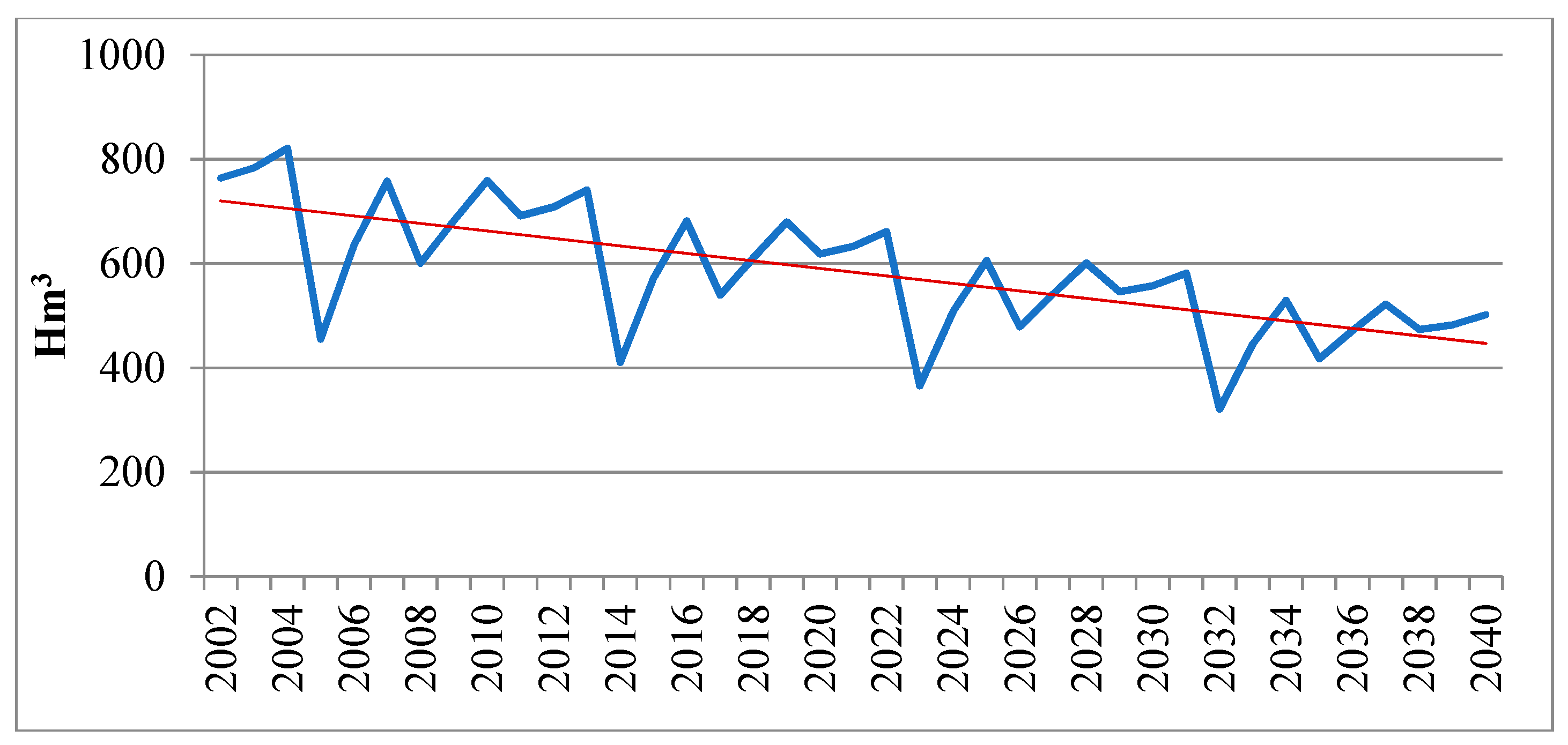
Our model represents the economy of Huesca province. This province is selected because it contains the largest irrigation scheme in Spain, the Upper Aragon Irrigation Scheme (CGRAA is the Spanish acronym), that is one of the most ambitious projects of its kind in the country [31]. The CGRAA irrigates more than 125,000 hectares of land and comprises 58 irrigation sub-schemes, supplying water to a number of municipalities, as well as 10 industrial estates. However, this irrigation scheme is facing a downward trend in water supply (see [11,32]) that involves pressure on the water supply available for irrigation. The trend followed by water for industrial uses is very different, even increasing in drought years. In light of this, we consider only irrigation water uses. However, industrial water represents only a small share of total use (less than 1%) and its exclusion does not significantly change our results. See actual data of the water supply in Figure 4 in Section 3.
Our database of the Huesca province economy includes 18 sectors, where farming is disaggregated into irrigated agriculture, rainfed agriculture and livestock farming. Additionally, irrigated agriculture is broken down into four sectors: cereals and legumes; industrial crops; fruit and vegetables; olives and vineyards. We use the structure of the model described in detail in [9], and we extend the model in this work to include different weighted alternatives simultaneously, as is shown in the following subsection.
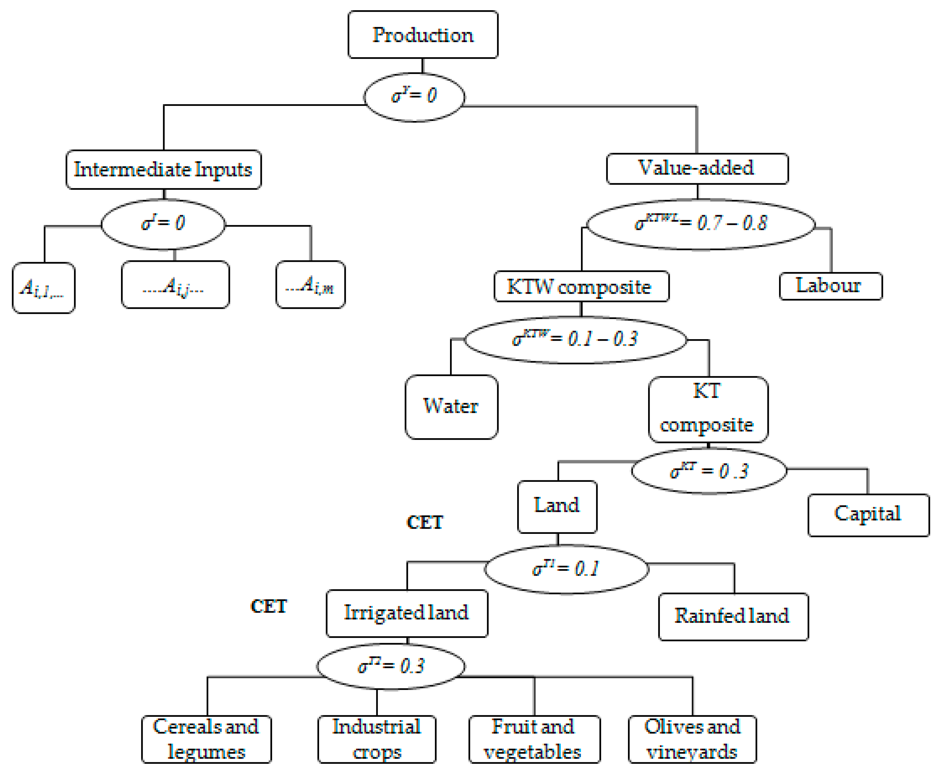
Figure 1 shows the structure of technology used in the model for the irrigated agriculture sectors. Producer behaviour includes a nested constant elasticity of substitution (CES) production function in four-stages. These functions are widely used in CGE modelling due to their flexibility of substitution. Total production is obtained through a combination of intermediate inputs and value-added following a Leontief function. Then, the value-added separates labor from the aggregate of capital, land and water called KTW composite. This KTW bundle combines a capital–land (KT) bundle with water through an elasticity of substitution whose values vary for each crop because water and land are expected to be reallocated in the case of a declining water supply. The selection of the elasticity parameters is presented in Table S1 of the Supplementary Information. The inclusion of the nested constant CES improves the flexibility of the model instead of considering land and water as fixed coefficients (as in [33]), in line with [18,34].
Additionally, the use of land is implemented using a Constant Elasticity of Transformation (CET) function (see [35,36,37]). This adaptation allows us to allocate land first between irrigated and rainfed land, and at a second level, within all irrigated crops. As the rainfed agricultural sector does not use water, labor is combined with a capital–land bundle. The rest of the sectors (industry and services) combine water with capital, as they do not use the land factor.
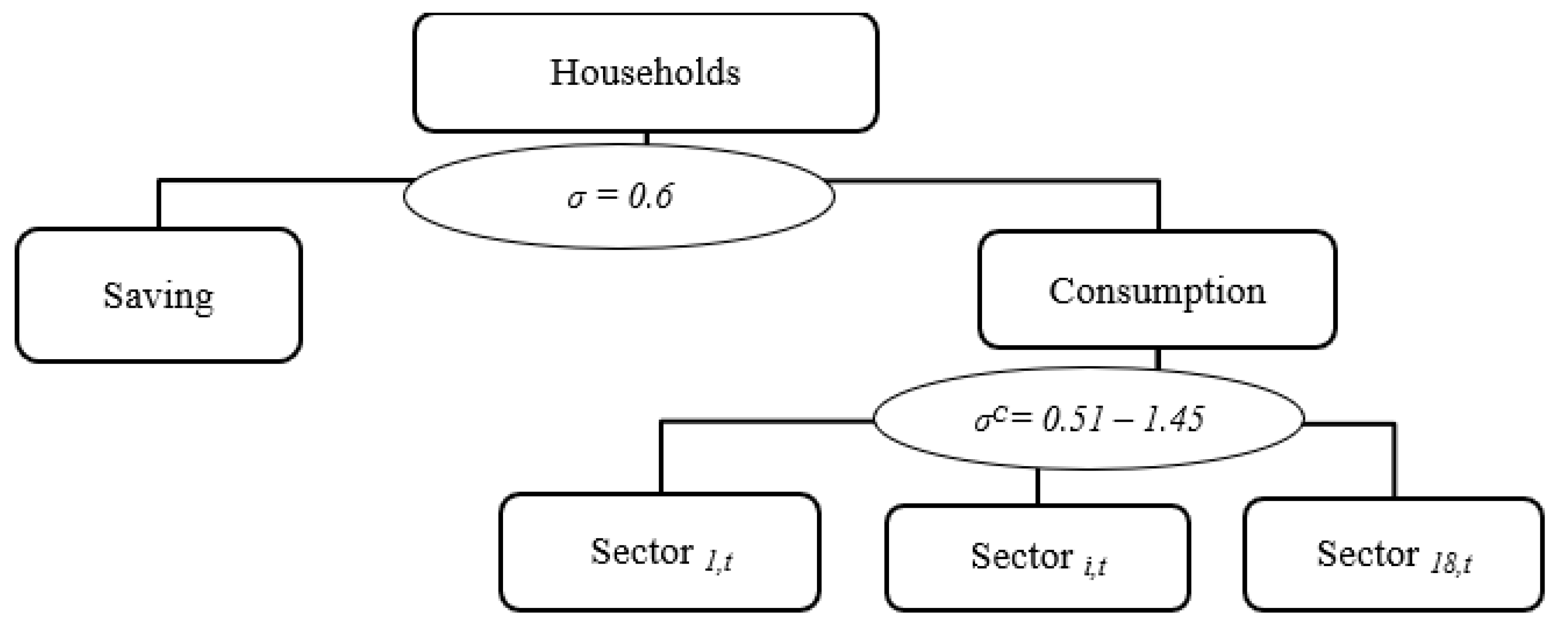
Regarding trade, a CET function and the Armington approach [38] are used between domestic and foreign demands. The consumption structure is also established using a CES utility function (see Figure 2).
Regarding closure rules, we assume lump-sum transfers between the Government and the agents, to ensure the same budget balance as in the base year. We include an additional agent (Farmer) in the model to collect the mark-up on the cost of water and receipts are earmarked to pay modernization costs, in a similar way to a Water Board and the CGRAA. Labor and capital factors are considered perfectly mobile across sectors. Water supply is assumed to be exogenous, as we can see in our scenarios, and land supply is fixed in order to capture resource constraints. Three external regions are considered: the rest of Spain, the rest of the European Union (EU), and the rest of the world. The exchange rate between the region, the rest of Spain, and the EU remains equal to the numeraire while the trade balance is adjusted due to the region trading in euros. The consumer price index is used as the numeraire price against which all relative prices in the model are measured. The rest of the specifications of the model are presented in [9]. Note that details of the calibration and elasticities are shown in the Supplementary Information (SI).
2.2. An Extension to Include Uncertainty in CGE Models
This paper presents a recursive dynamic CGE model that includes elements designed to tackle different weighted alternatives simultaneously, involving all variables of the general equilibrium model, as is presented in [28,39]. Both use the same stochastic programming based on a set of possible alternatives that are associated with each variable of the model, and each possible alternative involves a different probability that affects all variables of the model through the prices. As is established in [40], in general, initial prices in CGE models are 1. Then, the inclusion of the weighted alternatives with different probabilities implies that initial prices are those probabilities. Therefore, we must expect significant changes in the average values expected depending on the probabilities of each alternative, but small and insignificant changes for each specific technology, since the date on which it reaches the maximum required (80%) is fixed, and we use a recursive dynamic CGE model, based on a series of static models related to each previous period, allowing annual updates.
In this subsection, we present the inclusion of uncertainty in the gradual process of enhancements to the efficiency of irrigation-water use, derived from a policy of modernization based on including different alternatives simultaneously that differ depending on the date on which the top efficiency is achieved. This technological uncertainty is due both to the possibility of different evolutions and their uncertain weights. (See programming codes in the Supplementary Information).
The technological uncertainty refers to the evolution of the gradual process by which advanced technology becomes available and is adopted. An annual 25% mark-up is applied to water consumption costs by the additional agent in the model (Farmer) and receipts are earmarked to pay modernization costs. The amount collected reaches €28 million and the current annual investment for modernization of general networks is used for its estimation (around €18 million of investment for public infrastructures such as reservoirs, canals, dams, roads, ..., plus €10 million that includes one and a half times the taxes paid by direct water users, mainly farmers, to the Spanish Government) (see [9,41,42]). The latter payment, one-and-a-half times the taxes paid by direct water users, is due to the current low level of payments for water, which has been sharply criticized because the amounts collected do not cover the real costs of maintenance and depreciation of the old infrastructure. Technological progress is included in the water factor production function through the water factor. Equation (S1) in the SI incorporates technological change through the parameter . The meaning of is that water is an effective resource (the higher , the higher the technological level and the more efficiency in water use). In line with the historical experience of the processes of development in irrigation, the efficiency factor follows a logistic evolution, which will be captured through a Gompertz function (Equation (S2) in the SI) calibrated to our case study. We consider 80% efficiency to be a very advanced level and associated with a full absorption of new technology. (Efficiency is defined as the product of conveyance efficiency (ratio of water application in the field and water from reservoirs) and field application efficiency (ratio of net crop water requirements and water application in the field); see more in [32]). Based on our estimation of the Gompertz function, using data on the current modernization process in CGRAA (based on switching from flood irrigation to sprinkler and drip irrigation systems), this level could be achieved by 2030; see Figure 3. We assume six alternative evolutions of the gradual modernization process modelled by similar Gompertz functions which differ in the growth trend. The modernization process begins in 2002 in all cases, but the evolution of the gradual modernization is characterized by the year in which it achieved the 80% level of efficiency, namely, ‘2020’, ‘2025’, ‘2030’, ‘2035’, and ‘2040’. Alternative ‘2030’ would follow our current estimations based on real data. We also account for the possibility that technological change will be delayed excessively, through an additional alternative denoted by ‘2100’, which means the 80% efficiency level will not be attained until 2100. The process by which a high level of efficiency is achieved varies, as reflected in Figure 3.
To include, in a simple way, the uncertainty associated with the occurrence of each alternative, we will analyze three different scenarios. These scenarios test the sensitivity to different probabilities for each technological alternative.
- Scenario 1: The technological improvement never fails, and the five first alternatives (‘2020’, ‘2025’, ‘2030’, ‘2035’, and ‘2040’) are equally likely. This scenario can be identified with a high uncertainty on the date when the top efficiency is achieved as no one has a higher probability than the other, but it is certain that there will be technological progress. We call this uncertainty “high uncertainty”.
- Scenario 2: The technological improvement also never fails, but the five first alternatives follow a discrete stochastic distribution, normal or Gaussian, with the highest probability by ‘2030’—the probabilities are 0.01, 0.21, 0.56, 0.21, and 0.01. It can be identified with a normal distribution of the possible evolutions around the current modernization process which is expected to reach its top efficiency level (at 80%) by 2030. We thus call this uncertainty “normal distribution”.
- Scenario 3: The first five alternatives are equally likely but the large delay; the sixth has a probability of 90%. This level is an arbitrary assumption in order to capture a higher risk of failure in the technological process as an extreme scenario. We call this uncertainty “uncertainty including failure”.
These scenarios will be compared with a benchmark scenario called “non-modernization”, which includes the declining water supply with asymmetric cycles and drought years; see Figure 4. The evolution of water supply used includes asymmetric cycles to repeat the actual water supply data for the period 2002–2010, up to 2040, assuming that it will follow the declining trend, and short asymmetric cycles and water shortages observable in this region [10]. This comparison allows us to observe the potential benefits of the policy of modernization.
3. Results
We show the results of the main variable affected by water availability (output from irrigated agriculture) in Scenarios 1, 2 and 3. Although we assumed that water supply fluctuates, for simplicity, we present the average results for the first period (2002–2010), the second period (2011–2019), the third period (2020–2028), and the fourth period (2029-2037) in Table 1. We also present the results in the largest drought years (2005, 2014, 2023, and 2032) in Table 2. Additionally, we show results in irrigated agriculture prices in Table S2 of the SI. In Table 1 and Table 2, we can also see the results of comparing our benchmark scenario with a benchmark scenario without declining water supply, which is the standard steady state of an economy—variables and resources grow at a constant rate. We consider that these last figures allow us to observe the impacts of declining water supply.
The upper part of both tables shows a comparison with our “non-modernization” benchmark scenario with the different technological alternatives and the expected value for each scenario, assuming that all of them have a declining water supply. Thus, we can observe the improvements achieved for each possible alternative and the expected improvement of each scenario. The lower part of the table reports the range of variation of the different evolutions of technological change and the influence of the uncertainty associated with the occurrence of each alternative and each scenario, considering as a reference the current expected evolution in the area (Huesca province, Spain) to reach the expected level of efficiency (80%) by 2030. For this reason, we compare all scenarios with the alternative ‘2030’ of Scenario 2, which could represent the current expected evolution based on data on the current modernization process in CGRAA.
Firstly, in the left part in both tables, we can see negative results when we compare with the benchmark scenario without declining water supply due to the strong fall-off in the water supply during the period 2002–2040. These negative figures are a good reference measure of the effects produced by the water restrictions shown in Figure 4. However, in the three scenarios in both tables, we can also see that the improvement in efficiency in the use of water, through a policy of modernization, reverses, partially at least, the negative effect associated with the declining water supply. However, we can see that the relative capacity to mitigate negative impacts is larger in the most recent periods (compare the impacts of declining water supply with the rest of the scenarios), showing that the mitigation of negative impacts of declining water supply will be more difficult to revert in the future years because of larger expected water constraints. See, for instance, in Scenario 1 with alternative ‘2020’, in the period 2002–2010, we obtain a difference of 5.97 percentage points between modernization and non-modernization, which equates to around 70% of the 8.52 of losses after the declining water supply. While in the period 2029–2037, the difference of 16.61 percentage points in alternative ‘2020’ is around 42% of the 39.62 of losses obtained with the declining water supply.
Table 1 also reflects the influence of the speed of the advance of the modernization process. We observe that gains from technological modernization are bigger when technological progress is achieved sooner, rather than later. For instance, there is an improvement in the output of irrigated agriculture of 3.97 percentage points difference in the first period (reaching an advanced technological level in 2030), 9.36 in the second period, 12.69 in the third period, and 14.40 in the fourth period, in Scenario 1. Similarly, these gains are greater when technological advances are faster; for instance, 12.39 percentage-points difference in the period 2011–2019 with a fast process, ‘2020’, compared to 7.51 with a slow process, ‘2040’. Note that a very slow process without reaching the 80% efficiency level until 2100, known as ‘2100’ in Scenario 3, presents hardly any gains (percentage-points differences) over the periods and is closer to the scenario without modernization with small benefits.
More interestingly, the lower part of Table 1 and Table 2 clearly shows the differences in the timing of the introduction and the take-up of new technologies by comparing with the expected evolution of the alternative ‘2030’ of Scenario 2. The positive effects associated with the higher technology options, which achieve 80% efficiency from 2020 to 2030, are greater than the gains from the technologies that achieve it from 2030 to 2040, because we assume a Gompertz evolution for technological change. The effect is particularly noticeable when advanced technology with the modernization process is attained in ‘2020’ and ‘2025’. Note that these results confirm the relevance of taking uncertainty into account in the timing in the adoption of technology in an irrigation modernization process.
As the results in Table 1 are presented as average values of the period, Table 2 allows us to observe results in the largest drought years. The negative effects induced by water constraints in our non-modernization benchmark scenario are larger than in Table 1, and again improvements are obtained after implementing the modernization process (see also the lower part of Table 2). However, it is more difficult to reduce output falls in drought years in Table 1. Therefore, similar findings are obtained in Table 1 and Table 2, but we can add that the consequences of the take-up of new technologies to mitigate the impacts of water constraints are more drastic in drought years. The faster and earlier the take-up of technologies, the greater will be the reductions of agricultural output losses.
Focusing on each alternative (date on which the top efficiency is achieved) in each scenario, we can see that the type of uncertainty—“high uncertainty” in Scenario 1, “normal distribution” in Scenario 2 and “uncertainty including failure” in Scenario 3—involves different expected results for each scenario. Particularly, expected values show larger values in Scenario 1 due to the certainty that there will be technological progress. Scenario 3 clearly represents the worst situation due to the greater probability of failure in the modernization process with low expected values. However, we can see that when the occurrence date alternative is the same—for instance, the results in alternative ‘2030’ in all scenarios—there are very small differences between scenarios.
In order to analyze the influence of the type of uncertainty, as probabilities affect prices, we show the impacts on irrigated agriculture prices in Table SI2 of the SI. We can see that a declining water supply involves price increases due to water scarcity. The policy of modernization achieves increases in productivity that lead to a reduction in the price increase without modernization. This is especially clear when we look at the values of expected prices. Moreover, the reduction in the price increase is greater if advanced technology is achieved by 2020, than if it is achieved later.
Additionally, we observe that if the expected value of achieving a top level of efficiency is higher (Scenario 1 versus Scenario 3), the reduction in price increase obtained with modernization is slightly larger in the farthest periods. This slightly larger reduction in price increase (i.e., lower prices) provokes slightly lower benefits in irrigated agriculture production; see Table 1. Then, the type of uncertainty in the probability of the event does not have a relevant role in the results associated with each alternative, and results, for each isolated alternative, are mainly defined by technology.
To sum up, the inclusion of uncertainty in the evolution and adoption of the irrigation modernization process allows us to observe the effectiveness of the policy of modernization under different conditions and the importance of its timing, because the benefits of technological improvements could be reduced or even lost due to a delay in the implementation of advanced technology. Indeed, efforts to achieve technological improvement in the use of water could be wasted, depending on the date on which the top efficiency is achieved, and technology improvements have hardly any effect in drought years. In other words, the date on which the top efficiency is achieved is a key element in any policy of modernization in the agriculture sector.
4. Concluding Remarks
The inclusion of simultaneous sensitivity analyses to address the implications of uncertainty in the technology of irrigation water management, in a computable general equilibrium model, highlights certain conclusions. Specifically, this study evaluates the implications of uncertainty in the gradual process of enhancements to the efficiency of irrigation water use—as much by the timing of the introduction and take-up of new technologies as by the uncertainty associated with the occurrence of each alternative.
We find that a policy of irrigation modernization through improvement in water use always mitigates the negative impacts associated with water constraints, including the price increases due to water scarcity. However, profits from improved technology could be reduced or even missed if the implementation of the advanced technology is delayed. The date on which advanced technology becomes available, is adopted, and enters general use, is quite significant. In other words, a fast technology take-up is important to mitigate the effects of declining water supply. However, mitigation of the impacts of water constraints could be more difficult to alleviate in severe drought years. Negative results can be reduced with technology, to a greater or lesser extent, depending on the date on which the top efficiency is achieved.
Therefore, greater efforts, involving large investment by farmers and society, are required to ensure the benefits of a policy of modernization. It should be noted that the uncertainty in the timing of the introduction and take-up of advanced technologies can be affected by the impact of additional uncertainties in the evolution of water supply as an external risk. In line with the analysis provided by Poudel and Paudel (2018), an increase in the external risk of larger downward water supply, together with the internal uncertainty in technology, should lead to an increase in precautions. Then, farmers and planners could mitigate the expected negative results through the modernization process with the adoption of different measures such as the use of testing, scientific studies, precision farming, seed optimization, irrigation and property management, systems of crop monitoring, etc., that allow the gradual assessment of the modernization process.
Another conclusion from this study is that the external inclusion of simultaneous sensitivity analysis with probabilistic options in CGE models reveals additional findings that cannot be obtained directly from a deterministic CGE model. Additionally, in this first study on the evaluation of these kinds of uncertainty, we also study different probability assumptions presented in three scenarios. The findings show that the type of uncertainty in the probability of the event does not have a relevant role in the results when the occurrence of the date alternative is the same. However, the expected results of each scenario are different and can change significantly in accordance with the farmer’s expectations (alternative probabilities). Undoubtedly, further research on the impacts on other dynamic CGE models, with different specifications of the agents’ expectations, is required to provide a better comprehension of uncertainty. As a consequence, an extension of the present study requires both a deep analysis of agent (farmers, politician, …) decisions and the exploration of other sources of uncertainty such as the evolution and character of water supply. CGE models can be powerful and useful tools if they continue to be updated and adapted to the outstanding issues.
Supplementary Materials
The following are available online at https://www.mdpi.com/2073-4441/11/3/617/s1. Equation (S1): Water and capital-land aggregate (Irrigated agriculture sectors, ireg), Equation (S2): Level of irrigation water efficiency (Gompertz function), Table S1: Elasticity parameters used in the model. Source: Philip et al. (2014), Table S2: Results of irrigated agriculture prices in Scenarios 1, 2 and 3 as an average value of each period (Source: Own work.).
Author Contributions
Both authors have contributed equally to the work.
Funding
This research was funded by the Spanish Ministry of Science and Innovation projects ECO2013-41353-P and ECO2016-74940-P, and consolidated group S10 of the Government of Aragon and FEDER Funds 2015 and 2016 (Research Group ‘Growth, Demand and Natural Resources’).
Acknowledgments
We would like to thank the anonymous reviewers for their helpful comments.
Conflicts of Interest
The authors declare no conflict of interest.
References
- Kwon, C.H.; Chun, B.G. The effect of strategic technology adoptions by local firms on technology spillover. Econ. Model. 2015, 51, 13–20. [Google Scholar] [CrossRef]
- Heal, G.; Kriström, B. Uncertainty and Climate Change. Environ. Resour. Econ. 2002, 22, 3–39. [Google Scholar] [CrossRef]
- Baker, E.; Clarke, L.; Keisler, J.; Shittu, E. Uncertainty, Technical Change, and Policy Models; Technical Report 1028; College of Management, University of Massachusetts: Boston, MA, USA, 2007. [Google Scholar]
- Baker, E.; Shittu, E. Uncertainty and endogenous technical change in climate policy models. Energy Econ. 2008, 30, 2817–2828. [Google Scholar] [CrossRef]
- Qureshi, M.E.; Ahmad, M.; Whitten, S.M.; Kirbyc, M. A multi-period positive mathematical programming approach for assessing economic impact of drought in the Murray–Darling Basin, Australia. Econ. Model. 2014, 39, 293–304. [Google Scholar] [CrossRef]
- Luo, J.L.; Hu, Z.H. Risk paradigm and risk evaluation of farmers cooperatives’ technology innovation. Econ. Model. 2015, 44, 80–85. [Google Scholar] [CrossRef]
- Batabyal, A.A.; Belad, B. The effects of probabilistic innovations on Schumpeterian economic growth in a creative region. Econ. Model. 2016, 53, 224–230. [Google Scholar] [CrossRef]
- Poudel, B.N.; Paudel, K.P. An integrated approach to analyzing risk in bioeconomic models. Nat. Res. Model. 2018, 31, e12172. [Google Scholar] [CrossRef]
- Philip, J.M.; Sánchez-Chóliz, J.; Sarasa, C. Technological change in irrigated agriculture in a semi-arid region of Spain. Water Resour. Res. 2014, 50, 9221–9235. [Google Scholar] [CrossRef]
- Sánchez-Chóliz, J.; Sarasa, C. River Flows in the Ebro Basin: A Century of Evolution, 1913–2013. Water 2015, 7, 3072–3082. [Google Scholar] [CrossRef] [Green Version]
- Arrow, K.J.; Debreu, G. Existence of an Equilibrium for a Competitive Economy. Econometrica 1954, 22, 265–290. [Google Scholar] [CrossRef]
- Harrison, G.W.; Jensen, S.E.H.; Pedersen, L.H.; Rutherford, T.F. (Eds.) Using Dynamic General Equilibrium Models for Policy Analysis; North-Holland: Amsterdam, The Netherlands, 2000. [Google Scholar]
- Gerlagh, R.; Van der Zwaan, B.C.C. Gross world product and consumption in a global warming model with endogenous technological change. Resour. Energy Econ. 2003, 25, 35–57. [Google Scholar] [CrossRef] [Green Version]
- Dellink, R.; Van Ierland, E. Pollution abatement in the Netherlands: A dynamic applied general equilibrium assessment. J. Policy Model. 2006, 28, 207–221. [Google Scholar] [CrossRef] [Green Version]
- Böhringer, C.; Löschel, A.; Moslener, U.; Rutherford, T.F. EU climate policy up to 2020: An economic impact assessment. Energy Econ. 2009, 31 (Suppl. 2), S295–S305. [Google Scholar] [CrossRef] [Green Version]
- González-Eguino, M. The importance of the design of market-based instruments for CO2 mitigation: An AGE analysis for Spain. Ecol. Econ. 2011, 70, 2292–2302. [Google Scholar] [CrossRef]
- Elshennawy, A.; Robinson, S.; Willenbockel, D. Climate change and economic growth: An intertemporal general equilibrium analysis for Egypt. Econ. Model. 2016, 52, 681–689. [Google Scholar] [CrossRef] [Green Version]
- Gómez, C.M.; Tirado, D.; Rey-Maquieira, J. Water exchanges versus water works: Insights from a computable general equilibrium model for the Balearic Islands. Water Resour. Res. 2004, 40, 1–11. [Google Scholar] [CrossRef]
- Velázquez, E.; Cardenete, M.A.; Hewings, G.J.D. Precio del agua y relocalización sectorial del recurso en la economía andaluza. Una aproximación desde un modelo de equilibrio general aplicado. Estud. Econ. Apl. 2006, 24, 3. [Google Scholar]
- Berrittella, M.; Hoekstra, A.Y.; Rehdanz, K.; Roson, R.; Tol, R.S.J. The economic impact of restricted water supply: A computable general equilibrium analysis. Water Res. 2007, 41, 1799–1813. [Google Scholar] [CrossRef] [Green Version]
- Brower, R.; Hofkes, M.; Linderhof, V. General equilibrium modelling of the direct and indirect economic impacts of water quality improvements in the Netherlands at national and river basin scale. Ecol. Econ. 2008, 66, 127–140. [Google Scholar] [CrossRef]
- Van Heerden, J.H.; Blignaut, J.; Horridge, M. Integrated water and economic modelling of the impacts of water market instruments on the South African economy. Ecol. Econ. 2008, 66, 105–116. [Google Scholar] [CrossRef] [Green Version]
- Calzadilla, A.; Rehdanz, K.; Tol, R.S.J. Water scarcity and the impact of improved irrigation management: A computable general equilibrium analysis. Agric. Econ. 2011, 42, 305–323. [Google Scholar] [CrossRef]
- Calzadilla, A.; Rehdanz, K.; Roson, R.; Sartori, M.; Tol, R.S.J. The WSPC reference on natural resources and environmental policy in the era of global change. In Review of CGE Models of Water Issues; Bryant, T., Ed.; World Scientific: Singapore, 2017; pp. 101–124. ISBN 9789814713740. [Google Scholar]
- Brower, R.; Hofkes, M. Integrated hydro-economic modelling: Approaches, key issues and future research directions. Ecol. Econ. 2008, 66, 16–22. [Google Scholar] [CrossRef]
- Böhringer, C.; Löschel, A. Computable general equilibrium models for sustainability impact assessments: Status quo and prospects. Ecol. Econ. 2006, 60, 49–64. [Google Scholar] [CrossRef]
- Pratt, S.; Blake, A.; Swann, P. Dynamic general equilibrium model with uncertainty: Uncertainty regarding the future path of the economy. Econ. Model. 2013, 32, 429–439. [Google Scholar] [CrossRef]
- Böhringer, C.; Rutherford, T.F. Innovation, uncertainty and instrument choice for climate policy. In Proceedings of the the Annual Congress of the Verein für Socialpolitik, Munich, Germany, October 2007. [Google Scholar]
- Durand-Lasserve, O.; Pierru, A.; Smeers, Y. Uncertain long-run emissions targets, CO2 price and global energy transition: A general equilibrium approach. Energy Policy 2010, 38, 5108–5122. [Google Scholar] [CrossRef]
- Babiker, M.; Gurgel, A.; Paltsev, S.; Reilly, J. Forward-looking versus recursive-dynamic modeling in climate policy analysis: A comparison. Econ. Model. 2009, 26, 1341–1354. [Google Scholar] [CrossRef]
- Silvestre, J.; Clar, E. The demographic impact of irrigation projects: A comparison of two case studies of the Ebro basin, Spain, 1900–2001. J. Hist. Geogr. 2010, 36, 315–326. [Google Scholar] [CrossRef]
- Sánchez-Chóliz, J.; Sarasa, C. Water resources analysis in Riegos del Alto Aragón (Huesca) in the first decade of the 21st century. Econ. Agrar. Recur. Nat. 2013, 13, 95–122. [Google Scholar] [CrossRef]
- Berck, P.; Robinson, S.; Goldman, G.E. The Use of Computable General Equilibrium Models to Assess Water Policies; Department of Agricultural & Resource Economics, UC Berkeley: Berkeley, CA, USA, 1991. [Google Scholar]
- Goodman, D.J. More Reservoirs or Transfers? A Computable General Equilibrium Analysis of Projected Water Shortage in the Arkansas River Basin. J. Agric. Resour. Econ. 2000, 25, 698–713. [Google Scholar]
- Banse, M.; van Meijl, H.; Tabeau, A.; Woltjer, G. Will EU biofuel policies affect global agricultural markets? Eur. Rev. Agric. Econ. 2008, 35, 117–141. [Google Scholar] [CrossRef] [Green Version]
- Birur, D.; Hertel, T.; Tyner, W. Impact of Biofuel Production on World Agricultural Markets: A Computable General Equilibrium Analysis; GTAP Working Paper no. 53; Center for Global Trade Analysis, Purdue University: West Lafayette, IN, USA, 2008. [Google Scholar]
- Yang, J.; Huang, J.; Qiu, H.; Rozelle, S.; Sombilla, M.A. Biofuels and the Greater Mekong Subregion: Assessing the impacts on prices, production and trade. Appl. Energy 2009, 86, 37–46. [Google Scholar] [CrossRef]
- Armington, P. A theory of demand for products distinguished by place of production. Int. Monet. Fund Staff Pap. 1969, 19, 159–178. [Google Scholar] [CrossRef]
- Rutherford, T.F.; Meeraus, A. Mixed complementarity formulations of stochastic equilibrium models with recourse. In Proceedings of the GOR Workshop “Optimization under Uncertainty”, Bad Honnef, Germany, 20–21 October 2005. [Google Scholar]
- Rutherford, T.F. Applied general equilibrium modeling with MPSGE as a GAMS subsystem: An overview of the modeling framework and syntax. Comput. Econ. 1999, 14, 1–46. [Google Scholar] [CrossRef]
- MAGRAMA. 2008 Horizon National Irrigation Plan; Ministry of Agriculture Food and Environment: Madrid, Spain, 2008. [Google Scholar]
- Cazcarro, I.; Duarte, R.; Sánchez-Chóliz, J.; Sarasa, C. Water Rates and the Responsibilities of Direct, Indirect and End-Users in Spain. Econ. Syst. Res. 2011, 23, 409–430. [Google Scholar] [CrossRef]
- Sarasa, C. Irrigation Water Management: An Analysis Using Computable General Equilibrium Models. Ph.D. Thesis, University of Zaragoza, Zaragoza, Spain, 2014. [Google Scholar]
Figure 1.
Structure of production (irrigated agricultural sectors). Note: The land module uses CET functions, whereas the rest of the model uses CES functions. In the bundle of intermediate inputs, A refers to all economic sectors. Source: [9].
Figure 1.
Structure of production (irrigated agricultural sectors). Note: The land module uses CET functions, whereas the rest of the model uses CES functions. In the bundle of intermediate inputs, A refers to all economic sectors. Source: [9].

Figure 2.
Structure of consumption Source: Own work.

Figure 3.
Evolutions of efficiency. This Figure represents our estimation of the Gompertz function of an improvement in efficiency from a real initial value for 2002 (efficiency level of 55%) to an efficiency level of 64% in 2010. We extend this function and the 80% level of efficiency is achieved in 2030, which is included in alternative ‘2030’. The rest of the alternatives are also represented (‘2020’, ‘2025’, ‘2035’, ‘2040’, and ‘2100’). We assume that the ceiling of the Gompertz function is equal to 90% due to water losses during transport, which are very difficult to prevent, and could be even larger. Therefore, we focus here on reaching the 80% level of efficiency, as the 90% level would be hard to reach and based on our estimations, would be achieved later than 2050. See [32,43], and equations in the SI. Source: Own work.

Figure 4.
Evolution of the irrigation water supply in the Upper Aragon Irrigation Scheme. Source: [10]. Note: Red line represents the downward linear trend of the evolution.
Figure 4.
Evolution of the irrigation water supply in the Upper Aragon Irrigation Scheme. Source: [10]. Note: Red line represents the downward linear trend of the evolution.


Table 1.
Results of irrigated agriculture production in Scenarios 1, 2 and 3 as an average value of each period (Source: Own work.)
Table 1.
Results of irrigated agriculture production in Scenarios 1, 2 and 3 as an average value of each period (Source: Own work.)
| Without Modernization | With Modernization | |||||||||||||||||||
|---|---|---|---|---|---|---|---|---|---|---|---|---|---|---|---|---|---|---|---|---|
| Period | % Difference Compared to the Base Period | Percentage-Points Difference between Non-Modernization and Modernization | ||||||||||||||||||
| Impact of Declining Water Supply | Scenario 1 | Scenario 2 | Scenario 3 | |||||||||||||||||
| Year in which the 80% level of efficiency is reached and expected values | ||||||||||||||||||||
| ‘2020’ | ‘2025’ | ‘2030’ | ‘2035’ | ‘2040’ | Expected Values | ‘2020’ | ‘2025’ | ‘2030’ | ‘2035’ | ‘2040’ | Expected values | ‘2020’ | ‘2025’ | ‘2030’ | ‘2035’ | ‘2040’ | ‘2100’ | Expected Values | ||
| 2002–2010 | −8.52 | 5.97 | 4.90 | 3.97 | 3.35 | 3.05 | 4.25 | 5.97 | 4.90 | 3.97 | 3.35 | 3.05 | 4.04 | 5.96 | 4.89 | 3.96 | 3.34 | 3.04 | 0.96 | 1.29 |
| 2011–2019 | −18.48 | 12.39 | 10.84 | 9.36 | 8.29 | 7.51 | 9.68 | 12.39 | 10.84 | 9.36 | 8.29 | 7.51 | 9.46 | 12.41 | 10.85 | 9.37 | 8.30 | 7.52 | 2.26 | 3.00 |
| 2020–2028 | −29.16 | 15.53 | 14.16 | 12.69 | 11.55 | 10.61 | 12.91 | 15.53 | 14.17 | 12.70 | 11.55 | 10.62 | 12.77 | 15.59 | 14.23 | 12.75 | 11.61 | 10.67 | 3.78 | 4.70 |
| 2029–2037 | −39.61 | 16.61 | 15.61 | 14.40 | 13.38 | 12.46 | 14.49 | 16.62 | 15.61 | 14.40 | 13.38 | 12.47 | 14.45 | 16.70 | 15.69 | 14.49 | 13.46 | 12.55 | 4.35 | 5.37 |
| Period | Percentage-points difference with the current expected alternative “2030” in Scenario 2 | |||||||||||||||||||
| ‘2020’ | ‘2025’ | ‘2030’ | ‘2035’ | ‘2040’ | Expected Values | ‘2020’ | ‘2025’ | ‘2030’ | ‘2035’ | ‘2040’ | Expected values | ‘2020’ | ‘2025’ | ‘2030’ | ‘2035’ | ‘2040’ | ‘2100’ | Expected Values | ||
| 2002–2010 | −12.49 | 2.00 | 0.94 | 0.00 | −0.61 | −0.92 | 0.28 | 2.00 | 0.93 | 0.00 | −0.62 | −0.92 | 0.08 | 1.99 | 0.92 | −0.01 | −0.63 | −0.93 | −3.00 | −2.68 |
| 2011–2019 | −27.84 | 3.03 | 1.48 | 0.00 | −1.07 | −1.85 | 0.32 | 3.03 | 1.48 | 0.00 | −1.07 | −1.85 | 0.10 | 3.05 | 1.49 | 0.01 | −1.06 | −1.84 | −7.10 | −6.36 |
| 2020–2028 | −41.85 | 2.83 | 1.47 | 0.00 | −1.15 | −2.08 | 0.21 | 2.84 | 1.47 | 0.00 | −1.14 | −2.08 | 0.08 | 2.90 | 1.53 | 0.06 | −1.09 | −2.02 | −8.92 | −8.00 |
| 2029–2037 | −54.02 | 2.21 | 1.20 | 0.00 | −1.03 | −1.94 | 0.09 | 2.21 | 1.20 | 0.00 | −1.02 | −1.94 | 0.04 | 2.30 | 1.29 | 0.08 | −0.94 | −1.86 | −10.05 | −9.03 |
| Probabilities | 0.20 | 0.20 | 0.20 | 0.20 | 0.20 | 0.01 | 0.21 | 0.56 | 0.21 | 0.01 | 0.02 | 0.02 | 0.02 | 0.02 | 0.02 | 0.90 | ||||
Note: Expected values are obtained taking into account the probabilities of each alternative.
Table 2.
Results of irrigated agriculture production in Scenarios 1, 2 and 3 in the largest drought years (Source: Own work.)
Table 2.
Results of irrigated agriculture production in Scenarios 1, 2 and 3 in the largest drought years (Source: Own work.)
| Without Modernization | With Modernization | |||||||||||||||||||
|---|---|---|---|---|---|---|---|---|---|---|---|---|---|---|---|---|---|---|---|---|
| Year of the Largest Drought | % Difference Compared to the Base Year | Percentage-Points Difference between Non-Modernization and Modernization | ||||||||||||||||||
| Impact of Declining Water Supply | Scenario 1 | Scenario 2 | Scenario 3 | |||||||||||||||||
| Year in which the 80% Level of Efficiency Is Reached and Expected Values | ||||||||||||||||||||
| ‘2020’ | ‘2025’ | ‘2030’ | ‘2035’ | ‘2040’ | Expected Values | ‘2020’ | ‘2025’ | ‘2030’ | ‘2035’ | ‘2040’ | Expected Values | ‘2020’ | ‘2025’ | ‘2030’ | ‘2035’ | ‘2040’ | ‘2100’ | Expected Values | ||
| 2005 | −23.47 | 4.51 | 3.57 | 2.80 | 2.31 | 2.08 | 3.05 | 4.51 | 3.57 | 2.79 | 2.31 | 2.08 | 2.87 | 4.51 | 3.56 | 2.79 | 2.31 | 2.08 | 0.78 | 1.01 |
| 2014 | −33.67 | 11.61 | 10.02 | 8.55 | 7.52 | 6.79 | 8.90 | 11.61 | 10.02 | 8.56 | 7.52 | 6.79 | 8.66 | 11.64 | 10.04 | 8.58 | 7.55 | 6.81 | 1.83 | 2.54 |
| 2023 | −43.51 | 14.44 | 13.07 | 11.61 | 10.51 | 9.62 | 11.85 | 14.44 | 13.08 | 11.61 | 10.52 | 9.62 | 11.70 | 14.52 | 13.15 | 11.68 | 10.59 | 9.69 | 3.41 | 4.26 |
| 2032 | −52.99 | 15.23 | 14.23 | 13.07 | 12.09 | 11.24 | 13.17 | 15.24 | 14.23 | 13.08 | 12.09 | 11.24 | 13.12 | 15.35 | 14.34 | 13.18 | 12.20 | 11.34 | 3.71 | 4.67 |
| Percentage-points difference with the current expected alternative “2030” in Scenario 2 | ||||||||||||||||||||
| ‘2020’ | ‘2025’ | ‘2030’ | ‘2035’ | ‘2040’ | Expected Values | ‘2020’ | ‘2025’ | ‘2030’ | ‘2035’ | ‘2040’ | Expected Values | ‘2020’ | ‘2025’ | ‘2030’ | ‘2035’ | ‘2040’ | ‘2100’ | Expected Values | ||
| 2005 | −26.27 | 1.71 | 0.77 | 0.00 | −0.48 | −0.71 | 0.26 | 1.71 | 0.77 | 0.00 | −0.49 | −0.71 | 0.07 | 1.71 | 0.77 | 0.00 | −0.49 | −0.71 | −2.01 | −1.79 |
| 2014 | −42.23 | 3.05 | 1.46 | 0.00 | −1.03 | −1.77 | 0.34 | 3.06 | 1.46 | 0.00 | −1.03 | −1.77 | 0.10 | 3.08 | 1.49 | 0.02 | −1.01 | −1.74 | −6.72 | −6.01 |
| 2023 | −55.12 | 2.83 | 1.46 | 0.00 | −1.10 | −1.99 | 0.24 | 2.83 | 1.46 | 0.00 | −1.09 | −1.99 | 0.09 | 2.91 | 1.54 | 0.07 | −1.02 | −1.92 | −8.20 | −7.35 |
| 2032 | −66.06 | 2.16 | 1.15 | 0.00 | −0.99 | −1.84 | 0.10 | 2.16 | 1.15 | 0.00 | −0.98 | −1.83 | 0.04 | 2.27 | 1.26 | 0.10 | −0.88 | −1.74 | −9.36 | −8.41 |
| Probabilities | 0.20 | 0.20 | 0.20 | 0.20 | 0.20 | 0.01 | 0.21 | 0.56 | 0.21 | 0.01 | 0.02 | 0.02 | 0.02 | 0.02 | 0.02 | 0.90 | ||||
Note: Expected values are obtained taking into account the probabilities of each alternative.
© 2019 by the authors. Licensee MDPI, Basel, Switzerland. This article is an open access article distributed under the terms and conditions of the Creative Commons Attribution (CC BY) license (http://creativecommons.org/licenses/by/4.0/).
Share and Cite
MDPI and ACS Style
Sánchez Chóliz, J.; Sarasa, C. Uncertainty in Irrigation Technology: Insights from a CGE Approach. Water 2019, 11, 617. https://doi.org/10.3390/w11030617
AMA Style
Sánchez Chóliz J, Sarasa C. Uncertainty in Irrigation Technology: Insights from a CGE Approach. Water. 2019; 11(3):617. https://doi.org/10.3390/w11030617
Chicago/Turabian StyleSánchez Chóliz, Julio, and Cristina Sarasa. 2019. "Uncertainty in Irrigation Technology: Insights from a CGE Approach" Water 11, no. 3: 617. https://doi.org/10.3390/w11030617
Note that from the first issue of 2016, this journal uses article numbers instead of page numbers. See further details here.