Experimental Investigation on Characteristics of Sand Waves with Fine Sand under Waves and Currents


1
College of Engineering, Ocean University of China, Qingdao 266100, China
2
Shandong Province Key Laboratory of Ocean Engineering, Ocean University of China, Qingdao 266100, China
*
Author to whom correspondence should be addressed.
Water 2019, 11(3), 612; https://doi.org/10.3390/w11030612
Submission received: 22 February 2019
/
Revised: 20 March 2019
/
Accepted: 21 March 2019
/
Published: 24 March 2019
(This article belongs to the Section Hydraulics and Hydrodynamics)
Abstract
:A series of physical experiments was conducted to study the geometry characteristics and evolution of sand waves under waves and currents. Large scale bedforms denoted as sand waves and small bedforms represented by ripples were both formed under the experimental hydrodynamic conditions. Combining the experimental data with those from previous research, the characteristics of waves and currents and measured sand waves were listed. Small amplitude wave theory and Cnoidal wave theory were used to calculate the wave characteristics depending on different Ursell numbers, respectively. The results show good agreement between the dimensionless characteristics of sand waves and the dimensionless wave characteristics with a smaller wave steepness. When the wave steepness is large, the results seem rather scattered which may be affected by the wave nonlinearity. Sand wave steepness hardly changed with bed shear stress. A simple linear relationship can be found between sand wave length and wave steepness. It is easy to evaluate the sand wave characteristics from the measured wave data.
1. Introduction
Bed forms with different scales are widely observed on many shallow continental shelves. Small scale bedforms, known as ripples, are often superimposed on the large scale bedforms such as sand waves, sand ridges etc. They coexist under interaction between tides, winds, waves and other complicated hydrodynamic conditions [1,2]. Among these bed forms, sand waves are of particular concern.
Sand waves are dynamic rhythmic bed forms with wave lengths of hundreds of meters and heights of several meters [3,4,5]. They can migrate up to tens of meters per year [6]. From an engineering point of view, migrating sand waves can affect submarine constructions and the safety of pipelines and cables [7,8]. Moreover, the generation and growth of sand waves can also decrease least navigable depths and increase the cost of dredging [7,9,10,11].
Investigating the relationship between sand wave characteristics and hydrodynamics is very important for understanding sand wave generation and evolution. The morphology of submarine barchans and sand waves off the Dongfang coast in Beibu Gulf of South China Sea has been previously studied [12,13]. Many observations indicate that the morphological patterns strongly depend on the hydrodynamical conditions [14]. Belderson [15] indicated that sand waves only occur in areas where depth-averaged tidal currents are stronger than 0.5 m/s. The ripples superimposed on the sand waves can affect the bottom current dramatically. However, there are few studies and detailed descriptions of superimposed ripples.
Stability analysis, which considers the hydrodynamics and bed forms as a coupled system, is the most prevalent method to study the evolution of sand waves. Hulscher [16] described the formation mechanism of sand waves as the free instability of the sandy seabed subject to tidal motions. In Hulscher [16], the interactions between oscillatory tidal flows and sinusoidal bed perturbations gave rise to tidally-averaged residual currents, in the form of vertical recirculating cells directing from the trough to the crest of the sand waves [16,17]. More processes were later implemented into the model, such as residual currents [18], multiple tidal components [19], wind waves [5,20,21], biology [22,23], and graded sediment [24,25,26,27]. In addition to stability models, process-based morphodynamic models, such as Delft3D, were widely applied in the study of sand waves recently. More elaborate processes such as turbulence [17], and suspended sediment transport [28,29] can be handled by these kinds of models. Some Computational Fluid Dynamics (CFD) models were also used to describe sediment transport [30]. To date, few efforts have been dedicated to study the sand wave and its migration by physical experiments, except those of Cataño-Lopera et al. [1], Williams et al. [31], and Zhu et al. [32]. Cataño-Lopera et al. [1] described ripple configurations superimposed upon larger bottom features. Equations to predict the characteristics of sand waves using measured wave data were provided. However, it is still unknown how the wave nonlinearity affects the geometry characteristics and migration rules of sand waves, and therefore this is specially investigated in this manuscript. The aims of this paper are twofold: (1) to describe the experiment results of bedforms formed under waves and currents, (2) to study the relationship between sand wave characteristics and wave configuration using different wave theories. The remainder of the paper is organized as follows: Section 2 describes the experimental set-up and calculation of different wave theories based on the Ursell number. In Section 3, the dynamic and geometry characteristics of sand waves are analyzed. Finally, Section 4 and Section 5 contain the discussion and conclusions, respectively.
2. Experimental Installation and Methods
2.1. Experimental Set-Up
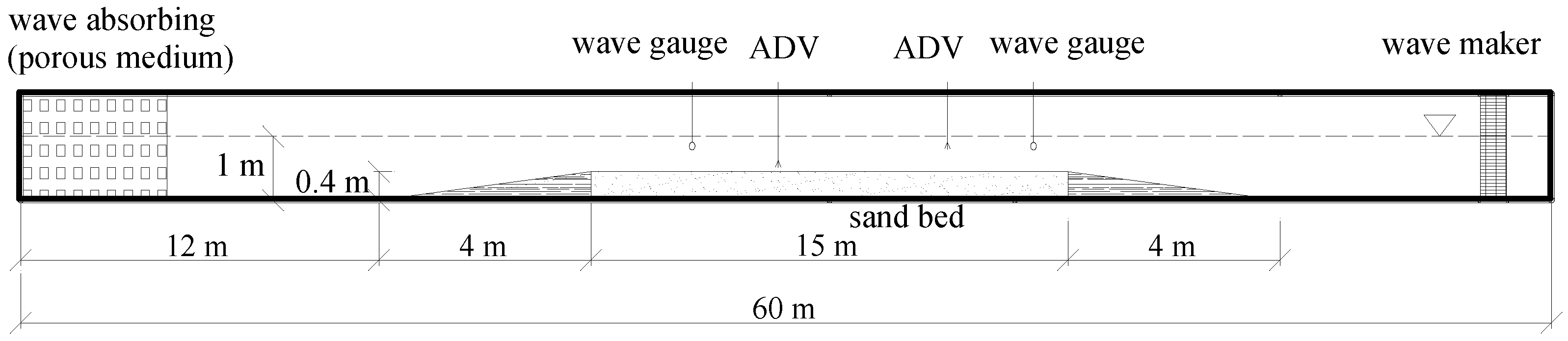
A series of experiments was conducted in the wave-current flume in the Hydraulic Lab at the Ocean University of China. Figure 1 shows the schematic layout of the physical model experiment. The length of the wave flume is 60 m; the height and the width are 1.5 m and 0.8 m, respectively. The waves are generated by a piston type wave maker at one side of the flume. A porous medium is used at the other end to absorb the waves. Uniform currents with positive or negative directions are generated by two circulating pumps. The flume is capable of generating waves of heights between 0.03 m and 0.3 m and wave period between 0.5 s and 3 s. In the middle-rear of the wave flume, the bottom was covered by a sand bed 15 m in length, 0.8 m in width and 0.4 m in thickness with non-cohesive sands. Two 1:10 concrete slopes were set at the both sides of the sand bed to avoid a sudden change of hydrodynamic conditions.
The wave height and wave period are measured with two wave gauges. During the experiments, 50 Hz of sampling rate is used which is sufficient to measure the variation of water surface elevation for all the scenarios in this paper. The depth-averaged velocity is measured by ADV (Acoustic Doppler Velocimetry). The 0.6-depth method (One-point method) is used in the experiments to determine the depth-averaged velocity. A Trasonic Terrain automatic Measurement and analysis System (TTMS) is used to measure evolution of the sand bed. The resolution of the system is ±1 mm in the vertical direction.
The initial bed surface is flat at the beginning of each experiment. Under the waves and currents action, the bed elevation is measured every half an hour in the first hour, and then measured every hour. The experiment is complete when the bed achieves a dynamic equilibrium. In this paper, we assume that the bed has achieved a dynamic equilibrium when the change of bed is less than 5% of the sand wave elevation. Table 1 shows the experimental scenarios. The medium diameter in the first eight tests is 0.17 mm while it is 0.18 mm in the last two tests.
2.2. Water Characteristics Calculation
The Ursell numbers (defined as , here L denotes wave length) computed for all 10 tests in this paper were less than 26. Therefore, small amplitude wave theory can be adopted to obtain the wave configurations. An Ursell number larger than 26 corresponds to shallow water in almost half the cases of Cataño-Lopera et al. [1], so Cnoidal wave theory must be used. Consequently, different wave theories were used according to an Ursell number of 26.
The bed shear stress is an important factor to induce the sediment incipient motion and transport. The dimensionless bed shear stress can be expressed as:
where is mean bed shear stress due to current and waves; is the critical bed shear stress, which is defined as:
where and are the densities of sediment and water, respectively; is gravitational acceleration; is the critical Shields number, which can be calculated according to the classical Shields curve. Here, we adopt a function of the dimensionless particle diameter which is proposed by van Rijn [33]:
where the dimensionless particle diameter is,
where is the viscosity coefficient of water.
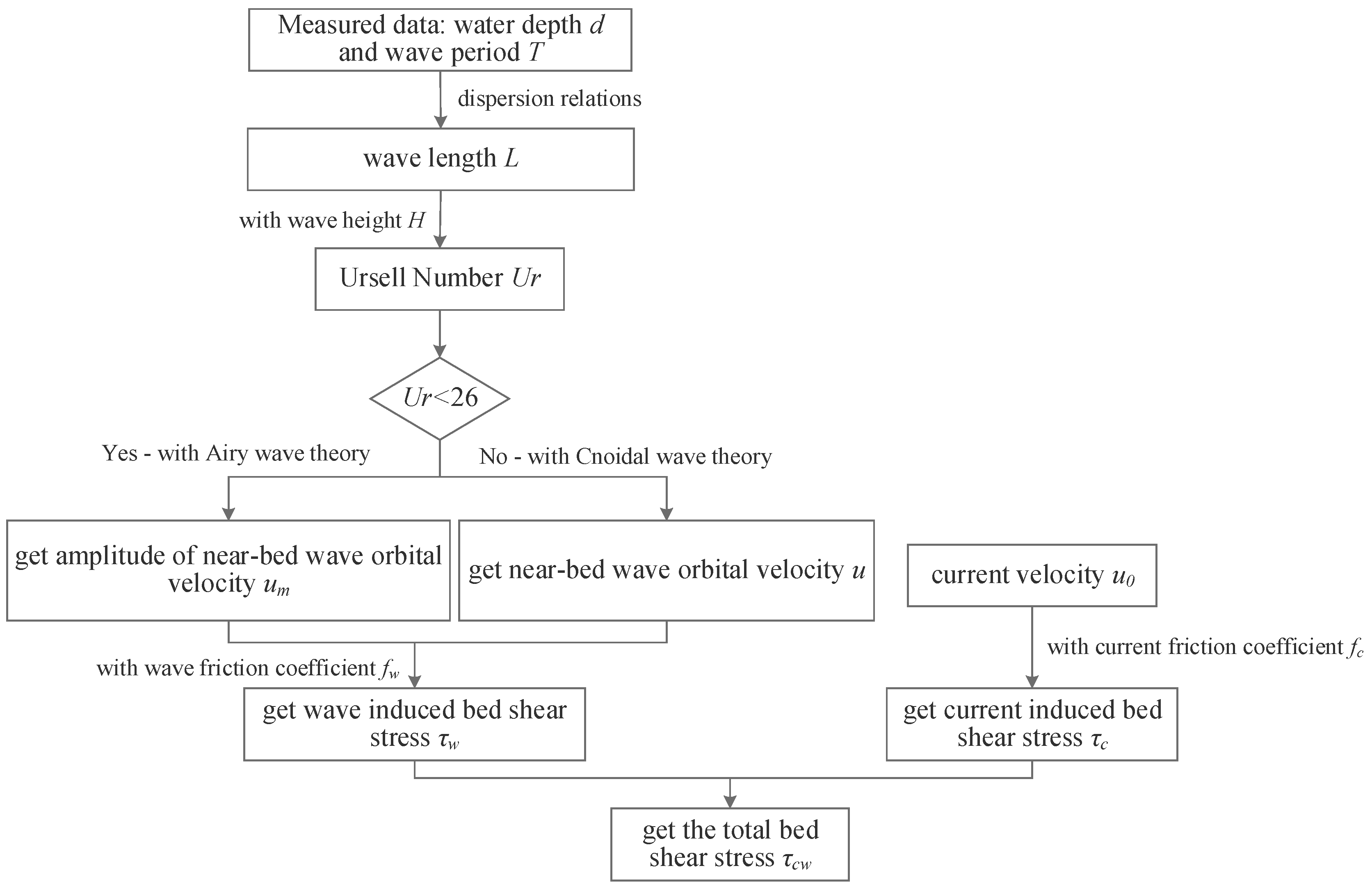
Figure 2 shows the calculation flow chart of total bed shear stress . With the measured wave period and water depth , the wave length is calculated with the dispersion relation,
With the measured wave height , the Ursell number can be obtained. When the Ursell number is less than 26, the amplitude of the near-bottom orbital velocity is calculated according to small amplitude wave theory,
where is the wave number.
The wave-averaged bed shear stress due to waves is calculated as,
where is the wave-related friction factor, which is related to the amplitude of the wave particle and the ripple existing on the bed. We adopt the formulation of Swart [34],
where is the wave related roughness, which is related to the estimated ripple height, , here the ripple height is set as 1.5 cm; is the near-bed peak orbital excursion, which can be solved as,
When the Ursell number is larger than 26, Cnoidal wave theory must be used to evaluate the wave configurations. Based on the Cnoidal wave theory, wave period can be calculated as [35,36]:
where is the modulus of the elliptic integral; and are the first and second types of complete elliptic integrals, respectively. With the measured data of wave period, the parameter of can be solved using the Newton iterative method. Then the wave length with Cnoidal wave theory is:
The time series of the wave particle velocity calculated with Cnoidal wave theory in shallow water is quite different from the small amplitude wave theory. The near-bed instantaneous velocity due to waves can be calculated by:
where , , are Jacobian elliptical sinusoid function and Jacobian elliptical cosine function and Jacobian elliptical delta function, respectively; is the distance from the wave trough to the seabed, the distance from the wave crest to the seabed is defined as .
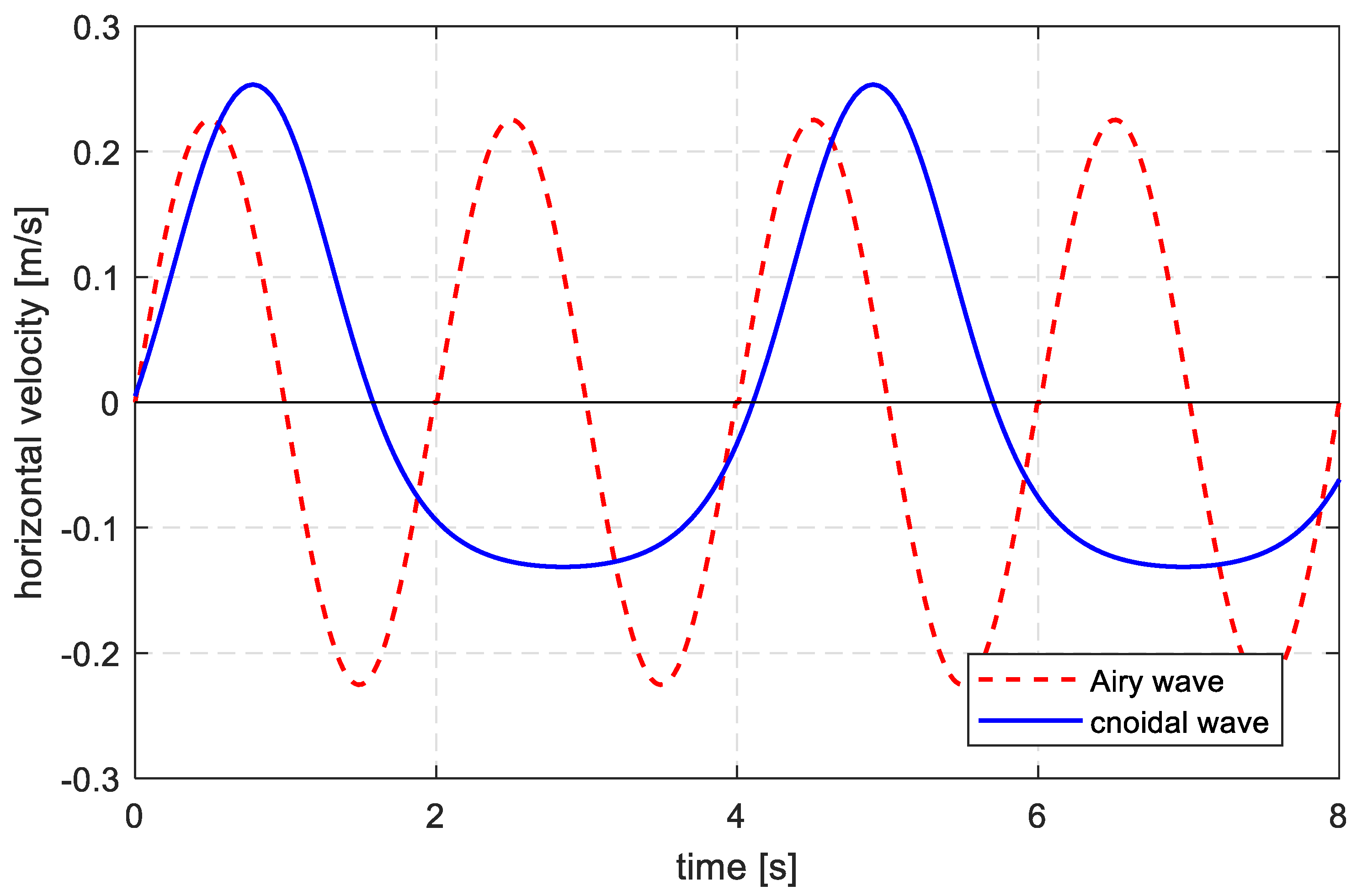
Two scenarios were used to evaluate the difference of velocity between small amplitude wave theory and Cnoidal wave theory. Scenario 3 (with water depth of 0.6 m, wave height of 0.14 m and wave period of 2 s) in Table 1 was used for the first test, while an experimental scenario (with water depth of 0.56 m, wave height of 0.104 m, and wave period of 4.1 s) from Cataño-Lopera et al. [1] was used for the second test. The Ursell numbers for the two tests were 12.33 and 55.5, respectively. Therefore, the small amplitude wave theory was used for the first test and the Cnoidal wave theory was used for the second test. The results can be found in Figure 3.
With Cnoidal wave theory, the wave period-averaged bed shear stress can be expressed as:
It is difficult to get the analytical solution from Equation (18), so a numerical integration method was used. With ,
When the wave is combined with current, the current induced bed shear stress is:
where is the current friction factor. When , can be expressed as [37]:
With all the equations above, the dimensionless bed shear stress can be obtained. Hydrodynamic conditions and characteristics of the measured sand waves are listed in Table 2.
3. Results
3.1. Dynamic Growth of Sand Waves
Take Scenario 4 for example, Figure 4 shows the process of bed evolution during the experiment. First, the bed is flat at the initial time with the help of some calibration lines posted outside the glass of the flume. Second, fill the water into the wave flume until the depth reaches up to 0.6 m upon the sand bed. After the wave action has lasted for several minutes, ripples are formed alternatively on the bed. Third, after about 1-hour’s wave action, the ripples can be found all over the sand bed. Sand waves start to form. Finally, as Figure 4d shows, sand waves are generated. The height of the sand waves is of several centimeters and the length of about several meters. Ripples superimposed upon the sand waves present 2D or 3D patterns depending on their location over the large bedforms. 2D patterns of ripples can often be found at the crest or trough of sand waves, while 3D patterns are often found between the crest and trough. The ripples on the crest are usually larger than those at the trough. It is quite important to investigate the characteristics of ripples at different locations. They can affect the near-bed flow field and bed shear stress dramatically by changing the roughness coefficient.
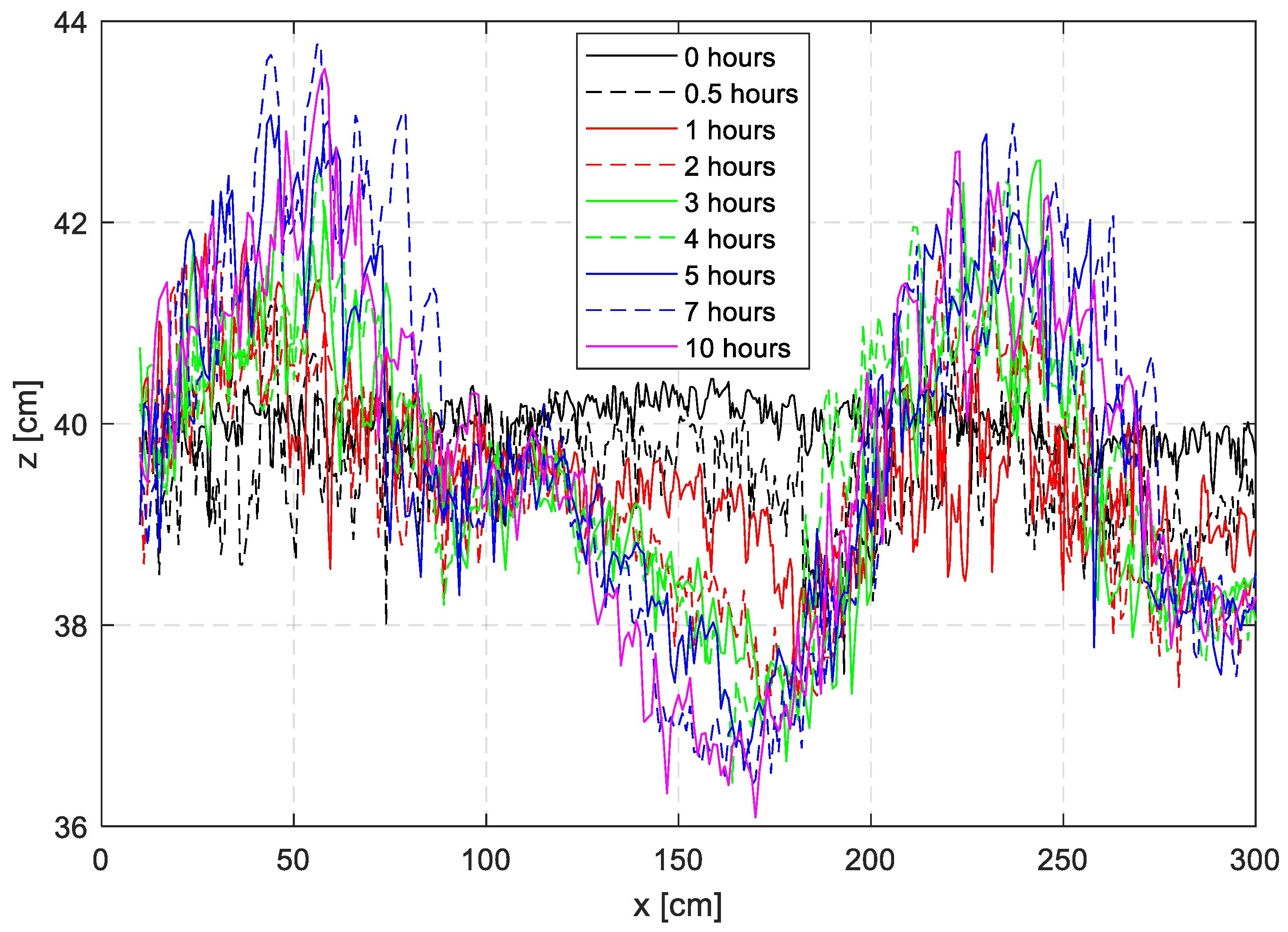
Using the TTMS, the bed level change was measured with an accuracy of 1 cm. Figure 5 shows the bottom evolution over time. With the FFT (Fast Fourier Transformation) method, the wave height can be obtained. In this case, the height of the sand wave is about 3.79 cm, and the length is about 1.78 m after 5 h. Note in Figure 5 the sand wave reaches a quasi-steady condition after 5 h when no obvious bed changes can be observed.
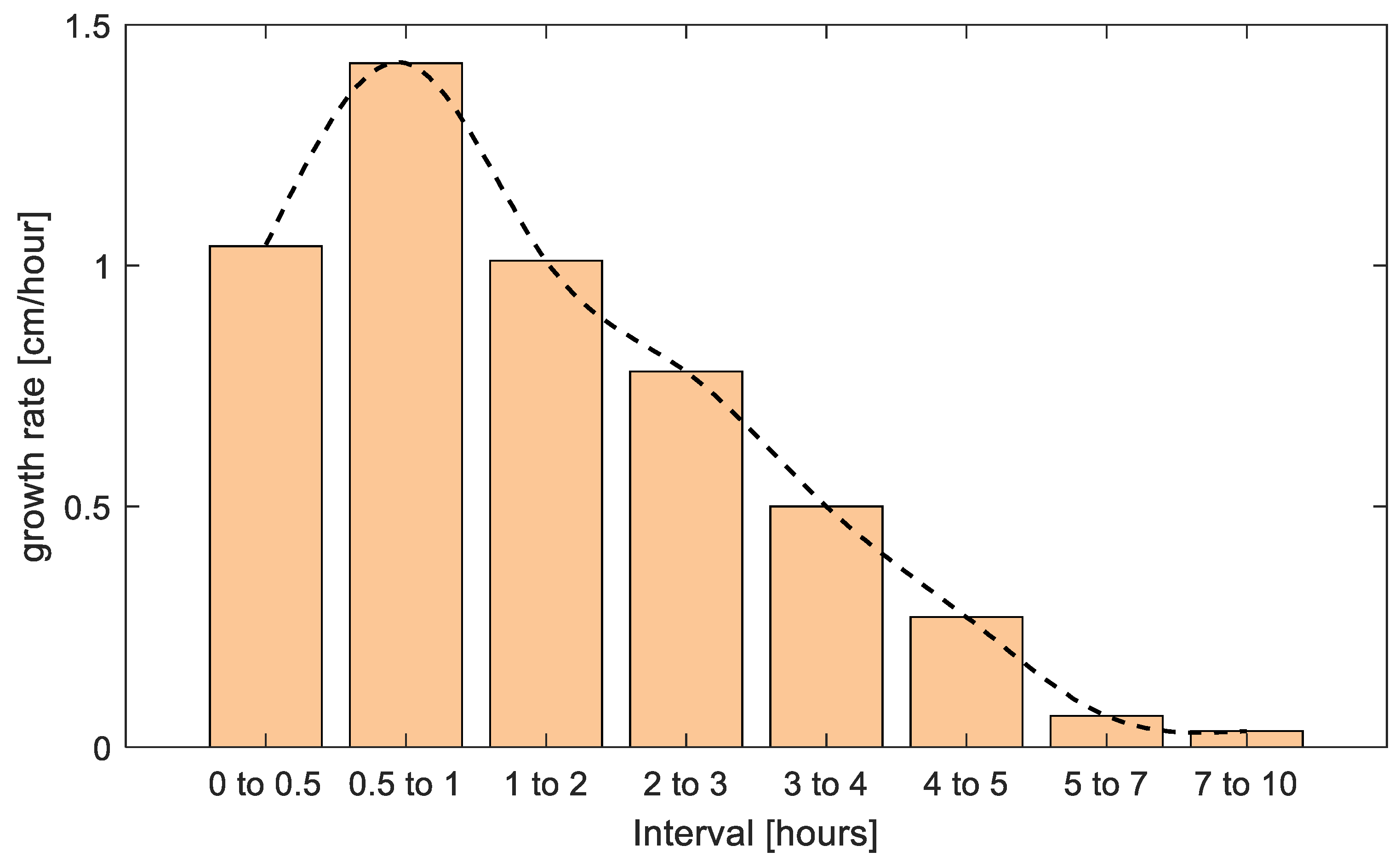
The growth rate of sand waves is calculated with the FFT method of bed level at different times. From Figure 6 the first half hour shows the growth rate is about 1.04 cm/h which is not very large. At this stage ripples start to appear along the bed and large bedforms are formed gradually. The growth rate reaches the largest value which is about 1.42 cm/h in the second half hour and the main geometric characteristics of sand waves begin to be formed. Then from the second to the fifth hour, the growth rate decreases gradually at about 1.01 cm/h, 0.78 cm/h, 0.50 cm/h, and 0.27 cm/h, respectively. The change of bed is less than 5% of the sand wave elevation at the fifth hour, so with the first 5 h wave action the sand waves have reached a balanced state. At an average of 10 h, the growth rate is about 0.4 cm/h.
3.2. Geometry Characteristics of Sand Waves
Dimensionless bed shear stress was used to evaluate the measured sand wave characteristics. The hydrodynamic conditions and measured data of sand waves are listed in Table 2. The measured data of the bed forms denote the long type sand waves, not the ripples superposed on the waves. Notice that Cnoidal wave theory is used when the Ursell number is larger than 26 which make the results more accurate. Figure 7 shows the relationship between dimensionless sand wave height and dimensionless shear stress. The data is rather scattered. A simple linear relationship was used to evaluate change regulation with all the data. The black line is the fitting curve and the formula is as follows.
Dimensionless sand wave height decreases slightly with increase of dimensionless bed shear stress. The correlation coefficient is about 0.02 which shows poor correlation between dimensionless sand wave height and bed shear stress. The data is rather scattered when the dimensionless shear stress is larger than 30, so the hydrodynamic conditions were analyzed. Among these scenarios, the result of Scenario 18 is quite different which is much larger than the others. In addition, the wave steepness of seven scenarios (9, 10, 11, 15, 23, 26, 31) is quite large (larger than 0.04) which is marked by “×” in the figure. Without considering these data, the nonlinear fitting curve is the blue line. The fitting formula can be expressed as,
The correlation coefficient is about 0.49 which was obviously improved. A declining trend can also be found from this formula.
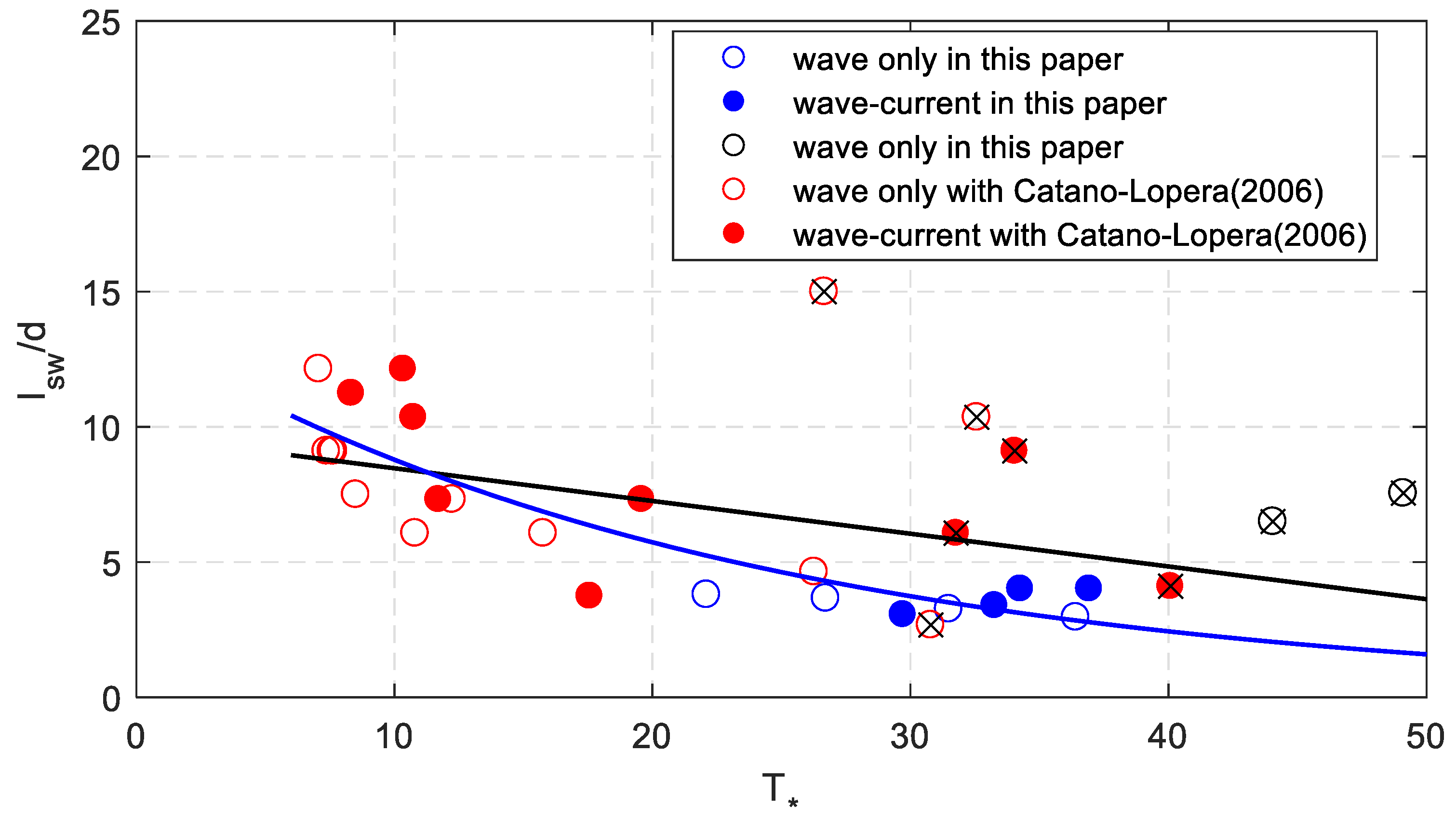
Figure 8 shows the negative relationship between dimensionless sand wave length and dimensionless bed shear stress. The results rather show scatter when all the data are considered. The black line shows the fitting curve with linear relationship and the formula is as follows,
The dimensionless sand wave length decreases with increasing bed shear stress. The correlation coefficient is about 0.47. When the eight tests are not considered, there is a better nonlinear relation (i.e., the blue line in Figure 8). The fitting equation is,
This equation also shows the decline trend of the sand wave length with dimensionless bed shear stress. The correlation coefficient is improved to 0.87. In general, the dimensionless sand wave length decreases with increasing bed shear stress.
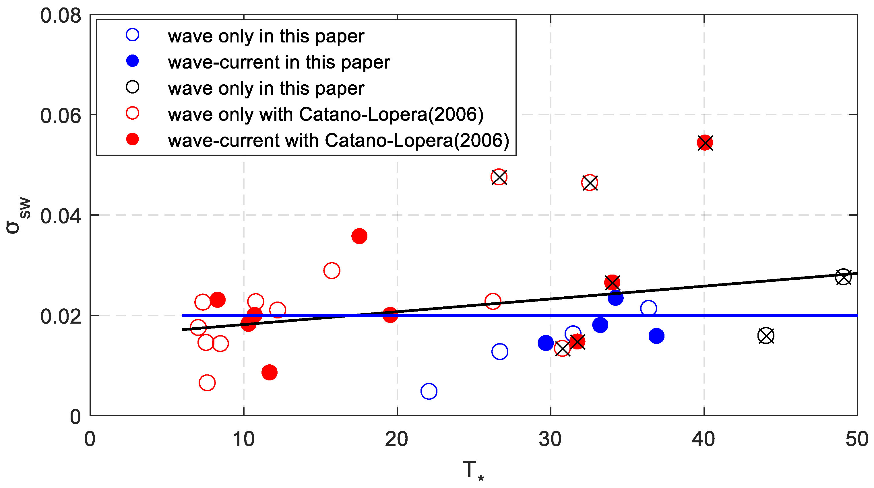
The steepness of sand waves is defined as . As Figure 9 shows, the linear fitting formula can be expressed as follows.
Equation (26) shows that the steepness increases slightly with increase of the dimensionless shear stress. The data seems still rather scattered when the eight larger wave steepnesses of the wave conditions are excluded. However, the sand wave steepness seems to be a constant number which is about 0.02.
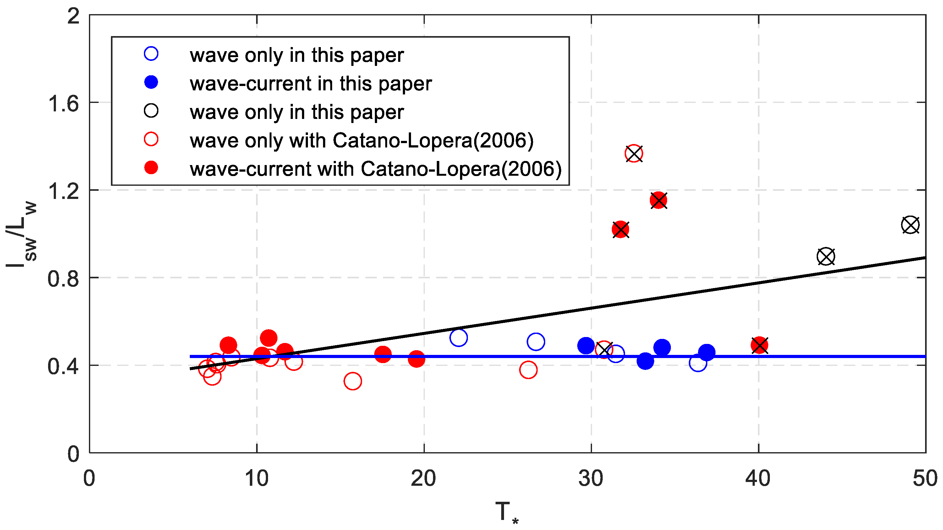
The dimensionless sand wave characteristics above are rather scattered, and here another method was used. The relationship of the dimensionless sand wave length denoted as and the dimensionless shear stress can be found from Figure 10. The black line is the linear fitting line which is,
The correlation coefficient is about 0.44. Excluding the eight tests, a good trend can be found as the blue line. The ratio of sand wave length and wave length is a constant with curve fitting, the value is about 0.44 which corresponds with Cataño-Lopera et al. [1].
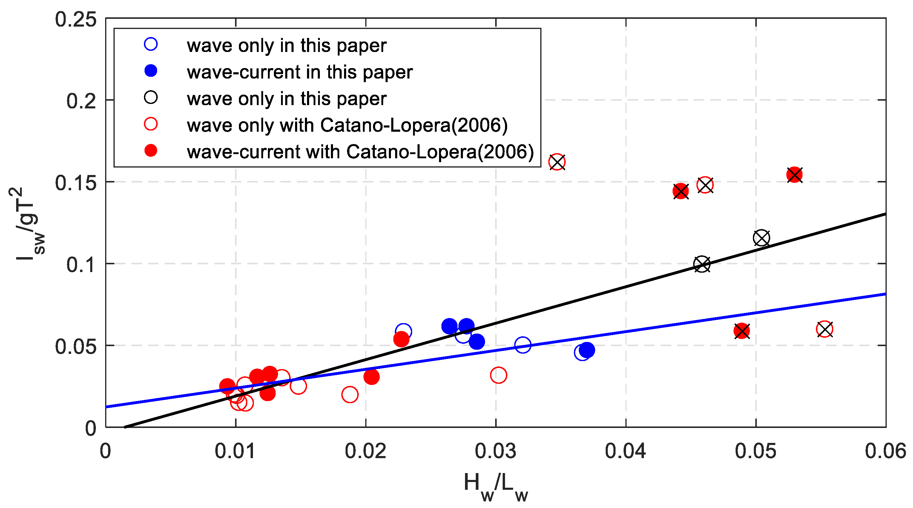
Because of the complication of the calculation of dimensionless shear stress with Cnoidal wave theory in shallow water, the relationship between sand wave length and wave steepness is represented in Figure 11. Considering the large wave steepness, the fitting equation reads,
Without considering the large wave steepness, the fitting equation is (the blue one in Figure 11):
The correlation coefficients are 0.758 and 0.767, respectively. The wave characteristics are easy to obtain, then the sand wave length can be evaluated directly.
4. Discussion
Tidal currents are the most critical environmental factors that control the formation and evolution of sand waves, as confirmed by many field observations and linear stability analyses. In the present study, we argue that waves and currents both have an important effect on sand waves.
4.1. Comparison with the Results of Cataño-Lopera et al. [1]
Cataño-Lopera et al. [1] chose the representative parameter Reynolds wave number (Rew) to express measured values. Twenty one data of tests with waves alone and combined currents were used to analyze the relationship between dimensionless geometric configuration of sand waves and Rew. The wave characteristics were obtained using small amplitude wave theory for all cases though Ursell number was larger than 26 in about half of the experiments. In this paper, Cnoidal wave theory was used to calculate the wave characteristics for the experiments with a large Ursell number. Additionally, two different sediment diameters were used in this paper, and the Reynolds wave number was no longer suitable as the dimensionless parameter because sediment configuration needs to be considered. Therefore, the dimensionless bed shear stress was used as the hydrodynamic parameter in this paper.
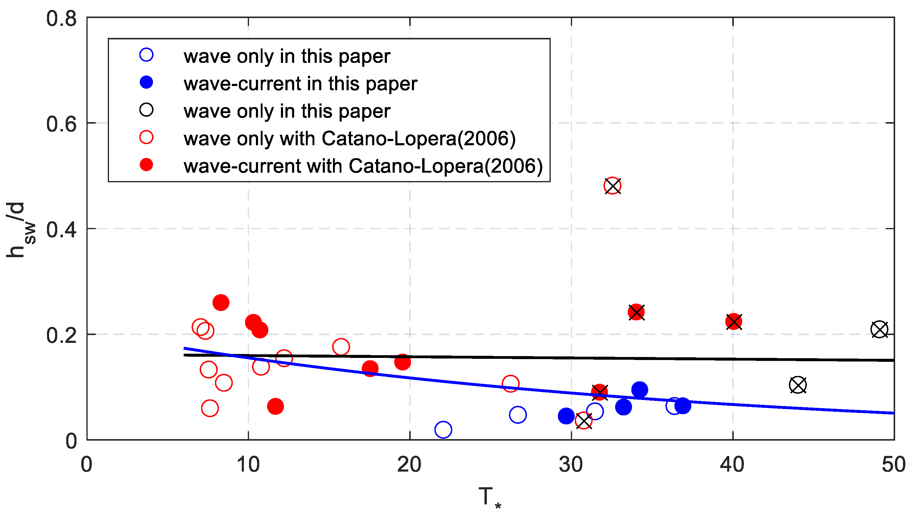
For the cases of Cataño-Lopera, most of the dimensionless shear stress was in the range of 7 to 20, with some data scattered in the range of 30 to 40. The results of our experiments supplement the range of shear stress data in the range from 20 to 30. For dimensionless height and length of sand waves (as Figure 7, Figure 8 and Figure 10 show), they are highly correlated when the dimensionless shear stress is less than 30. The results had poor correlation when the shear stress was larger than 30. According to the wave steepness, the cases larger than 0.04 represent a different trend. Without considering these cases, Equations (23), (25), (29) show good agreement with the measured data.
The measured data is scattered while the wave steepness is large, which may be caused by the wave nonlinearity. When the wave steepness is larger than 0.04, small amplitude wave theory is less accurate in calculating the orbital velocities and bed shear stress. Our equations gave a better relationship for cases when wave steepness was less than 0.04.
4.2. Bedforms with Dimensionless Shear Stress
Sand waves and sand ripples coexist under the waves and currents. Dimensionless shear stress is a key parameter in this paper. According to van Rijn [38], the flow conditions in an alluvial channel are usually classified into: (1) Lower flow regime with plane beds, mini-ripples, mega-ripples, and dunes. (2) Transition flow regime with washed-out dunes and sand waves. (3) Upper flow regime with plane bed or anti-dunes. The upper regime which is defined as occurring for , is characterized by a dominating suspended load transport. It was found from van Rijn [38] that the sand bed would be out of plane and start anti-dunes when the parameter was beyond 25. However, this concept has been challenged by Yalin [39] and Julien [40]. According to their work, lower-regime bedforms can be observed at values of well beyond 25 in very large rivers. Measurements from Table 2 include values of . Sand waves can be found under the upper flow regime of van Rijn. Our experimental results confirmed the findings of Yalin [39] and Julien [40].
Wave energy dissipation and bottom roughness are important parameters in many hydrodynamic and morphodynamic models for coastal oceans, lakes and estuaries [41]. It is important to describe the topography of ripple pattern properly since it determines the net shear stress over the flow field. Xiong et al. [42] calculated the wave height of ripples based on the formulas of Boyd et al. [43] and Allen [44]. The scales are comparable to the results of Zhao et al. [45] at Dongtai. It was found that the ripple-related bottom shear stress is much larger than the skin-friction shear stress. In our experiments, the ripple pattern can be found all over the sand waves. It is reasonable to use Equation (8) to evaluate the roughness.
5. Conclusions
In this paper, a series of experiments was conducted to study sand bed configurations under waves and currents in the wave flume. Both the experimental results of this paper and previous research show that ripples and sand waves coexist together by waves alone and combined currents. Several conclusions can be drawn from the observations and analyses:
(1) Sand ripples can represent 2D patterns or 3D patterns depending on the location of the large-scale sand waves. The 2D ripples existing on the crest are much larger than those on the trough.
(2) Based on the Ursell numbers of different hydrodynamic conditions, the dimensionless bed shear stresses were calculated with different wave theories. Geometry characteristics of sand waves such as height, length, and steepness were very scattered for all cases. Without the cases of large wave steepness, the sand wave height and length both decreased with increase of the dimensionless bed shear stress. The sand wave steepness hardly changed with bed shear stress.
(3) A simple linear relationship can be found between the sand wave length and wave steepness. It is easy to evaluate the sand wave characteristics from the measured wave data.
Author Contributions
Conceptualization, B.L. and Z.W.; methodology, B.L.; formal analysis, Z.W. and B.L.; investigation, Z.W. and G.W.; writing—original draft preparation, Z.W.; writing—review and editing, Z.W. and G.W.; visualization, Z.W.
Funding
This research was funded by National Natural Science Foundation of China, (Grant No. 51679223, 51739010, 51709243).
Acknowledgments
The authors appreciate the comments from the anonymous reviewers.
Conflicts of Interest
The authors declare no conflict of interest.
Notation
The following symbols are used in this paper:
| = wave height |
| = wave period |
| = depth-averaged current velocity |
| = water depth |
| = median diameter of sediment |
| = Ursell number |
| = wave length |
| = dimensionless bed-shear stress |
| = mean bed shear stress due to current and waves |
| = critical bed shear stress |
| = density of sediment |
| = density of water |
| = gravitational acceleration |
| = critical Shields number |
| = dimensionless particle diameter |
| = viscosity coefficient of water |
| = amplitude of the near-bottom wave orbital velocity |
| = wave friction factor |
| = current friction factor |
| = wave-averaged bed shear stress due to waves only |
| = bed shear stress due to current only |
| = wave number |
| = near-bed peak orbital excursion |
| = wave related roughness |
| = ripple height |
| = modulus of elliptic integral |
| = the first kind complete elliptic integral |
| = the second kind complete elliptic integral |
| = near-bed instantaneous velocity due to waves |
| = Jacobian elliptic sinusoid function |
| = Jacobian elliptic cosine function |
| = Jacobian elliptic delta function |
| = distance from the wave trough to the sea bed |
| = distance from the wave crest to the sea bed |
| = sand wave height |
| = sand wave length |
| = sand wave steepness |
References
- Cataño-Lopera, Y.A.; García, M.H. Geometry and migration characteristics of bedforms under waves and currents. Part 1: Sandwave morphodynamics. Coast. Eng. 2006, 53, 767–780. [Google Scholar] [CrossRef]
- Cataño-Lopera, Y.A.; García, M.H. Geometry and migration characteristics of bedforms under waves and currents: Part 2: Ripples superimposed on sandwaves. Coast. Eng. 2006, 53, 781–792. [Google Scholar] [CrossRef]
- Terwindt, J.H.J. Sand waves in the southern bight of the North Sea. Mar. Geol. 1971, 10, 51–67. [Google Scholar] [CrossRef]
- Mccave, I.N. Sand waves in the North Sea off the coast of Holland. Mar. Geol. 1971, 10, 199–225. [Google Scholar] [CrossRef]
- Campmans, G.H.P.; Roos, P.C.; de Vriend, H.J.; Hulshcher, S.J.M.H. Modeling the influence of storms on sand wave formation: A linear stability approach. Cont. Shelf Res. 2017, 137, 103–116. [Google Scholar] [CrossRef]
- Van Dijk, T.A.G.P.; Kleinhans, M.G. Processes controlling the dynamics of compound sand waves in the North Sea, Netherlands. J. Geophys. Res. Earth Surf. 2005, 110, 1–15. [Google Scholar] [CrossRef]
- Besio, G.; Blondeaux, P.; Brocchini, M.; Hulshcer, S.J.M.H.; Idier, D.; Knaapen, M.A.F.; Németh, A.; Roos, P.C.; Vittori, G. The morphodynamics of tidal sand waves: A model overview. Coast. Eng. 2017, 55, 657–670. [Google Scholar] [CrossRef]
- Berg, J.V.D.; Sterlini, F.; Hulscher, S.J.M.H.; Damme, R.V. Non-linear process based modelling of offshore sand waves. Cont. Shelf Res. 2012, 37, 26–35. [Google Scholar] [CrossRef]
- Knaapen, M.A.F.; Hulscher, S.J.M.H.; Tiessen, M.C.H.; Berg, J.V.D.; Parker, G.; García, M.H. Using a sand wave model for optimal monitoring of a navigation depth. In Proceedings of the Forth IAHR Symposium on River, Coastal and Estuarine Morphodynamics, Urbana, IL, USA, 4–7 October 2005; pp. 999–1007. [Google Scholar]
- Németh, A.; Hulscher, S.J.M.H.; de Vriend, H.J. Offshore sand wave dynamics, engineering problems and future solutions. Pipeline Gas J. 2003, 230, 67–69. [Google Scholar]
- Roos, P.C.; Blondeaux, P.; Hulscher, S.J.M.H.; Vittor, G. Linear evolution of sandwave packets. J. Geophys. Res. Earth Surf. 2005, 110, 1–10. [Google Scholar] [CrossRef]
- Ma, X.; Yan, J.; Fan, F. Morphology of submarine barchans and sediment transport in barchans fields off the Dongfang coast in Beibu Gulf. Geomorphology 2014, 213, 213–224. [Google Scholar] [CrossRef]
- Li, Y.; Lin, M.; Jiang, W.; Fan, F. Process control of the sand wave migration in Beibu Gulf of the South China Sea. J. Hydrodyn. 2011, 23, 439–446. [Google Scholar] [CrossRef]
- Dodd, N.; Blondeaux, P.; Calvete, D.; Swart, H.E.D.; Falqués, A.; Hulscher, S.J.M.H.; Różyński, G.; Vittori, G. Understanding coastal morphodynamics using stability methods. J. Coast. Res. 2003, 19, 849–865. [Google Scholar]
- Belderson, R.H. Offshore tidal and non-tidal sand ridges and sheets: Differences in morphology and hydrodynamic setting. In Shelf Sands and Sandstones—Memoir 11; CSPG Special Publications: Calgary, AB, Canada, 1986. [Google Scholar]
- Hulscher, S.J.M.H. Tidal-induced large-scale regular bed form patterns in a three-dimensional shallow water model. J. Geophys. Res. Oceans 1996, 101, 20727–20744. [Google Scholar] [CrossRef]
- Borsje, B.W.; Roos, P.C.; Kranenburg, W.M.; Hulscher, S.J.M.H. Modeling tidal sand wave formation in a numerical shallow water model: The role of turbulence formulation. Cont. Shelf Res. 2013, 60, 17–27. [Google Scholar] [CrossRef]
- Németh, A.A.; Hulscher, S.J.M.H.; de Vriend, H.J. Modelling sand wave migration in shallow shelf seas. Cont. Shelf Res. 2002, 22, 2795–2806. [Google Scholar] [CrossRef]
- Besio, G.; Blondeaux, P.; Brocchini, M.; Vittori, G. On the modeling of sand wave migration. J. Geophys. Res. Oceans 2004, 109, 1–13. [Google Scholar] [CrossRef]
- Campmans, G.H.P.; Roos, P.C.; de Vriend, H.J.; Hulscher, S.J.M.H. The influence of storms on sand wave evolution: A nonlinear idealized modeling approach. J. Geophys. Res. Earth Surf. 2018, 123, 2070–2086. [Google Scholar] [CrossRef]
- Campmans, G.H.P.; Roos, P.C.; Schrijen, E.; Hulscher, S.J.M.H. Modeling wave and wind climate effects on tidal sand wave dynamics: A North Sea case study. Estuar. Coast. Shelf Sci. 2018, 213, 137–147. [Google Scholar] [CrossRef]
- Borsje, B.W.; de Vries, M.B.; Bouma, T.J.; Besio, G.; Hulscher, S.J.M.H.; Herman, P.M.J. Modelling biogeomorphological influences for offshore sandwaves. Cont. Shelf Res. 2009, 29, 1289–1301. [Google Scholar] [CrossRef]
- Borsje, B.W.; Hulscher, S.J.M.H.; Herman, P.M.J.; de Vries, M.B. On the parameterization of biological influences on offshore sandwave dynamics. Ocean Dyn. 2009, 59, 659–670. [Google Scholar] [CrossRef]
- Roos, P.C.; Wemmenhove, R.; Hulscher, S.J.M.H.; Hoeijmakers, H.W.M.; Kruyt, N.P. Modeling the effect of nonuniform sediment on the dynamics of offshore tidal sandbanks. J. Geophys. Res. Earth Surf. 2007, 112, 1–11. [Google Scholar] [CrossRef]
- Van Oyen, T.; Blondeaux, P. Grain sorting effects on the formation of tidal sand waves. J. Fluid Mech. 2009, 629, 311–342. [Google Scholar] [CrossRef]
- Van Oyen, T.; Blondeaux, P. Tidal sand wave formation: Influence of graded suspended sediment transport. J. Geophys. Res. Oceans 2009, 114, 1–18. [Google Scholar] [CrossRef]
- Blondeaux, P. Sediment mixtures, coastal bedforms and grain sorting phenomena: An overview of the theoretical analyses. Adv. Water Resour. 2012, 48, 113–124. [Google Scholar] [CrossRef]
- Borsje, B.W.; Kranenburg, W.M.; Roos, P.C.; Matthieu, J.; Hulscher, S.J.M.H. The role of suspended load transport in the occurrence of tidal sand waves. J. Geophys. Res. Earth Surf. 2014, 119, 701–716. [Google Scholar] [CrossRef]
- Van Gerwen, W.; Borsje, B.W.; Damveld, J.H.; Hulscher, S.J.M.H. Modelling the effect of suspended load transport and tidal asymmetry on the equilibrium tidal sand wave height. Coast. Eng. 2018, 136, 56–64. [Google Scholar] [CrossRef]
- Chou, Y.J.; Shao, Y.C.; Sheng, Y.H.; Cheng, C.J. Stabilized formulation for modeling the erosion/deposition flux of sediment in circulation/CFD models. Water 2019, 11, 197. [Google Scholar] [CrossRef]
- Williams, J.J.; Bell, P.S.; Thorne, P.D. Unifying large and small wave-generated ripples. J. Geophys. Res. Oceans 2005, 110, 1–18. [Google Scholar] [CrossRef]
- Zhu, X.; Wang, Z.; Wu, Z.; Liu, F.; Liang, B.; He, Y.; Huang, F. Experiment research on geometry and evolution characteristics of sand wave bedforms generated by waves and currents. In 5th International Conference on Coastal and Ocean Engineering, Shanghai, China, 2018; IOP Conference Series: Earth and Environmental Science; IOP Publishing: Bristol, UK, 2018; pp. 9–15. [Google Scholar]
- Van Rijn, L.C. Principles of Sediment Transport in Rivers, Estuaries and Coastal Seas; Aqua Publications: Blokzijl, The Netherlands, 1993. [Google Scholar]
- Swart, D.H. Offshore Sediment Transport and Equilibrium Beach Profiles. Ph.D. Thesis, Civil Engineering and Geosciences, Delft, The Netherlands, December 1974. [Google Scholar]
- Korteweg, D.J.; de Vries, G. On the change of form of long waves advancing in a rectangular canal, and on a new type of stationary waves. Lond. Edinb. Dublin Philos. Magazine J. Sci. 1895, 39, 422–443. [Google Scholar] [CrossRef]
- Keller, J.B. The solitary wave and periodic waves in shallow water. Commun. Appl. Math. 1984, 1, 323–339. [Google Scholar] [CrossRef]
- Zou, Z.L. Coastal Dynamics; China Communications Press: Beijing, China, 2009. (In Chinese) [Google Scholar]
- Van Rijn, L.C. Sediment transport, part III: Bed forms and alluvial roughness. J. Hydraul. Eng. ASCE 1984, 110, 1733–1754. [Google Scholar] [CrossRef]
- Yalin, M.S. River Mechanics; Pergamon Press: Oxford, UK, 1992. [Google Scholar]
- Julien, P.Y. Erosion and Sedimentation; Cambridge University Press: Cambridge, UK, 2010. [Google Scholar]
- Wiberg, P.L.; Sherwood, C.R. Calculating wave-generated bottom orbital velocities from surface-wave parameters. Comput. Geosci. 2008, 34, 1243–1262. [Google Scholar] [CrossRef]
- Xiong, J.; Wang, Y.P.; Gao, S.; Du, J.; Yang, Y.; Tang, J.; Gao, J. On estimation of coastal wave parameters and wave-induced shear stresses. Limnol. Oceanogr. Meth. 2018, 16, 594–606. [Google Scholar] [CrossRef]
- Boyd, R.; Forbes, D.L.; Heffler, D.E. Time-sequence observations of wave-formed sand ripples on an ocean shoreface. Sedimentology 1988, 35, 449–464. [Google Scholar] [CrossRef]
- Allen, J.R.L. Physical Processes of Sedimentation; American Elsevier Pub. Co.: New York, NY, USA, 1970. [Google Scholar]
- Zhao, N.; Liu, X.J.; Lu, G. Characteristics and evolution process and their modeling of sand ripples on Dongtai tidal flats, Jiangsu province China. J. Sediment. Res. 2012, 3, 4, (In Chinese with English abstract). [Google Scholar]
Figure 1.
Schematic diagram of model experimental layout.

Figure 2.
Flow chart to calculate the total bed shear stress.

Figure 3.
Time series of the wave particle horizontal velocity with different wave theories. The red dash line represents the first test and the wave velocity is symmetrical in a wave period. The blue solid line represents the second test and the wave velocity is larger following the wave direction but the duration is shorter.

Figure 4.
Bed evolution over time during the experiment. (a) initial time; (b) several minutes later; (c) 1 h later; (d) 10 h later.
Figure 4.
Bed evolution over time during the experiment. (a) initial time; (b) several minutes later; (c) 1 h later; (d) 10 h later.

Figure 5.
Bottom evolution over time: the generation of a sand wave.

Figure 6.
The growth rate of a sand wave as a function of time.

Figure 7.
The relationship between the measured dimensionless sand wave height and dimensionless shear stress. The blue circles represent the results of experiments of this paper with a medium diameter of 0.17 mm and the dark ones of 0.18 mm. The red circles represent the results of experiments conducted by Cataño-Lopera et al. [1]. The range of the dimensionless shear stress is about 7–49.

Figure 8.
The relationship between the measured dimensionless sand wave length and dimensionless shear stress.
Figure 8.
The relationship between the measured dimensionless sand wave length and dimensionless shear stress.

Figure 9.
The relationship between the measured sand wave steepness and dimensionless shear stress. The black line is the fitting curve for all the data.
Figure 9.
The relationship between the measured sand wave steepness and dimensionless shear stress. The black line is the fitting curve for all the data.

Figure 10.
The relationship between the measured dimensionless sand wave length and dimensionless shear stress.
Figure 10.
The relationship between the measured dimensionless sand wave length and dimensionless shear stress.

Figure 11.
The relationship between the measured dimensionless sand wave height and dimensionless wave length.
Figure 11.
The relationship between the measured dimensionless sand wave height and dimensionless wave length.


Table 1.
Experimental scenarios.
| Scenarios | H (m) | T (s) | u0 (m/s) | d (m) | D50 (mm) |
|---|---|---|---|---|---|
| 1 | 0.10 | 2 | 0 | 0.6 | 0.17 |
| 2 | 0.12 | 2 | 0 | 0.6 | 0.17 |
| 3 | 0.14 | 2 | 0 | 0.6 | 0.17 |
| 4 | 0.16 | 2 | 0 | 0.6 | 0.17 |
| 5 | 0.14 | 2 | −0.2 | 0.6 | 0.17 |
| 6 | 0.14 | 2 | 0.2 | 0.6 | 0.17 |
| 7 | 0.14 | 2 | 0.25 | 0.6 | 0.17 |
| 8 | 0.14 | 2 | 0.35 | 0.6 | 0.17 |
| 9 | 0.20 | 2 | 0 | 0.6 | 0.18 |
| 10 | 0.22 | 2 | 0 | 0.6 | 0.18 |
Where H is wave height; T is wave period; u0 is depth-averaged current velocity; d is the water depth, and D50 is the median diameter of sediment.
Table 2.
Hydrodynamic conditions and characteristics of measured sand waves.
| Scenarios a | H (cm) | T (s) | u0 (m/s) | d (m) | D50 (mm) | hsw (cm) | lsw (m) | Ur | ||||
|---|---|---|---|---|---|---|---|---|---|---|---|---|
| 1 | 10.0 | 2 | 0 | 0.6 | 0.17 | 1.09 | 2.28 | 8.81 | 3.49 | 0.00 | 0.15 | 22.10 |
| 2 | 12.0 | 2 | 0 | 0.6 | 0.17 | 2.79 | 2.2 | 10.57 | 4.19 | 0.00 | 0.15 | 26.72 |
| 3 | 14.0 | 2 | 0 | 0.6 | 0.17 | 3.18 | 1.96 | 12.33 | 4.92 | 0.00 | 0.15 | 31.49 |
| 4 | 16.0 | 2 | 0 | 0.6 | 0.17 | 3.79 | 1.78 | 14.09 | 5.66 | 0.00 | 0.15 | 36.41 |
| 5 | 14.0 | 2 | −0.2 | 0.6 | 0.17 | 2.65 | 1.84 | 12.33 | 4.92 | −0.27 | 0.15 | 29.71 |
| 6 | 14.0 | 2 | 0.2 | 0.6 | 0.17 | 3.67 | 2.04 | 12.33 | 4.92 | 0.27 | 0.15 | 33.26 |
| 7 | 14.0 | 2 | 0.25 | 0.6 | 0.17 | 5.64 | 2.41 | 12.33 | 4.92 | 0.42 | 0.15 | 34.26 |
| 8 | 14.0 | 2 | 0.35 | 0.6 | 0.17 | 3.81 | 2.41 | 12.33 | 4.92 | 0.82 | 0.15 | 36.93 |
| 9 | 20.0 | 2 | 0 | 0.6 | 0.18 | 6.2 | 3.9 | 17.62 | 7.22 | 0.00 | 0.16 | 44.05 |
| 10 | 22.0 | 2 | 0 | 0.6 | 0.18 | 12.5 | 4.53 | 19.38 | 8.03 | 0.00 | 0.16 | 49.10 |
| 11 | 19.6 | 2 | 0 | 0.56 | 0.25 | 26.9 | 5.8 | 20.12 | 7.47 | 0.00 | 0.22 | 32.57 |
| 12 b | 12.8 | 5.2 | 0 | 0.56 | 0.25 | 3.3 | 5.1 | 117.19 | 1.93 | 0.00 | 0.22 | 7.65 |
| 13 | 19.2 | 6.9 | 0 | 0.56 | 0.25 | 11.9 | 6.8 | 347.56 | 1.80 | 0.00 | 0.22 | 7.07 |
| 14 | 19.7 | 4.2 | 0 | 0.56 | 0.25 | 9.8 | 3.4 | 123.08 | 3.73 | 0.00 | 0.22 | 15.77 |
| 15 | 17.7 | 1.6 | 0 | 0.56 | 0.25 | 2 | 1.5 | 10.32 | 7.08 | 0.00 | 0.22 | 30.79 |
| 16 | 20.9 | 2.9 | 0 | 0.56 | 0.25 | 5.9 | 2.6 | 56.76 | 6.07 | 0.00 | 0.22 | 26.27 |
| 17 | 10.7 | 3.4 | 0 | 0.56 | 0.25 | 7.7 | 3.4 | 37.88 | 2.63 | 0.00 | 0.22 | 10.81 |
| 18 | 17.4 | 2.3 | 0 | 0.56 | 0.25 | 39.9 | 8.4 | 24.83 | 6.16 | 0.00 | 0.22 | 26.66 |
| 19 | 15.1 | 5.9 | 0 | 0.56 | 0.25 | 11.5 | 5.1 | 186.26 | 1.86 | 0.00 | 0.22 | 7.37 |
| 20 | 10.4 | 4.1 | 0 | 0.56 | 0.25 | 6 | 4.2 | 55.46 | 2.12 | 0.00 | 0.22 | 8.51 |
| 21 | 14.7 | 4.1 | 0 | 0.56 | 0.25 | 8.6 | 4.1 | 82.12 | 2.95 | 0.00 | 0.22 | 12.24 |
| 22 | 12.3 | 5.1 | 0 | 0.56 | 0.25 | 7.4 | 5.1 | 107.38 | 1.91 | 0.00 | 0.22 | 7.57 |
| 23 | 19.6 | 1.9 | 0.17 | 0.56 | 0.25 | 13.5 | 5.1 | 17.75 | 7.60 | 0.20 | 0.22 | 34.04 |
| 24 | 19.2 | 5.8 | 0.17 | 0.56 | 0.25 | 12.4 | 6.8 | 240.36 | 2.32 | 0.20 | 0.22 | 10.34 |
| 25 | 19.7 | 3.7 | 0.17 | 0.56 | 0.25 | 8.2 | 4.1 | 92.73 | 4.38 | 0.20 | 0.22 | 19.58 |
| 26 | 17.7 | 1.5 | 0.17 | 0.56 | 0.25 | 5 | 3.4 | 8.65 | 7.10 | 0.20 | 0.22 | 31.77 |
| 27 | 11.3 | 3.6 | 0.17 | 0.56 | 0.25 | 3.5 | 4.1 | 45.68 | 2.63 | 0.20 | 0.22 | 11.71 |
| 28 | 10.7 | 2 | 0.17 | 0.56 | 0.25 | 7.5 | 2.1 | 10.98 | 3.93 | 0.20 | 0.22 | 17.57 |
| 29 | 12.1 | 5.1 | 0.17 | 0.56 | 0.25 | 14.5 | 6.3 | 105.38 | 1.88 | 0.20 | 0.22 | 8.33 |
| 30 | 13 | 4.4 | 0.17 | 0.56 | 0.25 | 11.6 | 5.8 | 83.15 | 2.41 | 0.20 | 0.22 | 10.74 |
| 31 | 23 | 2 | 0.17 | 0.56 | 0.25 | 12.5 | 2.3 | 23.61 | 8.95 | 0.20 | 0.22 | 40.08 |
a The first 10 scenarios were conducted in this paper, the last 21 scenarios were conducted by Cataño-Lopera et al. [1]. b The rows with brown color denote the shallow water, with Cnoidal wave theory.
© 2019 by the authors. Licensee MDPI, Basel, Switzerland. This article is an open access article distributed under the terms and conditions of the Creative Commons Attribution (CC BY) license (http://creativecommons.org/licenses/by/4.0/).
Share and Cite
MDPI and ACS Style
Wang, Z.; Liang, B.; Wu, G. Experimental Investigation on Characteristics of Sand Waves with Fine Sand under Waves and Currents. Water 2019, 11, 612. https://doi.org/10.3390/w11030612
AMA Style
Wang Z, Liang B, Wu G. Experimental Investigation on Characteristics of Sand Waves with Fine Sand under Waves and Currents. Water. 2019; 11(3):612. https://doi.org/10.3390/w11030612
Chicago/Turabian StyleWang, Zhenlu, Bingchen Liang, and Guoxiang Wu. 2019. "Experimental Investigation on Characteristics of Sand Waves with Fine Sand under Waves and Currents" Water 11, no. 3: 612. https://doi.org/10.3390/w11030612
Note that from the first issue of 2016, this journal uses article numbers instead of page numbers. See further details here.