Centrifugal Modeling and Validation of Solute Transport within Unsaturated Zone

Abstract

Numerical modeling has been adopted to assess the feasibility of centrifugal simulation of solute transport within the unsaturated zone. A numerical model was developed to study the centrifugal simulation of nonreactive, adsorption, radionuclide, and reactive solutes. The results showed that it is feasible to conduct centrifugal experiments for nonreactive solute transport. For the solute transport containing physical processes or chemical reactions, if the reaction is very rapid or slow, it is feasible to conduct centrifugal experiments. For the solute transport with a product B generated, if the reaction is relatively slow, the centrifugal prediction of solute is suitable. The centrifugal prediction of solute A matches the prototype quite well, but the prediction of B is in poor quality. If B is the focus, it is not feasible to conduct centrifugal experiments; but if B is not important, the centrifugal modeling is suitable. This has significant implications for the centrifugal modeling application to solute transport simulation within the unsaturated zone.

1. Introduction

Generally speaking, water within the unsaturated zone is under less than atmospheric pressure, and some of the voids may contain air or other gases at atmospheric pressure. This zone is the region where the meteoric and surface water link and exchange moisture with the groundwater. Therefore, the unsaturated zone is the channel that the surface contaminant transports downward to pollute the soil and groundwater. As it is a complex system where three phases of soil, water, and air coexist, both flow and contaminant transport in the unsaturated zone are characterized by complexities that do not exist in the saturated zone [1]. The effective groundwater pollution prevention and control strategies can be made based on the understanding and systematic study of the unsaturated solute transport.

It is widely accepted that the combination of physical modeling and numerical simulation is an effective way to study solute transport within the unsaturated zone [2]. Since the 1980s, this study has begun based on the study of flow in the unsaturated zone. Three methods, including indoor soil column experiment, field experiment, and numerical analysis, have been adopted to study unsaturated solute transport. There are many indoor column and field experiment studies of unsaturated solute transport, mainly including: (1) study solute transport laws through both the concentration curves and the numerical model [3,4]; (2) determinate the transport parameters (dispersion coefficient, diffusion coefficient, and adsorption parameter) and their influence on solute transport [5,6]; (3) develop numerical models to simulate unsaturated solute transport, such as Hydrus, VS2D (a graphical software package for simulating fluid flow and solute or energy transport in variably saturated and unsaturated porous media), and so on. Numerical models have been improved much from simple analytical models to complex numerical solutions, from traditional convection-diffusion model to reaction-transport model, and coupled unsaturated zone-saturated zone models. The initial and boundary conditions have also been improved to be more close to the actual situation of unsaturated solute transport.

In order to further understand the complex unsaturated processes, centrifugal modeling has been used since the 1980s [7,8]. It has many advantages compared to traditional physical models [9]: (1) the experimental data can be collected rapidly; (2) the consistent stress level with the prototype can be accessed; (3) it can predict the full-scale prototype behavior from the centrifugal model; (4) 2- and 3-dimensional models with appropriate boundary conditions are allowed. In recent years, this technology has successfully been applied to study the flow processes [10,11] and solute transport of various materials [12,13,14] in the unsaturated zone.

Since the small size of the centrifugal model can represent the large size of the prototype, in order to make the experiment closer to the actual situation and make the data of both the prototype and the centrifugal model to have good comparability, the height of the prototype planned to be constructed is 5 m. The column of the prototype is made of polymethyl methacrylate, with an effective height of 4.5 m and an inner diameter of 0.9 m. There are 10 sampling and monitoring holes on the column body, and the arrangement of the holes is dense at both ends (used to monitor the transport characteristics at the early stage of solute migration) and sparse in the middle (used to monitor the transport characteristics of solute in the potential capillary zone at the bottom). Two large soil columns were filled to verify the repeatability of the experiment. At the bottom of each soil column, a 30 cm thick gravel layer was first filled to ensure the free infiltration of water. A space of 20 cm was reserved at the top of the soil column for the arrangement of water supply devices. The soil column was filled in layers evenly, and the layers were roughened to ensure homogeneity.

The centrifuge used in the centrifugal modeling has two types: geotechnical centrifuge (large-medium type) and miniature centrifuge. The former has been applied more widely than the latter due to its bigger operating space, more control variables, and dynamic data acquisition through certain technological means. The geotechnical centrifuge is often used for model simulations with multiple simulation objects, from inert metal ions [15] to heavy metal ions [16], and non-aqueous phase liquids (NAPLs) [17,18]. Recently, the geotechnical centrifuge is used to study the heterogeneity’s influence on unsaturated solute transport [19], solute transport in the clay aquitard [20], and the pollutant removal [20]. The miniature centrifuge has been used for the centrifugal tests of soil characteristic parameters, such as the saturated permeability coefficient, soil water characteristic curve, and so on. Lately, the miniature centrifuge has been applied in the micro-scale unsaturated solute transport [21], but these centrifugal experiments are limited to the small size and homogeneous samples.

The chief objective of this study was to offer a new approach to verify whether it’s feasible to apply the centrifugal modeling to the unsaturated solute transport. A one-dimensional solute transport numerical model in the unsaturated zone was established using centrifugal modeling. Then, the behavior characteristics of nonreactive, adsorption, and radioactive nuclide solutes, as well as the applicable conditions of the centrifugal modeling, were comprehensively analyzed.

2. Centrifugal Experiment Modeling

2.1. Centrifugal Similarity Theory

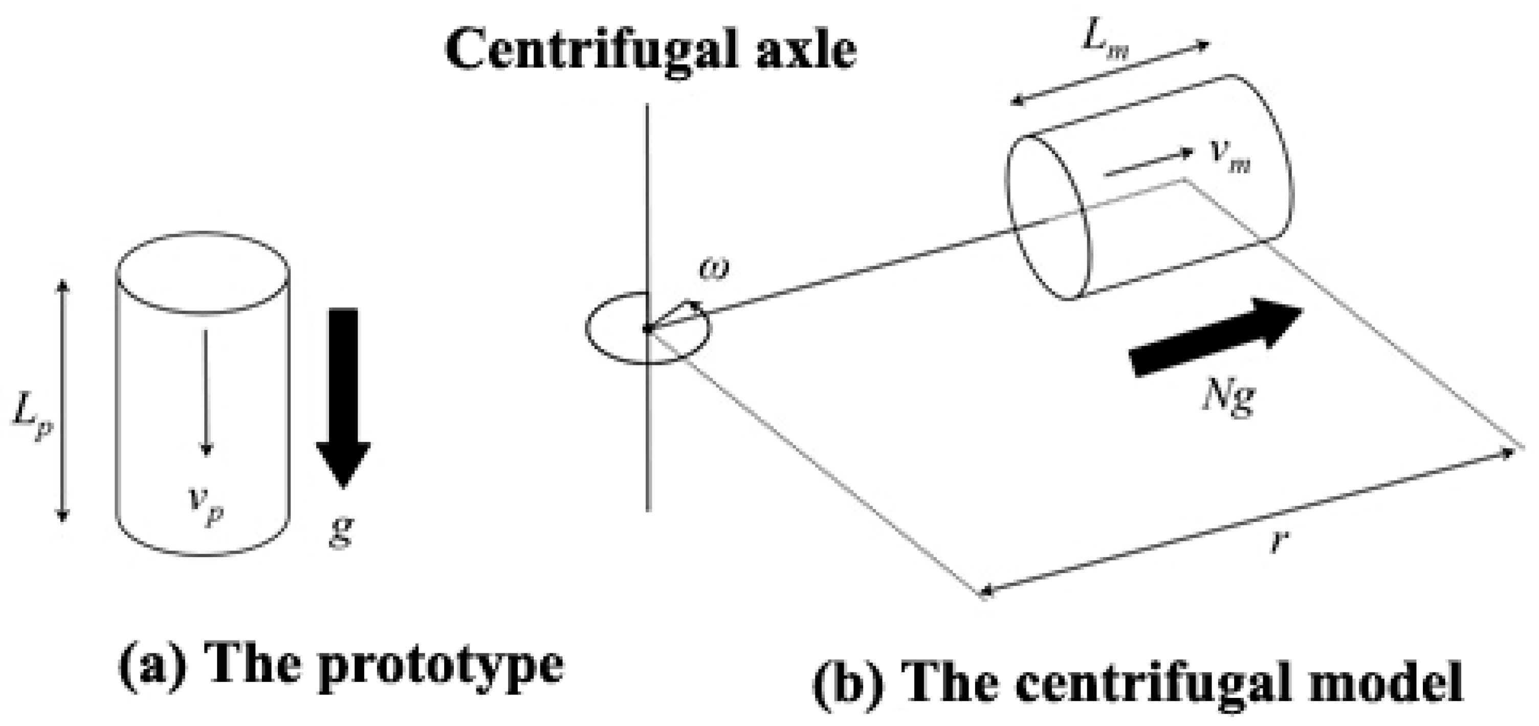
The centrifugal experiment modeling conceptualized in Figure 1 refers to the modeling technology that recovers the stress level of the scaled-down prototype (being called centrifugal model hereafter) installed in the centrifuge by the centrifugal acceleration [22]. An appropriate similarity ratio, which has three types, including geometric, motion, and dynamic similarity ratios, converts the small scale model into the prototype to characterize the prototype [7,22].

The geometric similarity ratio, which ensures the centrifugal model and the prototype have the same stress levels at the corresponding points, is the basic one of the centrifugal modeling. If the soil and osmotic solution in the prototype and the centrifugal model are the same, the stresses at the l_p depth of the prototype soil and at the l_m depth of the corresponding centrifugal model are:

$${\delta }_p={\rho }_{p}g{l}_p$$

(1)

$${\delta }_m={\rho }_m(Ng)l_m$$

(2)

where ρ_p and ρ_m are the soil density of the prototype and the centrifugal model, respectively, g is the gravitational acceleration, and Ng represents that the centrifugal experiment is carried out under the acceleration of Ng. N is also called the gravity level (g-level).

As the prototype and the centrifugal model have the same soil and osmotic solution, that is, ρ_p = ρ_m, there is a relationship between the geometric sizes of them:

$$\frac{l_m}{l_p}=\frac{1}{N}$$

(3)

The motion similarity is based on the geometric similarity with the similar seepage velocity and acceleration [7,22]:

$$\frac{v_m}{v_p}=N$$

(4)

$$\frac{a_m}{a_p}=N$$

(5)

where v_m and v_p, and a_m and a_p are the seepage velocities and accelerations of the centrifugal model and the prototype, respectively; a_p = g.

The dynamic similarity ensures a fixed ratio in the forces and rate constants of the physical and chemical process in the centrifugal model and the prototype:

$$\frac{{\left(F_i\right)}_m}{{\left(F_i\right)}_p}=\alpha$$

(6)

where F represents a variety of force forms (weight, viscosity, pressure, etc.) or the rate constant created by the physical and chemical processes; α is a constant; the subscript m and p represent the centrifugal model and the prototype, respectively.

A series of similarity ratios of physical and chemical parameters can be derived in the process of simulating the same prototype using centrifugal modeling technology (

Table 1. The similarity ratios of the centrifugal experiment modeling (the same soil and osmotic solution are used in the prototype and the centrifugal model).

Symbol	Physical Meaning	Dimension	Similarity Ratio (the Same Prototype)	Similarity Ratio (the Same Centrifugal Model)
a	Centrifugal acceleration	LT−2	N	N
σ	Stress	ML−1T−2	1	N
C	Pollutant concentration	ML−3	1	1
v	Fluid velocity	LT−1	N	N
k	Permeability	L2	1	1
K	Hydraulic conductivity	LT−1	N	N
μ	Fluid viscosity	ML−1T−1	1	1
T	Surface tension	MT−2	1	1
D	Hydrodynamic dispersion coefficient	L2T−1	If Pe < 1, 1; If Pe > 1, N	If Pe < 1, 1; If Pe > 1, N
DD	Molecular diffusivity coefficient	L2T−1	1	1
L	Macro-size	L	1/N	1
d	Micro-size	L	1	1
ρ	Liquid density	ML−3	1	1
Kd	Adsorption coefficient	ML−3	1	1
kr	Chemical reaction rate	T−1	1	1
t	Time	T	1/N2	1/N

). The time needed by the centrifugal modeling is 1/N² of the prototype needs, namely, it only needs less than 4 days to simulate 100 years’ transport of the prototype under the acceleration of 100 g. This characteristic is the main reason for this technology to be widely used. The acceleration of the centrifugal model is a distribution one rather than a fixed value in the radial direction as it is related to the radius and angular velocity. Therefore, the distributed acceleration will result in a little different stress compared with the prototype, which will cause an error between the centrifugal model and the prototype. Taylor [23] pointed out that the minimum error would be obtained if the stress values at 2/3 height of the centrifugal model and the prototype are ensured to be exactly the same. Hence, the N value can be calculated using the following formula:

$$N=\frac{{\omega }^2}{g}(r_b-\frac{2}{3}{L}_m)$$

(7)

where ω is the angular velocity, r_b is the bottom radius of the centrifugal model, and L_m is the height of the centrifugal model.

Arulanandan et al. [8] have investigated the feasibility of the centrifugal experiment modeling in the solute transport by dimensional analysis and proposed 8 dimensionless numbers (π1 to π8 in

Table 2. Dimensionless numbers of the centrifugal experiment modeling. The meanings of the symbols in this table can be referred to Table 1.

Name	Dimensionless Number	Expression
π1	Solubility similar number	C/ρ
π2	Reynolds number	ρvd/μ
π3	Advection similar number	vt/L
π4	Diffusion similar number	Dmt/L2
π5	Capillary effect number	ρgLd/T
π6	Adsorption similar number	Kd/ρ
π7	Dynamic effect number	gt2/d
π8	Peclet number	vd/Dm
π9	Chemical effect number	kr/t

). The five numbers (π1, π3, π4, π5, and π6) of the centrifugal model and the prototype are the same if the soil and osmotic solution are the same. Hence, careful judgment should be adopted for the numbers π2 (Reynolds number, Re), π7, and π8 (Peclet number, Pe). If Re < 1, the seepage flow is a laminar one and Darcy’s law can be used. The seepage flow can be correctly simulated even if the Reynolds numbers in the centrifugal model and the prototype are different [24]. Many studies (e.g., Nimmo et al. [25]; Singh and Kuriyan [11]; Kumar [22]) have shown that the condition of Re < 1 can be met under the centrifugal condition. π7 should be considered in the case where the inertial force plays an important role, such as the scenario simulation of earthquake and explosion. If the pore flow of the centrifugal model is a laminar flow, its similarity can be ignored [8]. π8 reflects the relationship between the mechanical dispersion and molecular diffusion. If Pe < 1, the molecular diffusion is the main process and then the centrifugal experiment model can correctly simulate the diffusive transport of the solute [26]. It is also needed to point out that exact equality to the Peclet number is not necessary [8].

Based on the results of Arulanandan et al. [8], Cooke and Mitchell [24] have proposed the ninth dimensionless number, the chemical effect number π9 (Table 2), which can also be called Damoner number D_R. Appelo and Postma [27] have proposed that the chemical reaction process can be approximately simulated by the centrifugal experiment when D_R > 100. Nevertheless, the solute transport with chemical reaction process is quite complex, and the reaction process cannot be accelerated by the centrifuge. It is hard to directly study the transport of reactive substances. Therefore, the nonreactive materials are often used in the centrifugal experiment modeling [24].

2.2. The Centrifuge

The centrifuge was applied to the prototype simulation by Phillips in 1869 [23]. The world’s first geotechnical centrifuge was designed and built by Professor Bucky in 1931 and was used to study the mining problem [28]. Then, the former Soviet Union established more than 20 centrifuges to carry out a large number of experiments on the geotechnical and military engineering. Japan and Britain took the lead in conducting the centrifugal experiments in the later 1960s, and 3 centrifugal experiment modeling centers were formed in the UK in the 1970s, which promoted the development of this technology to a great extent in the world [29]. By 2011, there were more than 200 geotechnical centrifuges in the world. The largest one with a capacity of 1200 g·t is in the U.S. army corps of engineers [30]. The United States, Europe, Japan, and China have a relatively dense distribution of geotechnical centrifuges.

The first geotechnical centrifuge of China, whose capacity is 150 g·t, was successfully developed and put into operation by Changjiang River Scientific Research Institute in 1982. Later, several large and medium-sized geotechnical centrifuges were gradually built and put into operation by the major research institutions of China, such as group 602 of Aviation Industry Corporation of China (AVIC), General Engineering Research Institute (GERI), and so on. According to Lin [30], there were 21 geotechnical centrifuges in China by 2011. The largest one, whose capacity is 500 g·t, was established in the State Key Laboratory of Geo-hazard Prevention and Geo-environment Protection of Chengdu University of Technology.

In recent years, the miniature centrifuge has been developed and used on the microscale solute transport in the unsaturated zone. At present, two of the most commonly used miniature centrifuges are inertial flow control (IFC) equipment of the internal steady state flow control and unsaturated flow apparatus (UFA) equipment of the external steady state flow control. IFC equipment is developed by Nimmo et al. [25] and consists of water storage and supply part, flow control part, soil column part, and stream overflow part. It can work under at most 200 g of centrifugal acceleration. Conca and Wright [31] had developed the UFA equipment in 1992. The centrifugal radius of the UFA equipment is 87 mm, and its maximum speed is 3000 rpm, while it can provide a maximum acceleration of about 880 g.

2.3. Applications of Centrifugal Experiment Modeling

The centrifugal experiment modeling can be applied in many fields, such as moisture transport, nonreactive solute transport, NAPLs transport, heavy metal transport, radionuclide transport, and site remediation study.

The centrifugal study of moisture transport in the saturated zone focuses on the determination of the saturated hydraulic conductivity K_s. The centrifuge can accelerate the moisture movement and then shorten the duration of such determination. Nimmo and Mello [10] and Singh and Gupta [32] have applied the centrifugal experiment modeling in the determination of K_s and achieved very good results compared with the normal measures. The relationship between hydraulic conductivity coefficient and moisture content (K(θ)) as well as Soil Water Retention Curve (SWRC) are of great significance to understand the water storage and transport in the vadose zone. The most important challenge of conventional methods used to determine K(θ) and SWRC is too much time the experiment takes. Therefore, most studies on moisture transport in the unsaturated zone rely on empirical formula or theoretical models, rather than experiments. MaCartney and Zornberg [33] have found that it is not reliable to obtain SWRC only by relying on experience or pure theory model. They also emphasized the importance of experiment in the process to obtain SWRC.

The centrifugal experiment modeling is used in the studies of mechanism, models, and parameters in the nonreactive solute transport, such as Celorie et al. [34], McKinley et al. [15], and Nakajima et al. [26]. The centrifuge is also directly used in the simulation of a specific problem. Zhan et al. [35] have used the centrifuge in the modeling for Chloridion breaking through Kaolin clay liner with the high hydraulic head. They found that under a hydraulic head of 10 m, the breakthrough time for 2 m-thick Kaolin clay liner with a hydraulic conductivity of 3.2 × 10⁻⁹ m/s was 1.97 year, and the stable leakage rate was 0.604 m/yr. The centrifugal experiment modeling used in NAPLs transport includes Light NAPLs (LNAPLs) and Dense NAPLs (DNAPLs) modeling. The LNAPLs modeling can be seen in Knight and Mitchell [12], Esposito et al. [17], and Hu et al. [18], while the DNAPLs modeling can be seen in Levy et al. [36], Ataie-Ashtiani et al. [37], and Xu et al. [38]. The centrifuge used in the heavy metal transport has attracted the attention of the researchers in recent years, such as Basford et al. [39], Zhang et al. [40], and Zhang and Lo [14].

Generally speaking, nuclear waste is piled up and disposed of in a stable environment. However, because of its long half-life period, the possibility of a nuclear waste leak increases over time, which can bring enormous potential threat to the surrounding ecological environment. As there are dangers in the centrifugal modeling of a radioactive nuclide, it mainly concentrates in the short-term transport modeling of low-level radioactivity material, sometimes even using nonradioactive isotope to replace the radioactive substances. The examples are Gamerdinger et al. [13], Gurumoorthy and Singh [41], and Gurumoorthy and Kusakabe [42]. Recently, the centrifugal experiment modeling has been extended to the contamination remediation. Currently, the related studies include gas repair of volatile organic compound pollution [43], leaching remediation of heavy density solute [44] and NAPLs [45], and electro-kinetic remediation of heavy metal pollution [46].

3. Centrifugal Model of Unsaturated Solute Transport

The solute transport has an inseparable connection with the moisture transport in the unsaturated zone, as the solute can have the transferability only when it dissolves in water. The moisture transport model can largely help understand the transport behavior of the solute pollutant and can technically support the development of the relevant pollution control strategy but cannot directly analyze certain types of pollutant diffusion. There are many kinds of contaminants in groundwater, including nonreactive salt (e.g., NaCl), volatile organic compounds (e.g., BTEX), NAPLs (e.g., oil), heavy metals (e.g., Cd), and radionuclide (e.g., uranium). The complicated physical and chemical processes, which involve water, gas, and solid phases, include microbial process, adsorption, desorption, gasification, dissolution, chemical reactions, and radioactive decay process. There are considerable difficulties to study these materials and processes using conventional methods and carry out long-term observations in the laboratory for the materials with low transport speed, such as NAPLs and heavy metals. The centrifugal experiment modeling has incomparable superiority in the study of these materials and processes. Here, the centrifugal theoretical and numerical models of solute transport in the vadose zone are developed based on Qin [47], who has presented the centrifugal theoretical model of moisture transport in the vadose zone. This study focuses on salt contaminants and considers several physical and chemical processes like adsorption, radioactive decay, and simple chemical reactions.

3.1. Solute Transport Model

The solute transport processes in the wet connected part of the unsaturated zone include convection, mechanical dispersion, molecular diffusion, adsorption and decomposition, and chemical reaction. Each process has a light or heavy impact on solute transport.

3.1.1. Convection

The convection, which refers to the process that the solute moves along with the pore water movement, is formatted based on the movement of pore water and the open pore system. The solute only has translational movement under the effect of convection, moving from one location to another, while the range and shape of solute pollution do not change. The convective flux, which expresses the solute that moves through the unsaturated water per unit time per unit area, is used to measure the convection effect strength:

$$J_A={\theta }_m{v}_m{c}_m$$

(8)

where J_A is the solute convective flux (g/(m²·s)); v_m is the average flow velocity (m/s); θ_m is the soil volumetric moisture content; c_m is the solution concentration (g/m). This process under the centrifugal condition can be expressed by Equation (9):

$$\frac{\partial c_m}{\partial t_m}=-v_m\frac{\partial c_m}{\partial r}$$

(9)

3.1.2. Hydrodynamic Dispersion

The hydrodynamic dispersion includes molecular diffusion and mechanical dispersion. Both dispersions appear at the same time and work together to cause the mixing and dispersing of solute concentration.

The mechanical dispersion is generated completely on the fluid flow, and the solute mixing and dispersing are caused by the uneven flow velocity. The convection is the basic factor with which the mechanical dispersion occurs. The mechanical dispersion obeys the Fick’s law and can be expressed by Equation (10):

$$J_M=-{\theta }_m{D}_{Mm}\frac{\partial c_m}{\partial r}$$

(10)

where J_M and D_Mm are mechanical dispersion flux (g/(m²·s)) and coefficient (m²/s), respectively.

The molecular diffusion is a dynamic process driven by the concentration gradient under the uneven concentration distribution. The solute will transport from the high concentration position to the low one, causing the concentration spatial distribution to be more uniform. The molecular diffusion, which obeys the Fick’s law expressed by Equation (11), still happens even if there is no convection process.

$$J_D=-{\theta }_m{D}_{Dm}\frac{\partial c_m}{\partial r}$$

(11)

where J_D and D_Dm are molecular diffusion flux (g/(m²·s)) and coefficient (m²/s), respectively.

The mechanical dispersion and molecular diffusion are often considered together. A hydrodynamic dispersion equation can be obtained by merging (10) and (11):

$$J_H=-{\theta }_m{D}_m\frac{\partial c_m}{\partial r}$$

(12)

where J_H and D_m are hydrodynamic dispersion flux (g/(m²·s)) and coefficient (m²/s), respectively, D_m = D_Mm + D_Dm.

The hydrodynamic dispersion under the centrifugal condition can be expressed using the differential Equation (13):

$$\frac{\partial c_m}{\partial t_m}=D_m\frac{{\partial }^2{c}_m}{\partial r^2}$$

(13)

3.1.3. Adsorption and Desorption

The adsorption is the process by which the solute transports from liquid phase to solid phase, and the inverse process is called desorption. As the surface of natural soil particles is usually with charge, the solute can easily militate with the soil surface:

$$A(\mathrm{liquid})\underset{\mathrm{Desorption}{k}_2}{\overset{\mathrm{Adsorption}{k}_1}{\rightleftarrows }}A(\mathrm{solid})$$

(14)

The adsorption is the sink item that can reduce the transport pollutants, while the desorption is the source item that can increase the transport pollutants. The adsorption and desorption processes are influenced by solution composition, pH value, soil properties, ionic strength, organic matter content, and so on. In the adsorption and desorption processes, the change rate of the solute concentration is:

$$\{\begin{array}{l}\frac{\partial c_m}{\partial t_m}=k_2{\overline{c}}_m-k_1{c}_m\\ \frac{\partial {\overline{c}}_m}{\partial t_m}=\frac{1}{{\rho }_b}(k_1{c}_m-k_2{\overline{c}}_m)\end{array}$$

(15)

where ${\overline{c}}_m$ is the adsorption concentration (g/kg); k₁ is the adsorption rate constant (s⁻¹); k₂ is the desorption rate constant (kg/(m³·s)); ρ_b is the soil bulk density (kg/m³).

When the equilibrium between the adsorption and desorption is achieved, the relationship between the adsorbed concentration of the soil surface and the solute concentration can be expressed by Henry model:

$${\overline{c}}_m=K_d{c}_m$$

(16)

where K_d is the distribution coefficient (m³/kg). The relationship between the distribution coefficient and the rate constant is K_d = k₁/k₂.

3.1.4. Chemical Reaction

In the complex system with water, gas, and solid phase coexistence, it is common for the active solute to set off chemical reactions. The following reaction process is a typical one in the unsaturated zone:

$$\mathrm{A}\to \mathrm{B}\to \mathrm{C}\to \cdots \to \mathrm{End}\mathrm{product}$$

If there are microorganisms in the process, the reaction will be very complex. This study only simply considers the process that A changes to B. When A is an ordinary chemical substance, the reaction process can be expressed as:

$$\mathrm{A}\underset{k_b}{\overset{k_a}{\rightleftarrows }}\mathrm{B}$$

The change equation of the concentrations of solute A and product B is:

$$\{\begin{array}{l}\frac{\partial c_{Am}}{\partial t_m}=k_b{c}_{Bm}-k_a{c}_{Am}\\ \frac{\partial c_{Bm}}{\partial t_m}=-\frac{\partial c_{Am}}{\partial t_m}=k_a{c}_{Am}-k_b{c}_{Bm}\end{array}$$

(17)

where c_Am and c_Bm are the concentrations of solute A and product B (g/m³), respectively; k_a and k_b are reaction rate constants of A and B (s⁻¹), respectively.

When A is a radioactive material, the nuclear reaction is a one-way process:

$$\mathrm{A}\stackrel{\lambda }{\to }{\mathrm{A}}^{*}+\mathrm{released}\mathrm{particle}$$

The concentration change of A can be expressed as:

$$\frac{\partial c_{Am}}{\partial t_m}=-\lambda c_{Am}$$

(18)

where λ is the nuclide decay coefficient (s⁻¹).

3.1.5. Solute Transport Control Equations under Different Scenarios

There are many kinds of solute transport control equations in the unsaturated zone. The control equation is associated with the feature of solute A.

(1) If solute A is a nonreactive substance and the adsorption and desorption processes between A and soil are ignored, the control equation, which is the classic advection-dispersion equation (ADE), can be derived from (9) and (13):

$$\frac{\partial c_m}{\partial t_m}=-v_m\frac{\partial c_m}{\partial r}+D_m\frac{{\partial }^2{c}_m}{\partial r^2}$$

(19)

(2) If solute A is a nonreactive substance not participating in chemical reactions, and the adsorption and desorption between solute A and soil instantaneously reaches equilibrium, the control equation can be derived from (15), (16), and (19):

$$\frac{\partial c_m}{\partial t_m}=-\left(\frac{v_m}{R_m}\right)\frac{\partial c_m}{\partial r}+\left(\frac{D_m}{R_m}\right)\frac{{\partial }^2{c}_m}{\partial r^2}$$

(20)

where R_m = 1 + ρ_bK_d/θ_m is the retardation coefficient of solute A.

(3) If solute A is a radioactive substance considering the adsorption and desorption processes, and the adsorption and desorption between solute A and soil reaches equilibrium instantaneously, the control equation can be derived from (18) and (20):

$$\frac{\partial c_m}{\partial t_m}=-\left(\frac{v_m}{R_m}\right)\frac{\partial c_m}{\partial r}+\left(\frac{D_m}{R_m}\right)\frac{{\partial }^2{c}_m}{\partial r^2}-\lambda c_m$$

(21)

(4) If solute A is a reactive substance considering the adsorption and desorption processes, and the adsorption and desorption between solute A and soil reaches equilibrium instantaneously, the control equation can be derived from (17) and (20):

$$\{\begin{array}{l}\frac{\partial c_{Am}}{\partial t_m}=-\left(\frac{v_m}{R_{Am}}\right)\frac{\partial c_{Am}}{\partial r}+\left(\frac{D_{Am}}{R_{Am}}\right)\frac{{\partial }^2{c}_{Am}}{\partial r^2}+k_b\frac{R_{Bm}}{R_{Am}}{c}_{Bm}-k_a{c}_{Am}\\ \frac{\partial c_{Bm}}{\partial t_m}=-\left(\frac{v_m}{R_{Bm}}\right)\frac{\partial c_{Bm}}{\partial r}+\left(\frac{D_{Bm}}{R_{Bm}}\right)\frac{{\partial }^2{c}_{Bm}}{\partial r^2}+k_a\frac{R_{Am}}{R_{Bm}}{c}_{Am}-k_b{c}_{Bm}\end{array}$$

(22)

where D_Am and D_Bm are hydrodynamic dispersion coefficients of solute A and product B, respectively; R_Am and R_Bm are retardation coefficients of solute A and product B, respectively.

3.2. Numerical Model of Solute Transport

3.2.1. Numerical Scheme

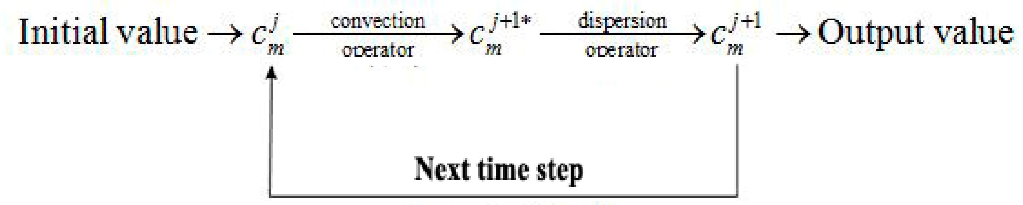
The theoretical model of solute transport in the unsaturated zone under the centrifugal condition is based on the moisture transport model. Equations (19)–(22) represent the four unsaturated solute transport scenarios in this study. The numerical schemes for these equations can be divided into two types. The advection-dispersion Equations (19) and (20) that consider the instantaneous equilibrium adsorption process can be treated as one type. Equations (21) and (22) can be treated as another type, as equation (21) can be considered as a special situation of Equation (22) without reverse reaction (k_b = 0). A method called Operator-Split Method (OSM) has been adopted to numerically discretize the differential equations [48]. Instead of calculating simultaneously, OSM divides the advection-dispersion equation into convection operator and dispersion operator while the transport equation into a transport operator and reactive operator.

Numerical discretization of Equation (20).

First, the equation is divided into convection operator and dispersion operator:

$$\frac{\partial c_m}{\partial t_m}=\underset{\mathit{convection}\mathit{operator}}{\underbrace{-\left(\frac{v_m}{R_m}\right)\frac{\partial c_m}{\partial r}}}+\underset{\mathit{dispersion}\mathit{operator}}{\underbrace{\left(\frac{D_m}{R_m}\right)\frac{{\partial }^2{c}_m}{\partial r^2}}}$$

For the convection part, the forward explicit finite difference method is applied:

$$\frac{c_{m,i}^{j+1^{*}}-c_{m,i}^j}{\Delta t_m}=-\left(\frac{v_{m,i}^j}{R_{m,i}^j}\right)\left(\frac{c_{m,i+1}^j-c_{m,i}^j}{\Delta r}\right)$$

(23)

where $c_{m,i}^{j+1*}$ is the updated concentration, which connects both split operators; $v_{m,i}^j$ and $R_{m,i}^j$ are the seepage velocity and retardation coefficient, respectively, of the previous time step at this point that are calculated by the moisture transport model. Then, put $c_{m,i}^{j+1*}$ into the dispersion operator to carry out the implicit difference discretization:

$$\frac{c_{m,i}^{j+1}-c_{m,i}^{j+1^{*}}}{\Delta t_m}=\left(\frac{D_m}{R_{m,i}^j}\right)\left(\frac{c_{m,i-1}^{j+1}-2c_{m,i}^{j+1}+c_{m,i+1}^j}{\Delta r^2}\right)$$

(24)

Further, we can get:

$$c_{m,i+1}^{j+1}-\left(\frac{1}{{\sigma }_{m,i}^j}+2\right)c_{m,i}^{j+1}+c_{m,i-1}^{j+1}=-\frac{c_{m,i}^{j+1^{*}}}{{\sigma }_{m,i}^j}\mathrm{where}{\sigma }_{m,i}^j=\frac{D_m\Delta t_m}{R_{m,i}^j\Delta r^2}$$

(25)

Apply this equation to all nodes in order to get an equation set. Like the moisture transport model, this equation set can be solved using the chasing and driving method. The computational pipeline of OSM is shown in Figure 2.

Numerical discretization of Equation (22).

First, the equation is divided into transport operator and reactive operator:

$$\{\begin{array}{l}\frac{\partial c_{AM}}{\partial t_m}=\underset{transportoperator}{\underbrace{-(\frac{v_m}{R_{Am}})\frac{\partial c_{AM}}{\partial r}+(\frac{D_{Am}}{R_{Am}})\frac{{\partial }^2{c}_{AM}}{\partial r^2}}}+\underset{reactiveoperator}{\underbrace{k_b\frac{R_{Bm}}{R_{Am}}{c}_{BM}-k_a{c}_{AM}}}\\ \frac{\partial c_{BM}}{\partial t_m}=\underset{transportoperator}{\underbrace{-(\frac{v_m}{R_{Bm}})\frac{\partial c_{BM}}{\partial r}+(\frac{D_{Bm}}{R_{Bm}})\frac{{\partial }^2{c}_{BM}}{\partial r^2}}}+\underset{reactiveoperator}{\underbrace{k_a\frac{R_{Am}}{R_{Bm}}{c}_{BM}-k_b{c}_{BM}}}\end{array}$$

Here, the transport part will be dispersed with implicit finite difference method:

$$\{\begin{array}{l}\left(-{\epsilon }_{Am,i}^j-{\sigma }_{Am,i}^j\right)c_{Am,i-1}^{j+1}{}^{*}+\left(1+2{\sigma }_{Am,i}^j\right)c_{Am,i}^{j+1}{}^{*}+\left({\epsilon }_{Am,i}^j-{\sigma }_{Am,i}^j\right)c_{Am,i+1}^{j+1}{}^{*}=c_{Am,i}^j\\ \left(-{\epsilon }_{Bm,i}^j-{\sigma }_{Bm,i}^j\right)c_{Bm,i-1}^{j+1}{}^{*}+\left(1+2{\sigma }_{Bm,i}^j\right)c_{Bm,i}^{j+1}{}^{*}+\left({\epsilon }_{Bm,i}^j-{\sigma }_{Bm,i}^j\right)c_{Bm,i+1}^{j+1}{}^{*}=c_{Bm,i}^j\end{array}$$

(26)

where ${\sigma }_{Am,i}^j=\frac{D_{Am}\Delta t_m}{R_{Am,i}^j\Delta r^2},{\sigma }_{Bm,i}^j=\frac{D_{Bm}\Delta t_m}{R_{Bm,i}^j\Delta r^2},{\epsilon }_{Am,i}^j=\frac{v_m\Delta t_m}{2R_{Am,i}^j\Delta r},{\epsilon }_{Bm,i}^j=\frac{v_m\Delta t_m}{2R_{Bm,i}^j\Delta r}$

Put the calculation results of $c_{Am,i}^{j+1}{}^{*}$ and $c_{Bm,i}^{j+1}{}^{*}$ into the reactive operator and use the fourth-order Runge Kutta integral algorithm to solve the half part of the equation. If we write $f_A^{RK4}\left(t_m{,c}_{Am}{,c}_{Bm}\right)=\frac{\partial C_{Am}}{\partial t_m}$ and $f_B^{RK4}\left(t_m{,c}_{Am}{,c}_{Bm}\right)=\frac{\partial C_{Bm}}{\partial t_m}$, then we can get:

$$\{\begin{array}{l}{c}_{Am,i}^{j+1}=c_{Am,i}^{j+1}{}^{*}+\frac{\left(S_{A1}+2S_{A2}+2S_{A3}+S_{A4}\right)}{6}\Delta t_m\\ c_{Bm,i}^{j+1}=c_{Bm,i}^{j+1}{}^{*}+\frac{\left(S_{B1}+2S_{B2}+2S_{B3}+S_{B4}\right)}{6}\Delta t_m\end{array}$$

(27)

where

$$\{\begin{array}{l}{S}_{A1}=f_A^{RK4}\left(j\Delta t_m,c_{Am,i}^{j+1}{}^{*},c_{Bm,i}^{j+1}{}^{*}\right)\\ S_{A2}=f_A^{RK4}\left(\left(j+0.5\right)\Delta t_m,c_{Am,i}^{j+1}{}^{*}+0.5S_{A1}\Delta t_m,c_{Bm,i}^{j+1}{}^{*}+0.5S_{B1}\Delta t_m\right)\\ S_{A3}=f_A^{RK4}\left(\left(j+0.5\right)\Delta t_m,c_{Am,i}^{j+1}{}^{*}+0.5S_{A2}\Delta t_m,c_{Bm,i}^{j+1}{}^{*}+0.5S_{B2}\Delta t_m\right)\\ S_{A4}=f_A^{RK4}\left(\left(j+1\right)\Delta t_m,c_{Am,i}^{j+1}{}^{*}+S_{A3}\Delta t_m,c_{Bm,i}^{j+1}{}^{*}+S_{B3}\Delta t_m\right)\\ S_{B1}=f_B^{RK4}\left(j\Delta t_m,c_{Am,i}^{j+1}{}^{*},c_{Bm,i}^{j+1}{}^{*}\right)\\ S_{B2}=f_B^{RK4}\left(\left(j+0.5\right)\Delta t_m,c_{Am,i}^{j+1}{}^{*}+0.5S_{A1}\Delta t_m,c_{Bm,i}^{j+1}{}^{*}+0.5S_{B1}\Delta t_m\right)\\ S_{B3}=f_B^{RK4}\left(\left(j+0.5\right)\Delta t_m,c_{Am,i}^{j+1}{}^{*}+0.5S_{A2}\Delta t_m,c_{Bm,i}^{j+1}{}^{*}+0.5S_{B2}\Delta t_m\right)\\ S_{B4}=f_B^{RK4}\left(\left(j+1\right)\Delta t_m,c_{Am,i}^{j+1}{}^{*}+S_{A3}\Delta t_m,c_{Bm,i}^{j+1}{}^{*}+S_{B3}\Delta t_m\right)\end{array}$$

(28)

3.2.2. Initial and Boundary Conditions

As the object of this study is the groundwater pollution, it is assumed that the soil of the centrifugal model and the prototype do not contain solute at the initial time:

$$c_m\left(r_t\le r\le r_b,t_m=0\right)=0$$

(29)

The solute pollution in groundwater in a real situation is usually this type: the garbage containing pollutants spreads on the surface, and then in a rainy day, the solute of the garbage leaches out and infiltrates into the ground along with the rain to contaminate the soil and groundwater. Therefore, the boundary conditions are: the one-dimensional soil column top provides a temporary solution supply, the concentration of solute A remains constant first and then changes into 0 g/m³, the upper hydraulic boundary changes from the fixed matrix suction of 0 Kpa to the flow flux of 0 m/s; the bottom of the model is a free flow boundary, the matrix suction is fixed to be 0 Kpa, and it is treated as constant diffusion flux boundary condition during the transport process. The boundary conditions can be expressed as follows:

$$\{\begin{array}{l}{c}_m\left(r_t,t_m\le t_{pulse}\right)=c^0\\ c_m\left(r_t,t_{pulse}\le t_m\right)=0\\ \frac{{\partial }^2{c}_m}{\partial r^2}\left(r_b,t_m\right)=0\end{array}$$

(30)

where c⁰ is the initial concentration, t_pulse is the rainfall event duration. The third formula of equation (30) can be expressed in the format of Equation (25):

$$c_{m,i-1}^{j+1}-2c_{m,i}^{j+1}+c_{m,i+1}^{j+1}=0$$

(31)

3.3. Validity Assessment of Centrifugal Modeling

3.3.1. Nonreactive Solute

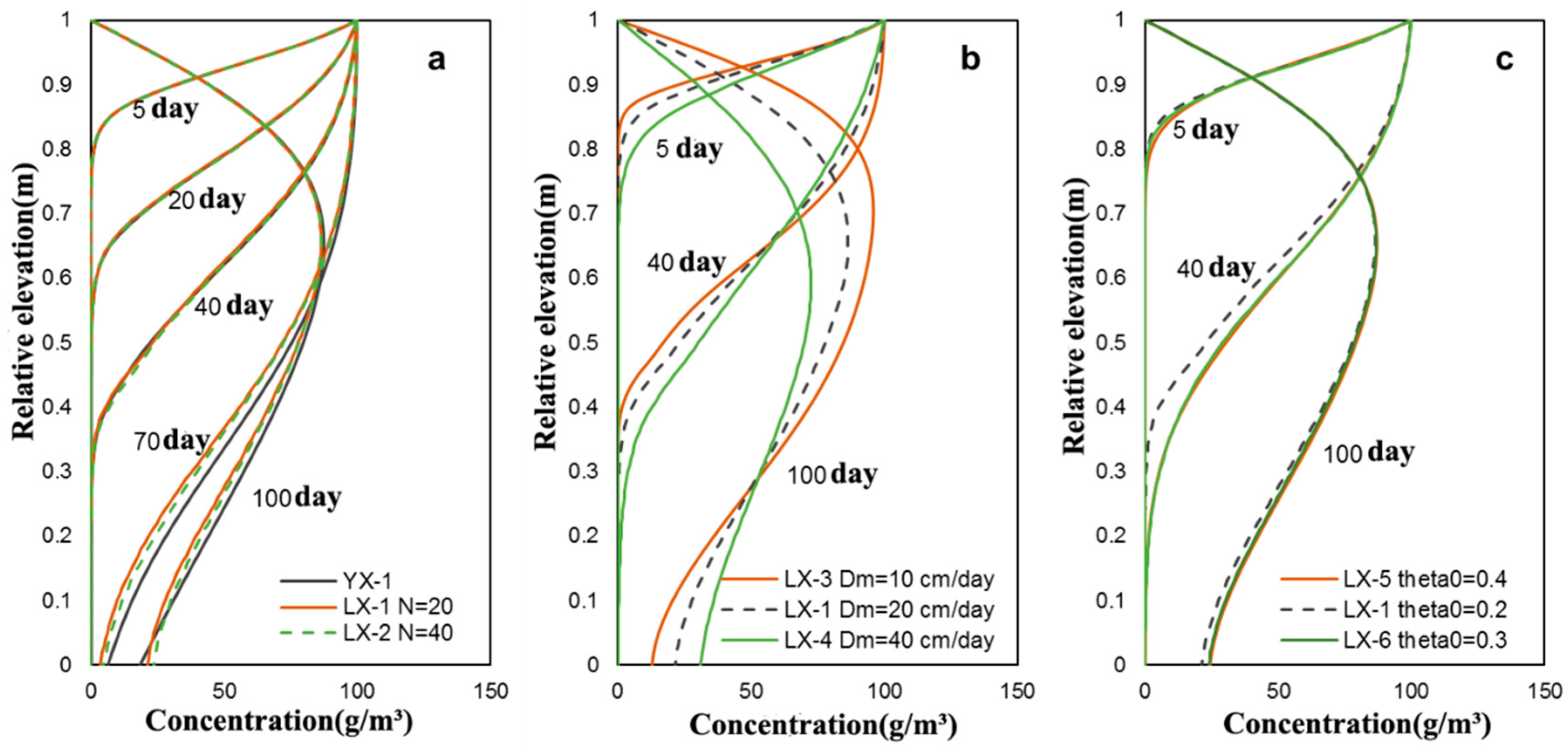
As there is neither adsorption (K_d = 0 m³/g) nor chemical reactions in the transport of nonreactive solute, the centrifugal model can correctly reflect the behavior of the prototype from the view of centrifugal similar theory. Therefore, it is widely used in the study of the solute transport mechanism in the unsaturated zone [22,26]. The fixed parameters and related values are: θ_r = 0.034, θ_s = 0.46, n _v= 1.37, α= 0.016 cm⁻¹, K_s = 1 × 10⁻⁷ m/s, r_b = 2 m, the discretization nodes number n = 101, the concentration of solute A is 100 g/m³. Hereof, θ_r is residual moisture content, θ_s is saturated moisture content, n_v and α are the parameters of the Van Genuchten model that are used to describe the Soil Water Retention Curve (SWRC) [47,49], and K_s is the saturated hydraulic conductivity of the soil. The simulation length of the prototype is 100 days, the rainfall event duration is 75 days, and the unsaturated zone thickness of the prototype is 2 m. The values of other variable parameters are listed in

Table 3. The values of the numerical simulation of the nonreactive substance

Simulation Number	D (cm/day)	θ0	N (g)	L (m)	Simulation Time (h)	Δt (h)
LX-1	20	0.2	20	0.1	6	0.01
LX-2	20	0.2	40	0.05	1.5	0.0025
YX-1	20	0.2	—	2	2400	4
LX-3	10	0.2	20	0.1	6	0.01
LX-4	40	0.2	20	0.1	6	0.01
LX-5	20	0.4	20	0.1	6	0.01
LX-6	20	0.3	20	0.1	6	0.01

Note: ‘YX’ represents the prototype, ‘LX’ represents the centrifugal model, D is hydrodynamic dispersion coefficient, θ₀ is the initial moisture content, N is the gravity level, L is the height of the centrifugal model, and Δt is time step. The meanings are similar hereinafter.

, and the simulation results are shown in Figure 3.

From Figure 3a, it can be seen that the nonreactive solute transport in the unsaturated zone under the centrifugal condition is basically identical with the transport under the prototype condition, but there is a certain deviation near the bottom, where the transport of the model is slightly lagging behind the transport of the prototype. As there is a radial distribution of the centrifugal acceleration, the similarity ratio of the part from 2/3 height to the bottom is underestimated, and the space size is reduced, causing a certain artificial lag in the water and solute transports. In addition, the bias at the bottom is smaller under the condition of N = 40 than that of N = 20, which indicates that it is helpful to reduce this phenomenon by using a bigger N for the same equipment. Figure 3b shows that the bigger the molecular diffusion coefficient is, the larger the solute pollution range is, but the peak concentration would become smaller. This is because the bigger the molecular diffusion coefficient is, the stronger the ‘chipping peak off and filling valley up’ capacity on the concentration profile curve is. Figure 3c infers that the lower the initial moisture content is, the greater the impediment of the soil to the solute transport is. Based on this rule, the dry areas with low soil moisture content are generally chosen as nuclear waste landfills.

Generally speaking, the centrifugal experiment modeling technology can well reflect the nonreactive solute transport behavior in the prototype. There are two schemes to reduce the error due to the centrifugal acceleration distribution: strictly calculate the gravity levels of different parts to correctly handle the scaling of the model size to avoid such error or use a larger N to reduce such error.

3.3.2. Adsorption Solute

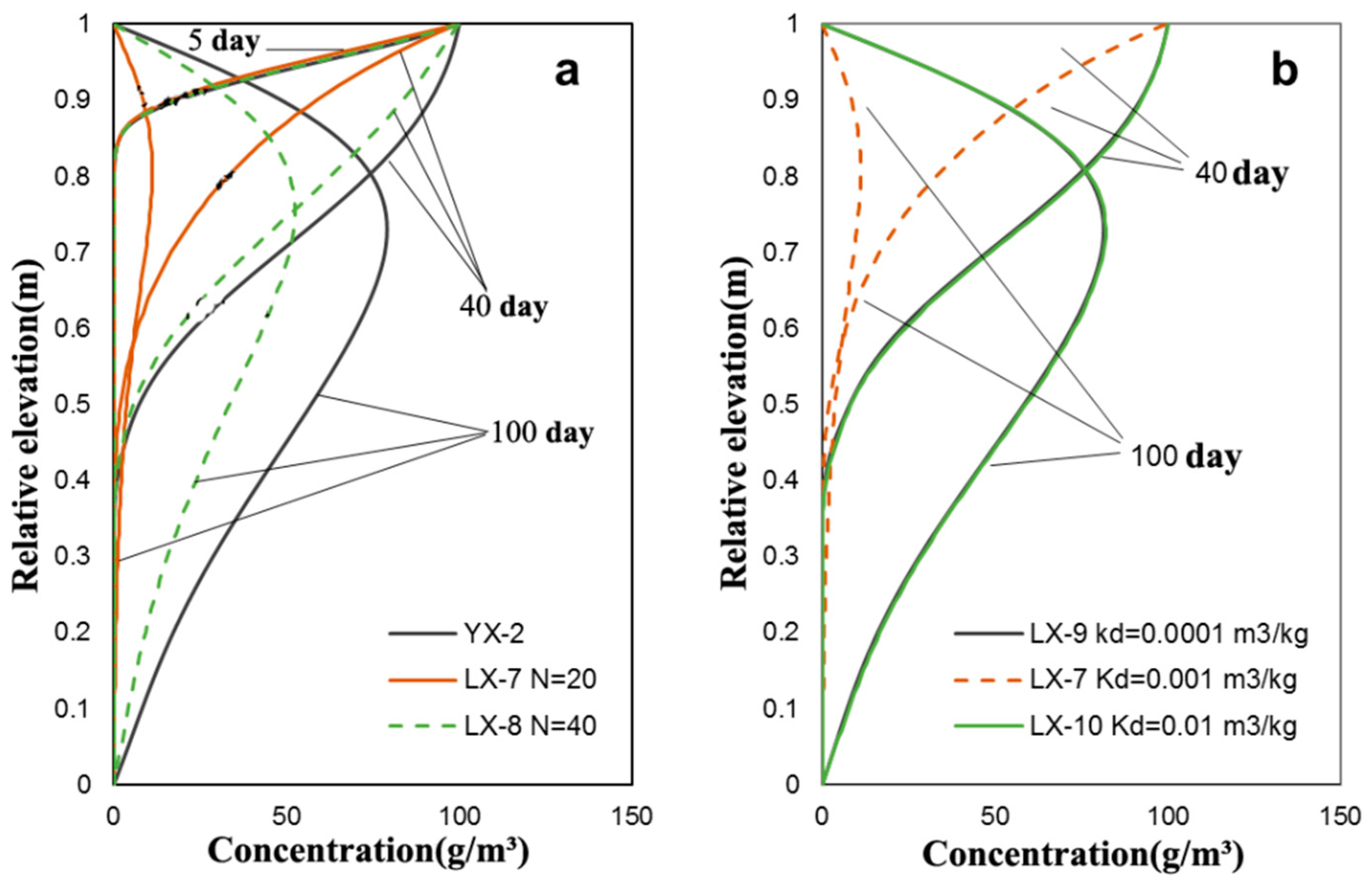
The fixed parameters and related values are: θ_r = 0.034, θ_s = 0.46, n_v = 1.37, α = 0.016 cm⁻¹, K_s = 1 × 10⁻⁷ m/s, r_b = 2m, D_m = 20 cm/day, ρ_b = 1.7 g/m³, the discretization nodes number n = 101, the initial moisture content is 0.2 (uniform distribution), the concentration of solute A is 100 g/m³. The simulation length of the prototype is 100 days, the rainfall event duration is 75 days, and the unsaturated zone thickness of the prototype is 2 m. The values of other variable parameters are listed in

Table 4. The values of the numerical simulation of the adsorption substance

Simulation Number	N (g)	L (m)	Simulation Time (h)	Δt (h)	Kd (m3/kg)
YX-2	—	2	2400	4	0.001
LX-7	20	0.1	6	0.01	0.001
LX-8	40	0.05	1.5	0.0025	0.001
LX-9	20	0.1	6	0.01	0.0001
LX-10	20	0.1	6	0.01	0.01

Note: ‘YX’ represents the prototype, ‘LX’ represents the centrifugal model and K_d is adsorption coefficient.

, and the simulation results are shown in Figure 4.

Figure 4a shows that the results of the centrifugal experiment simulation coincide with that of the prototype, which indicates that it is feasible to apply the centrifugal technology to the instantaneous equilibrium adsorption solute transport in the unsaturated zone. Compared with Figure 4a, the existence of adsorption will very clearly block the solute diffusion, which has positive significance to the pollution range control. However, the cost of this significance is that the solute residues will be in the soil for a long time, which has an impact on the agriculture and the crops. Figure 4b shows the bigger the distribution coefficient is, the stronger the hysteresis effect of soil on the solute is. This will result in slower solute transport, and the pollution range will be more concentrated.

It is a pity that only equilibrium adsorption is discussed in this study, while the non-equilibrium adsorption is more common in the actual situation. At present the dual-domain model, where the pore water is divided into mobile water and immobile water, is commonly used to describe the non-equilibrium adsorption transport. The solute transport mainly occurs in the mobile water zone, while the non-equilibrium exchange of solute occurs between the mobile water zone and immobile water zone. There are pervasive studies on the dual-domain model of the centrifugal experiment modeling, such as Li et al. [50]. The results indicated that it is also feasible to apply the centrifugal experiment modeling in the non-equilibrium adsorption solute transport in the unsaturated zone.

3.3.3. Radionuclide Solute

The fixed parameters and related values are: θ_r = 0.034, θ_s = 0.46, n_v = 1.37, α = 0.016 cm⁻¹, K_s = 1 × 10⁻⁷ m/s, r_b = 2 m, D_m = 20 cm/day, ρ_b = 1.7 g/m³, K_d = 0.0001 m³·kg, the number of discretization nodes n = 101, the initial moisture content is 0.2 (uniform distribution), the concentration of solute A is 100 g·m³. The simulation length of the prototype is 100 days, the rainfall event duration is 75 days, and the unsaturated zone thickness of the prototype is 2 m. The values of other variable parameters are listed in

Table 5. The values of the numerical simulation of the adsorption substance

Simulation Number	N (g)	L (m)	Simulation Time (h)	Δt (h)	λ (s−1)	Half-Life Period (Day)
YXR-1	—	2	2400	4	5 × 10−7	16.0
LXR-1	20	0.1	6	0.01	5 × 10−7	16.0
LXR-2	40	0.05	1.5	0.0025	5 × 10−7	16.0
YXR-2	—	2	2400	4	1 × 10−7	80.2
LXR-3	20	0.1	6	0.01	1 × 10−7	80.2
LXR-4	40	0.05	1.5	0.0025	1 × 10−7	80.2
YXR-3	—	2	2400	4	1 × 10−8	802.3
LXR-5	20	0.1	6	0.01	1 × 10−8	802.3
LXR-6	40	0.05	1.5	0.0025	1 × 10−8	802.3

Note: ‘YXR’ represents the prototype with radionuclide solute, ‘LXR’ represents the centrifugal model with radionuclide solute, and λ is the nuclide decay coefficient.

, and the simulation results are shown in Figure 5.

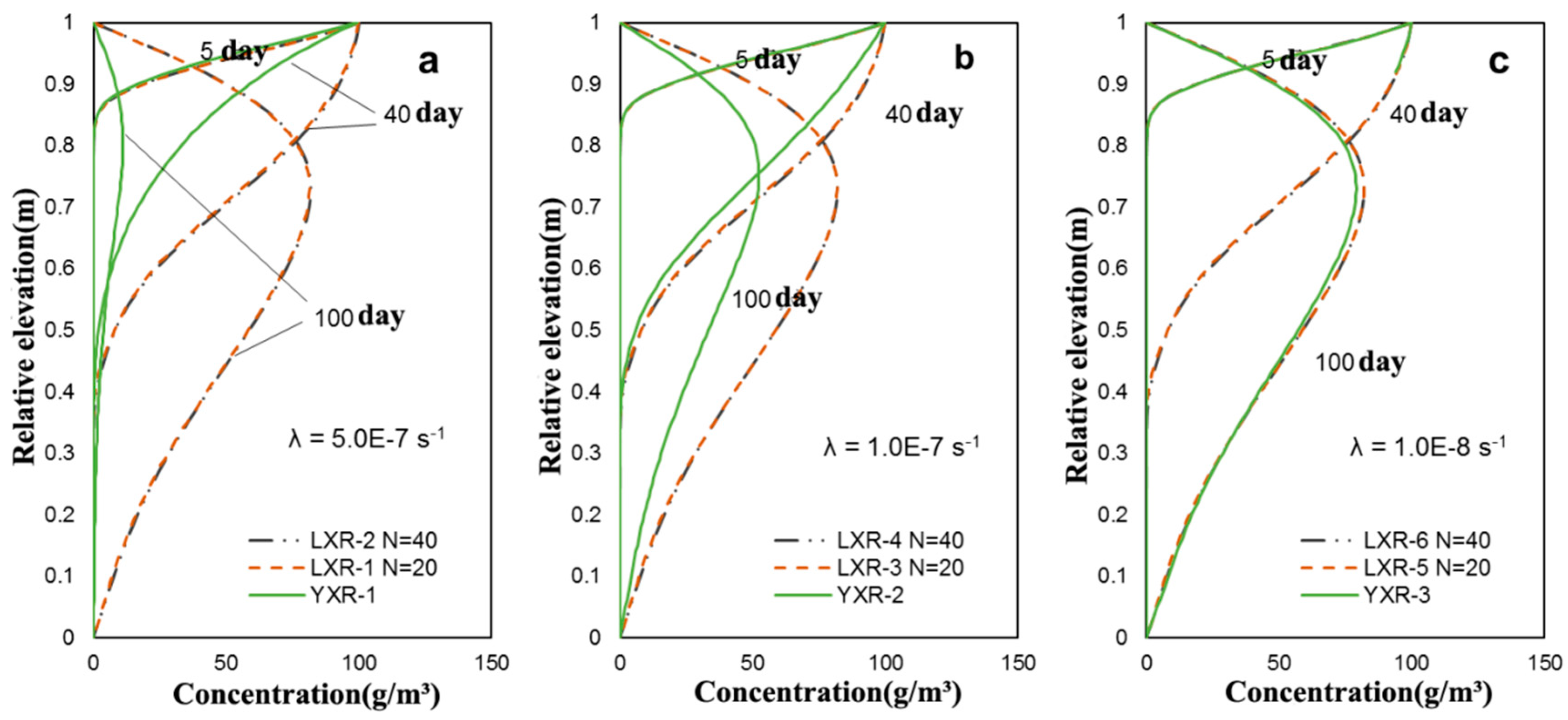
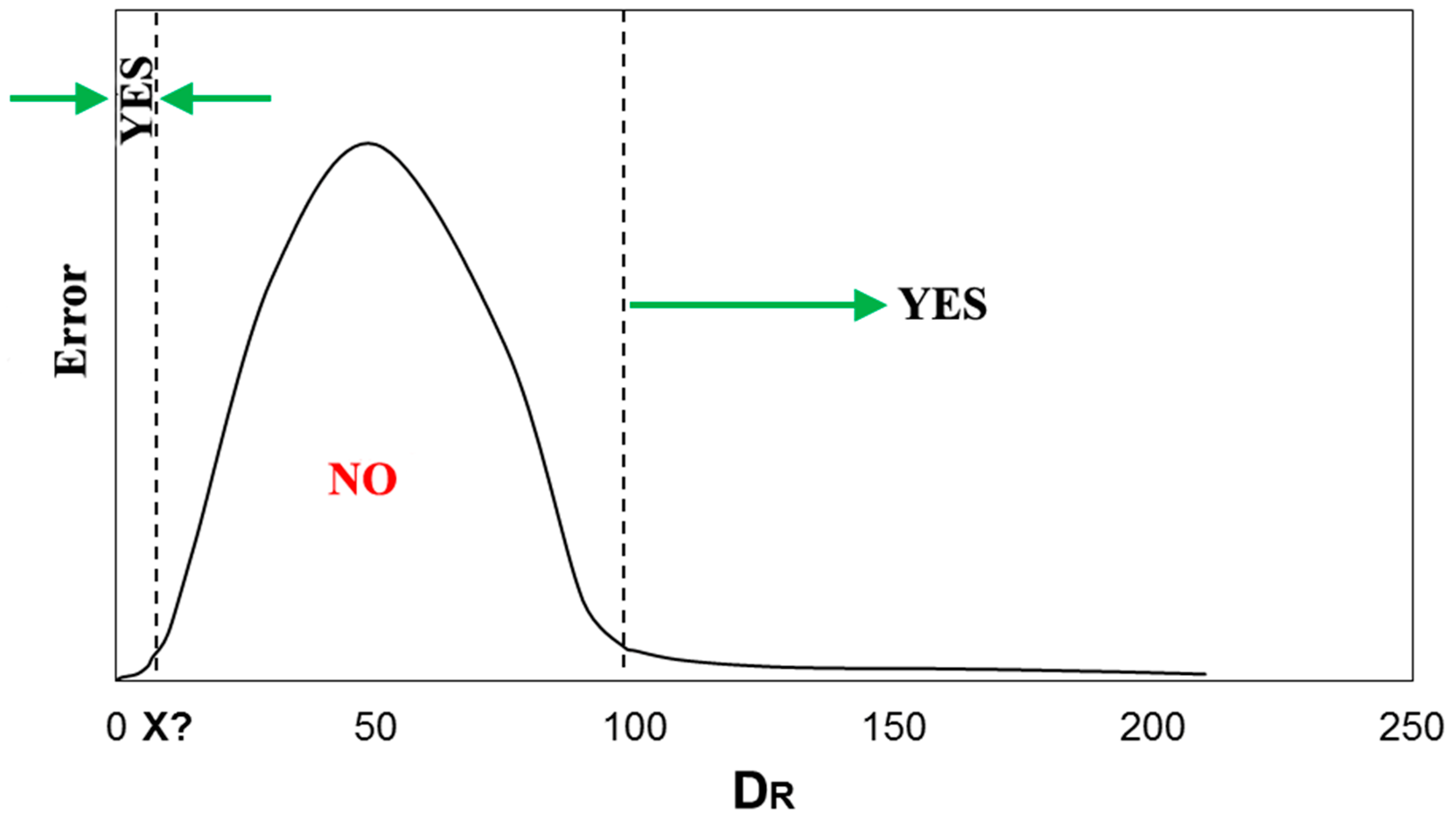
Figure 5 shows that the decay coefficient λ is very important to the question of whether the centrifugal model can successfully predict the radionuclide transport behavior of the prototype. The chemical process cannot be accelerated in the centrifugal model, while the simulation time of the centrifugal model is only 1/N² of the prototype, causing the chemical process of the prototype not sufficient as one of the centrifugal model. The solute’s ability to transport and the concentration in the pollution areas tend to be overestimated by the centrifugal model under this situation. Figure 5c presents that the centrifugal experiment modeling can accurately predict the radioactive nuclide transport if the nuclear substance’s half-life period is much larger than the simulation time of the prototype (802 days is much larger than 100 days). At this time, the radioactive nuclide can be treated as a nonreactive solute. The centrifugal experiment modeling is also applicable if the non-equilibrium process is very rapid. Cooke and Mitchell [24] have proposed to use the chemical effect number π₉ (Table 2) to measure whether the centrifugal experiment modeling is suitable for the transport process with chemical reaction. The Damoner number D_R proposed by Appelo and Postma [27] is similar to π₉. Appelo and Postma [27] believed that the centrifugal experiment modeling could correctly reflect the transport process of the prototype if D_R is large than 100 (the chemical reaction is very rapid). According to the results, it is believable that if D_R is small enough, the centrifugal experiment modeling error can be controlled within the acceptable range, and then the centrifugal experiment modeling is also applicable for the reactive solute transport (Figure 6). It is of great significance for the centrifugal technology promotion and the related theories development to determine the lower limit value X of D_R. A certain criteria and actual experiment are needed to verify this value. In addition, the comparison of Figure 4a and Figure 5a indicates that the decay process existence is beneficial to the natural elimination of nuclear pollution in the soil.

3.3.4. Reactive Solute

A more complex transport process of reactive solute A with product solute B in the unsaturated zone is further studied and understood in this section. The fixed parameters and related values are: θ_r = 0.034, θ_s = 0.46, n_v = 1.37, α = 0.016 cm⁻¹, K_s = 1 × 10⁻⁷ m/s, r_b = 2 m, D_Am = D_Bm = 20 cm/day, ρ_b = 1.7 g/m, K_Ad = K_Bd = 0.0001 m³/kg, the number of discretization nodes n = 101, the initial moisture content is 0.2 (uniform distribution), the concentration of solute A is 100 g/m³. The simulation length of the prototype is 100 days, the rainfall event duration is 75 days, and the unsaturated zone thickness of the prototype is 2 m. The values of other variable parameters are listed in

Table 6. The values of the numerical simulation of the reactive substance

Simulation Number	N (g)	L (m)	Simulation Time (h)	Δt (h)	ka (s−1)	kb (s−1)
YXF-1	—	2	2400	4	1 × 10−8	1 × 10−8
YXF-2	—	2	2400	4	1 × 10−6	1 × 10−5
LXF-1	20	0.1	6	0.01	1 × 10−8	1 × 10−8
LXF-2	40	0.05	1.5	0.0025	1 × 10−8	1 × 10−8
LXF-3	20	0.1	6	0.01	1 × 10−6	1 × 10−5
LXF-4	40	0.05	1.5	0.0025	1 × 10−6	1 × 10−5

Note: ‘YXF’ represents the prototype with reactive solute, ‘LXF’ represents the centrifugal model with the reactive solute, k_a and k_b are reaction rate constants of A and B, respectively.

, and the simulation results are shown in Figure 7.

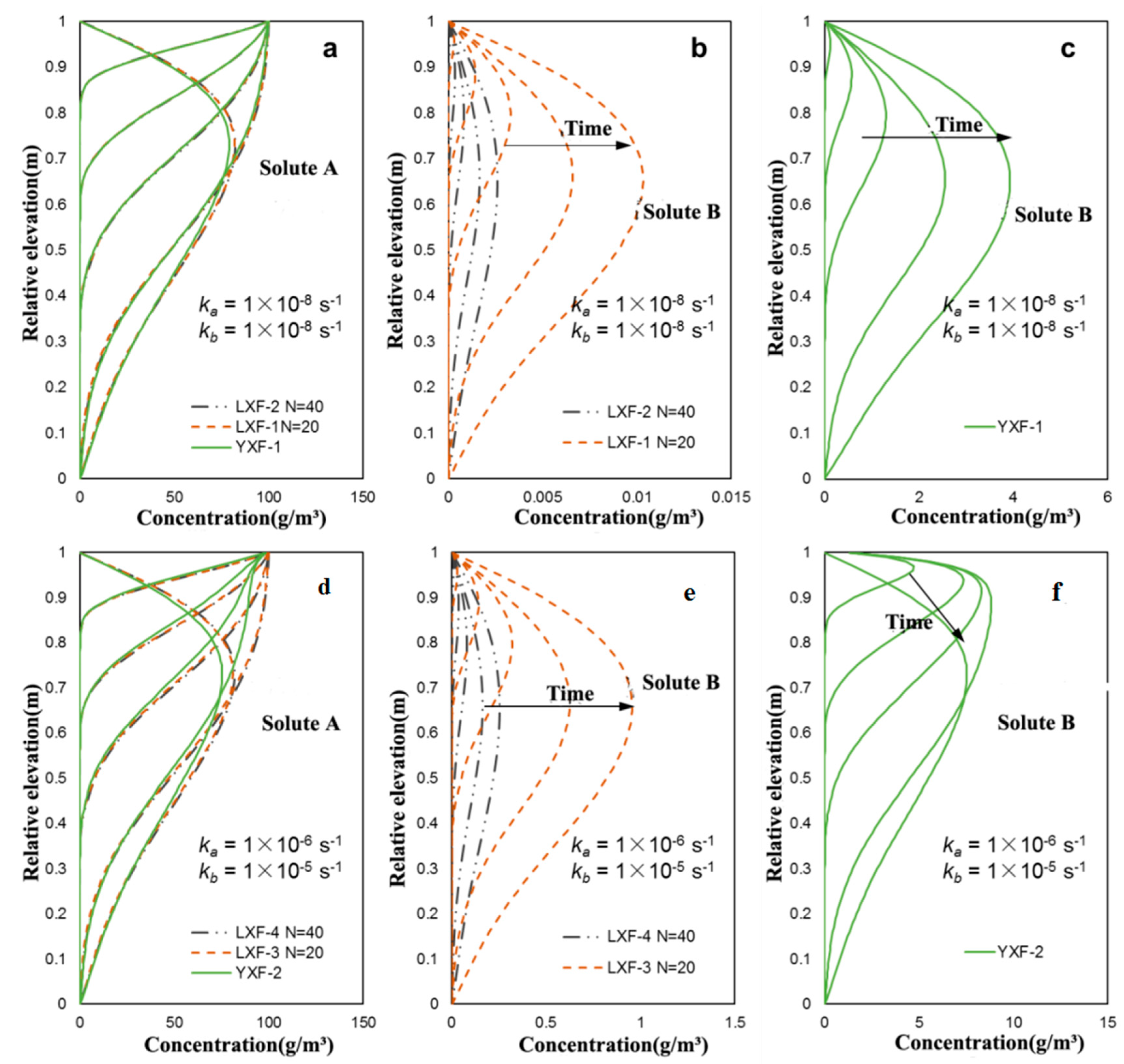
Figure 7a,d present that the presence of chemical reaction can make the centrifugal experiment modeling results deviate from the prototype. If the reaction is slow, the centrifugal experiment modeling of solute A can be well matched with the prototype; while if the reaction is very rapid, the error will be very large, tending to overestimate the ability of solute A of diffusion transport and the concentration of solute A in the pollution area. By further comparing Figure 7b,c as well as Figure 7e,f, it was found that the differences of product solute B in the centrifugal model and the prototype are very large. The concentration prediction error can be up to two orders of magnitude. By the careful examination of Figure 7d and by comparing Figure 7e,f, it was found that the concentration distribution of solute A near the top region of the soil in the prototype has obvious characteristics of steep fall, while the secondary solute B is concentrated and distributed in the top region. However, these characteristics cannot be reflected in the centrifugal model, which indicates that the centrifugal technology can hardly catch the details of the transport process if this technology is applied in solute transport in the unsaturated zone with rapid chemical reaction.

The centrifugal experiment modeling technology is feasible for the transport process of solute A with relatively slow chemical reaction. If the reaction is very rapid, the error in the centrifugal simulation is very large, and the centrifugal technology cannot catch the details in the transport processes. In addition, the concentration prediction error of product solute B using the centrifugal technology can be up to two orders of magnitude compared with the prototype results. This indicates that the centrifugal technology is a loser in the prediction of product solute B. If the product solute B is also an important object of the problem, the centrifugal technology is not worthy of recommendation. On the other hand, if the product solute B is not so important that it can be ignored, the centrifugal experiment modeling technology is feasible under the appropriate condition (not rapid reaction process).

4. Discussion and Conclusions

4.1. Discussion

Unlike the moisture transport, the solute transport in the unsaturated zone has a close relationship with the solute substance itself and the physical and chemical processes the solute is involved in, which results in the complexity of the solute transport modeling. With the help of the gravity acceleration, the centrifugal experiment modeling can speed up the processes of solute transport and then make it possible to carry out numerous modeling of the solute transport in a short period. However, this study focused on solute contaminants rather than organic contaminants. The physical and chemical processes considered in this study are not all-inclusive. There are much more organic contaminants and processes that should be considered in the solute transport in the unsaturated zone, which can be of further research interests of the scientists worldwide.

The other threshold value of the Damoner number (X) is an important and interesting value that is worth further study. Previous studies have determined one threshold value of D_R (100), over which the centrifugal experiment modeling is feasible. That is, if the reaction process is rapid enough, the centrifugal technology can be applied in the solute transport with chemical reaction process. The results in this study revealed that if the process is slow enough, the centrifugal technology is also feasible. However, we did not determine the value of X in this study. This aspect can be improved in future studies. It is of great significance for the centrifugal technology promotion and the related theories development to determine the X value of Damoner number. Certain criteria and actual experiment are needed to verify this lower limit value of Damoner number.

4.2. Conclusions

This study has assessed the application feasibility of centrifugal experiment modeling to solute transport in the unsaturated zone. By comparing the centrifugal model and the prototype using the same numerical model under different solute substances, the feasibility of centrifugal technology under different conditions has been validated.

The centrifugal experiment modeling, which can correctly reflect the solute transport of a nonreactive substance in the prototype, can be applied to such kind of solute transport. However, the radial distribution of centrifugal acceleration makes the solute transport, near the bottom area in the centrifugal model, slightly lags behind the prototype. Using a larger gravity level (N) can make the acceleration distribution more uniform, and hence reduce the error existing in the centrifugal model.

The molecular diffusion coefficient and initial soil moisture content have effects on solute transport. The bigger the molecular diffusion coefficient is, the stronger the ‘chipping peak off and filling valley up’ capacity on the concentration profile curve is. This leads to a more uniform solute distribution, a larger solute pollution range, and a smaller peak concentration. The lower the initial soil moisture content is, the slower the solute transport spread is, which can be used in the pollution spreading control.

The centrifugal experiment modeling is suitable for solute transport with the instantaneous equilibrium adsorption. The existence of adsorption and desorption has a significant effect on solute transport. The greater the distribution coefficient is, the more obvious the soil’s hysteresis effect on the solute is, which has a positive significance for the pollution range control.

For the radioactive nuclide, as the reaction process is not sufficient as the prototype, the centrifugal model overestimates both the ability of solute’s transport and the concentration in the pollution area. But if the radioactive element’s half-life period is much larger than the prototype, the centrifugal experiment modeling technology is feasible for the radioactive nuclide. Usually, the radioactive nuclide can be treated as a nonreactive solute under this circumstance.

For the solute transport with chemical reaction, the predecessors proposed if D_R > 100 and the reaction is very rapid, then the centrifugal experiment modeling is feasible. This study found that if the reaction process is very slow (e.g., half-life period is much larger than the event duration), then the centrifugal experiment modeling is also feasible. Therefore, if 0 < D_R < X (X is unknown), the centrifugal experiment modeling is feasible. The determination of X value is of great significance for the promotion and theoretical development of centrifugal modeling technology.

For the transport of reactive solute A with product B generated in the unsaturated zone, if the reaction process is slow, the transport prediction of solute A by the centrifugal model can well match the prototype. But the prediction error of solute B is very large, with the concentration error up to two orders of magnitude. If solute B is also of focus, then the centrifugal experiment modeling is not worthy of recommendation. If solute B is not so important, then the centrifugal experiment modeling is feasible under the appropriate condition (the reaction process is slow).

References

- Zheng, C.M.; Bennett, G.D. Applied Contaminant Transport Modeling, 2nd ed.; John Wiley & Sons: New York, NY, USA, 2002; pp. 1–15. [Google Scholar]
- Clement, T.P.; Wise, W.R.; Molz, F.J. A physically based, two-dimensional, finite-difference algorithm for modeling variably saturated flow. J. Hydrol. 1994, 161, 71–90. [Google Scholar] [CrossRef]
- Wang, C.; Ruan, X.H.; Zhu, L. Experimental study of contaminant transport in unsaturated soils. J. Hohai Univ. 1996, 24, 7–13, (In Chinese with English abstract). [Google Scholar]
- Marshall, J.D.; Shimada, B.W.; Jaffe, P.R. Effect of temporal variability in infiltration on contaminant transport in the unsaturated zone. J. Contam. Hydrol. 2000, 46, 151–161. [Google Scholar] [CrossRef]
- Pickens, J.F.; Grisak, G.E. Modeling of scale-dependent dispersion in hydrogeologic systems. Water Resour. Res. 1981, 17, 1701–1711. [Google Scholar] [CrossRef]
- Yang, J.Z. Indoor experimental study of the dispersion coefficient. Eng. Surv. 1985, 13, 55–60. (In Chinese) [Google Scholar]
- Cargill, K.W.; Ko, H.Y. Centrifugal modeling of transient water flow. J. Geotech. Eng. 1983, 109, 536–555. [Google Scholar] [CrossRef]
- Arulanandan, K.; Thompson, P.Y.; Kutter, B.L.; Meegoda, N.J.; Muraleetharan, K.K.; Yogachandran, C. Centrifuge modelling of transport processes for pollutants in soils. J. Geotech. Eng. 1988, 114, 185–205. [Google Scholar] [CrossRef]
- Lynch, R.J.; Allersma, H.G.B.; Barker, H.; Bezuijen, A.; Bolton, M.D.; Cartwright, M.; Davies, M.C.R.; Depountis, N.; Esposito, G.; Garnier, J.; et al. Development of sensors, probes and imaging techniques for pollutant monitoring in geo-environmental model tests. Int. J. Phys. Model. Geotech. 2001, 1, 17–27. [Google Scholar] [CrossRef]
- Nimmo, J.R.; Mello, K.A. Centrifugal techniques for measuring saturated hydraulic conductivity. Water Resour. Res. 1991, 27, 1263–1269. [Google Scholar] [CrossRef]
- Singh, D.N.; Kuriyan, S.J. Estimation of hydraulic conductivity of unsaturated soils using a geotechnical centrifuge. Can. Geotech. J. 2002, 39, 684–694. [Google Scholar] [CrossRef]
- Knight, M.; Mitchell, R. Modelling of light non-aqueous phase liquid (LNAPL) releases into unsaturated sand. Can. Geotech. J. 1996, 33, 913–925. [Google Scholar] [CrossRef]
- Gamerdinger, A.P.; Kaplan, D.I.; Wellman, D.M.; Serne, R.J. Two-region flow and decreased sorption of uranium (VI) during transport in Hanford ground water and unsaturated sands. Water Resour. Res. 2001, 37, 3155–3162. [Google Scholar] [CrossRef]
- Zhang, J.; Lo, I.M.C. Centrifuge study of long term transport behavior and fate of copper in soils at various saturation of water, compaction and clay content. Soil Sediment Contam. 2008, 17, 237–255. [Google Scholar] [CrossRef]
- Mckinley, J.D.; Price, B.A.; Lynch, R.J.; Schofield, A.N. Centrifuge modelling of the transport of a pulse of two contaminants through a clay layer. Geotechnique 1998, 48, 421–425. [Google Scholar] [CrossRef]
- Zhang, J.H.; Yan, D. Centrifuge modeling of copper ion migration in unsaturated silty clay. Chin. J. Geotech. Eng. 2004, 26, 792–797, (In Chinese with English abstract). [Google Scholar]
- Esposito, G.; Allersma, H.G.B.; Selvadurai, A.P.S. Centrifuge modeling of LNAPL transport in partially saturated sand. J. Geotech. Geoenviron. Eng. 1999, 125, 1066–1071. [Google Scholar] [CrossRef]
- Hu, L.M.; Hao, R.F.; Yin, K.T.; Lao, M.C. Experimental study of BTEX transport in an unsaturated soil and groundwater system. J. Tsinghua Univ. 2003, 43, 1546–1549, (In Chinese with English abstract). [Google Scholar]
- Menezes, G.B.; Ward, A.; Moo-Young, H.K. Unsaturated flow in anisotropic heterogeneous media: A centrifuge study. Int. J. Hydrol. Sci. Tech. 2011, 1, 147–163. [Google Scholar] [CrossRef]
- Timms, W.; Hendry, M.J.; Muise, J.; Kerrich, R. Coupling centrifuge modeling and laser ablation inductively coupled plasma mass spectrometry to determine contaminant retardation in clays. Environ. Sci. Tech. 2009, 43, 1153–1159. [Google Scholar] [CrossRef]
- Gamerdinger, A.P.; Kaplan, D.I. Application of a continuous-flow centrifugation method for solute transport in disturbed, unsaturated sediments and illustration of mobile-immobile water. Water Resour. Res. 2000, 36, 1747–1755. [Google Scholar] [CrossRef]
- Kumar, P.R. Scaling laws and experimental modelling of contaminant transport mechanism through soils in a geotechnical centrifuge. Geotech. Geol. Eng. 2007, 25, 581–590. [Google Scholar] [CrossRef]
- Taylor, R.N. Geotechnical Centrifuge Technology; CRC Press: London, UK, 2003; pp. 20–34. [Google Scholar]
- Cooke, B.; Mitchell, R.J. Physical modelling of a dissolved contaminant in an unsaturated sand. Can. Geotech. J. 1991, 28, 829–833. [Google Scholar] [CrossRef]
- Nimmo, J.R.; Rubin, J.; Hammermeister, D.P. Unsaturated flow in a centrifugal field: Measurement of hydraulic conductivity and testing of Darcy’s Law. Water Resour. Res. 1987, 23, 124–134. [Google Scholar] [CrossRef]
- Nakajima, H.; Hirooka, A.; Takemura, J.; Mariño, M.A. Centrifuge modeling of one-dimensional subsurface contamination. J. Am. Water Resour. 1998, 34, 1415–1425. [Google Scholar] [CrossRef]
- Appelo, C.A.J.; Postma, D. Geochemistry, Groundwater and Pollution, 2nd ed.; A.A. Balkema: Rotterdam, The Netherlands, 1993; pp. 489–537. [Google Scholar]
- Bucky, P.B. Use of models for the study of mining problems. Am. Inst. Min. Met. Eng. Tech. Publ. 1931, 425, 3–28. [Google Scholar]
- Hu, L.M. The Application of the Geotechnical Centrifugal Model in the Environmental Geotechnical Engineering. In Proceedings of the Academic Annual Conference of China Water Conservancy Society: The Application of Physical Simulation on the Geotechnical Engineering, Suzhou, Jiangsu Province, Shangai, 30 October–1 November 2007; pp. 210–218. (In Chinese). [Google Scholar]
- Lin, M. Progress of geotechnical centrifuge and specialized test device in China. J. Yangtze River Sci. Res. Inst. 2012, 29, 80–84, (In Chinese with English abstract). [Google Scholar]
- Conca, J.L.; Wright, J. Diffusion and flow in gravel, soil, and whole rock. Appl. Hydrogeol. 1992, 1, 5–24. [Google Scholar] [CrossRef]
- Singh, D.N.; Gupta, A.K. Modelling hydraulic conductivity in a small centrifuge. Can. Geotech. J. 2000, 37, 1150–1155. [Google Scholar] [CrossRef]
- McCartney, J.S.; Zornberg, J.G. Centrifuge permeameter for unsaturated soils. II: Measurement of the hydraulic characteristics of an unsaturated clay. J. Geotech. Geoenviron. Eng. 2010, 136, 1064–1076. [Google Scholar] [CrossRef]
- Celorie, J.A.; Vinson, T.S.; Woods, S.L.; Istok, J.D. Modeling solute transport by centrifugation. J. Environ. Eng. 1989, 115, 513–526. [Google Scholar] [CrossRef]
- Zhan, L.T.; Zeng, X.; Li, Y.C.; Zhong, X.L.; Chen, Y.M. Centrifuge modeling for chloridion breaking through Kaolin clay liner with high hydraulic head. J. Yangtze River Sci. Res. Inst. 2012, 29, 83–89, (In Chinese with English abstract). [Google Scholar]
- Levy, L.C.; Culligan, P.J.; Germaine, J.T. Use of the geotechnical centrifuge as a tool to model dense nonaqueous phase liquid migration in fractures. Water Resour. Res. 2002, 38, 31–34. [Google Scholar] [CrossRef]
- Ataie-Ashtiani, B.; Hassanizadehb, S.M.; Oungc, O.; Bezuijenc, F.A.W.A. Numerical modelling of two-phase flow in a geocentrifuge. Environ. Model. Softw. 2003, 18, 231–241. [Google Scholar] [CrossRef]
- Xu, Y.B.; Wei, C.F.; Li, H.; Chen, H. Finite element analysis of coupling seepage and deformation in unsaturated soils. Rock Soil Mech. 2009, 30, 1490–1496, (In Chinese with English abstract). [Google Scholar]
- Basford, J.; Goodings, D.; Torrents, A.; Madabhushi, S. Fate and Transport of Lead Through Soil at 1 g and in the Centrifuge. In Proceedings of the 5th International Conference on Physical Modelling in Geotechnics, St. John’s, NL, Canada, 10–12 July 2002; pp. 379–383. [Google Scholar]
- Zhang, J.H.; Lv, H.; Wang, W.C. Centrifuge modeling of copper ionic migration in unsaturated soils. Rock Soil Mech. 2006, 27, 1885–1890, (In Chinese with English abstract). [Google Scholar]
- Gurumoorthy, C.; Singh, D.N. Diffusion of iodide, cesium and strontium in charnockite rock mass. J. Radioanal. Nucl. Chem. 2005, 262, 639–644. [Google Scholar] [CrossRef]
- Gurumoorthy, C.; Kusakabe, O. Experimental methodology to assess migration of iodide ion through bentonite-sand backfill in a near surface disposal facility. Indian J. Sci. Technol. 2012, 5, 1834–1839. [Google Scholar]
- Hu, L.M.; Lo, I.M.C.; Meegoda, J.N. Centrifuge testing of LNAPL migration and soil vapor extraction for soil remediation. Pract. Period. Hazard. Toxic Radioact. Waste Manag. 2006, 10, 33–40. [Google Scholar] [CrossRef]
- Hellawell, E.; Savvidou, C.; Booker, J. Modelling of contaminated land reclamation. Soils Found. 1994, 34, 71–79. [Google Scholar] [CrossRef]
- Ratnam, S.; Culligan-Hensley, P.; Germaine, J. Modeling the Behavior of LNAPLS Under Hydraulic Flushing. In Proceedings of the Conference on Non-Aqueous Phase Liquids (NAPLs) in Subsurface Environment: Assessment and Remediation, Washington, DC, USA, 10–14 November 1996; pp. 595–606. [Google Scholar]
- Penn, M.; Savvidou, C.; Hellawell, E. Centrifuge Modelling of the Removal of Heavy Metal Pollutants Using Electrokinetics. In Proceedings of the Second International Congress on Environmental Geotechnics, Osaka, Japan, 5–8 November 1996; pp. 1055–1060. [Google Scholar]
- Qin, H.H. Investigation on the feasibility of centrifugal simulation on water migration in vadose zone. J. Yangtze River Sci. Res. Inst. 2019, 36, 13–20, 28, (In Chinese with English abstract). [Google Scholar]
- Tapley, B.; Celledoni, E.; Owren, B.; Andersson, H.I. A novel approach to rigid spheroid models in viscous flows using operator splitting methods. Numer. Algorithms 2019. [Google Scholar] [CrossRef]
- Genuchten, M.T.V. A closed-form equation for predicting the hydraulic conductivity of unsaturated soils. Soil Sci. Soc. Am. J. 1980, 44, 892–898. [Google Scholar] [CrossRef]
- Li, L.; Barry, D.A.; Hensley, P.J.; Bajracharya, K. Nonreactive Chemical Transport in Structured Soil: The Potential for Centrifuge Modelling. In Proceedings of the Conference on Geotechnical Management of Waste and Contamination, Sydney, Australia, 22–23 March 1993; pp. 425–431. [Google Scholar]
Figure 1.
The diagram of the centrifugal experiment modeling: (a) the prototype and (b) the centrifugal model. Where Lp, Lm and vp, vm present the length and the seepage velocity of the prototype and the centrifugal model, respectively; ω is the angular velocity of the centrifuge.
Figure 2.
The computational pipeline of the Operator-Split Method (OSM).
Figure 3.
The feasibility comparison of the centrifugal experiment modeling of the nonreactive solute transport in the unsaturated zone (the time in the figure is the prototype time): (a) comparison of the prototype and the centrifugal model; (b) effects of molecular dispersion coefficient on solute transport; and (c) effects of different initial moisture content on solute transport.
Figure 4.
The feasibility comparison of the centrifugal experiment modeling of the adsorption solute transport in the unsaturated zone (the time in the figure is the prototype time): (a) comparison of the prototype and the centrifugal model; and (b) effects of adsorption coefficient on solute transport.
Figure 5.
The feasibility comparison of the centrifugal experiment modeling of the radionuclide solute transport in the unsaturated zone (the time in the figure is the prototype time) with the λ values of 5×10⁻⁷, 1×10⁻⁷ and 0.1×10⁻⁷ for (a), (b) and (c), respectively.
Figure 6.
The range of Damoner number (DR) that determines whether the centrifugal experiment modeling of the reactive solute is feasible.
Figure 7.
The feasibility comparison of the centrifugal experiment modeling of the reactive solute transport in the unsaturated zone (the time is the prototype time): (a) and (d) compare the effects of different reactive rates on solute A; (b) and (e) compare the effects of different reactive rates on solute B under the centrifugal environment; and (c) and (f) compare the effects of different reactive rates on solute B in the prototype.