Spatial Downscaling of Tropical Rainfall Measuring Mission (TRMM) Annual and Monthly Precipitation Data over the Middle and Lower Reaches of the Yangtze River Basin, China


Abstract
:1. Introduction
2. Data and Methods
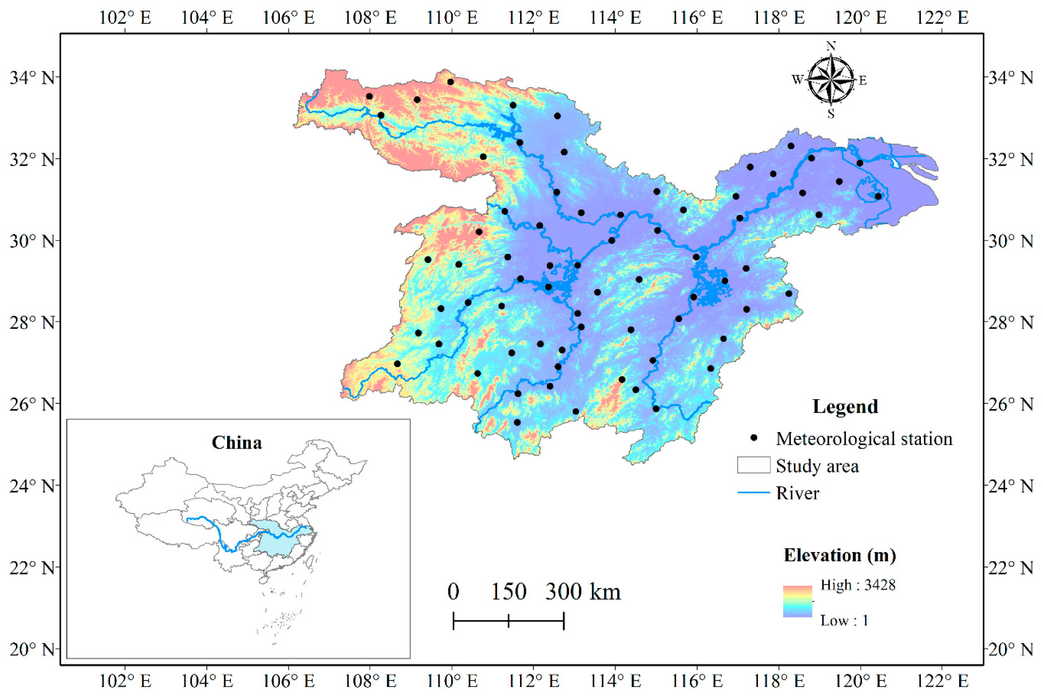
2.1. Study Area
2.2. Data
2.3. Methodology
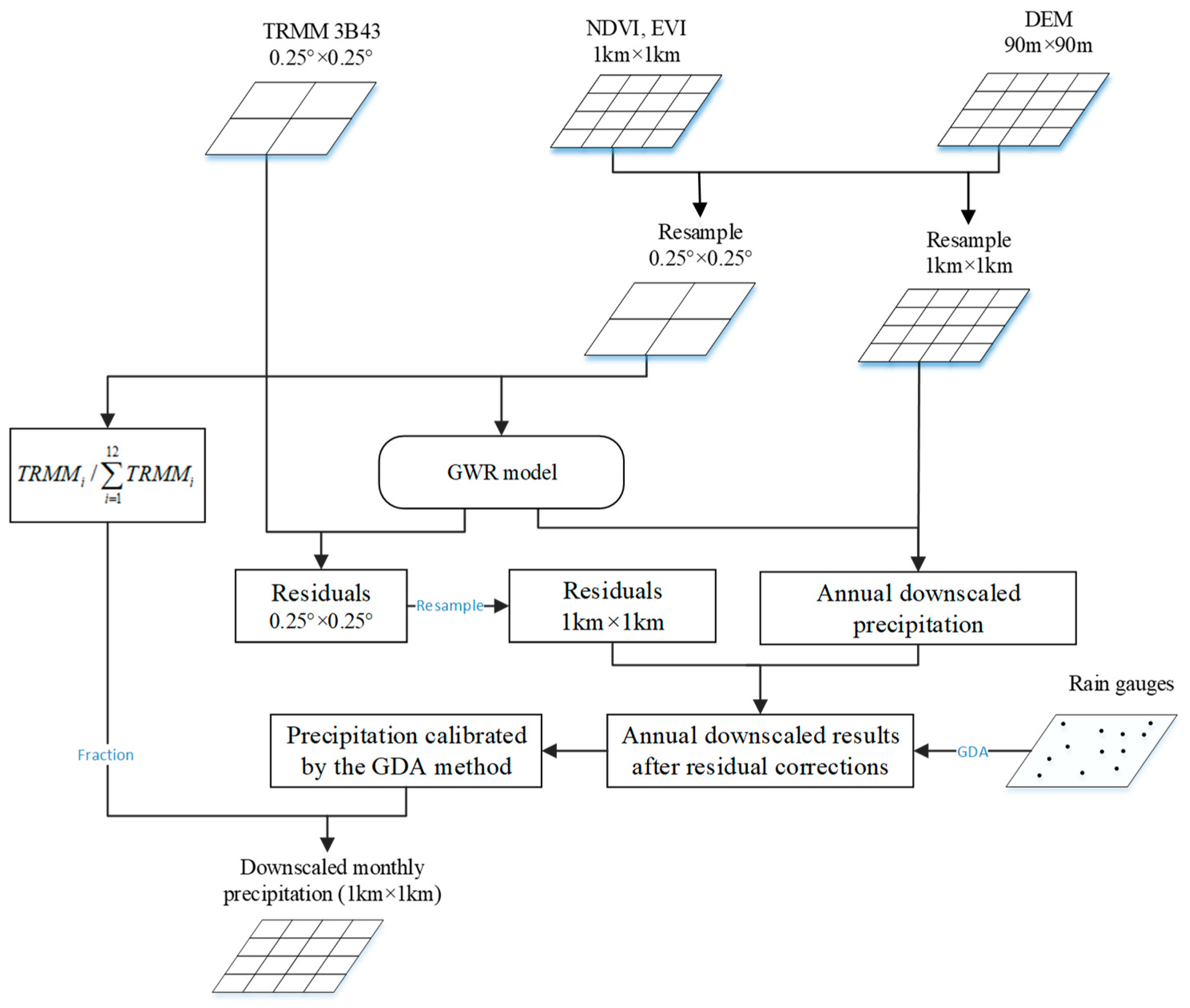
- Monthly TRMM precipitation data during the period 2000–2016 are accumulated to obtain the annual precipitation data, the monthly EVI1km is averaged to obtain the annual EVI1km, and the 1-km resolution EVI and DEM data are resampled to a 0.25° resolution by bilinear interpolation. The model parameters in Equation (1), namely, , and , are obtained at a spatial resolution of 0.25° by using the GWR model;
- The model parameters, namely, , , and , are resampled to 1 km using bilinear interpolation, where , , and represent the model parameters at a 1-km resolution;
- The annual precipitation is estimated at a 1-km resolution by using the 1-km model parameters obtained in the previous step with the following equation:
- The residual at a 0.25° resolution is interpolated into a resolution of 1 km using ordinary kriging [43], the result of which is expressed as . Then, the downscaled precipitation is obtained by adding the 1-km precipitation estimated in the previous step to the residual , and the result can be expressed as follows:
- The geographical differential analysis (GDA) method proposed by Cheema et al. [44], based on residual merging algorithms for multisource data, is used to reduce the difference between the observation data and the downscaled precipitation data [45]. The difference between the downscaled precipitation data and the corresponding meteorological observation data is calculated using Equation (4), after which is interpolated into a 1-km resolution as using ordinary kriging. Then, is subtracted from the downscaled data to obtain the downscaled and calibrated precipitation data :
- The fraction is obtained by calculating the ratio of the monthly TRMM 3B43 precipitation data to the annual precipitation as follows [46]:where TRMMi represents the original TRMM precipitation at a 0.25° resolution in the ith month of the year, and the denominator is the corresponding annual precipitation;
- Ordinary kriging interpolation is employed to interpolate the fraction of each month into gridded data at a 1-km resolution. Finally, the fraction is multiplied by the annual downscaled data obtained in the fifth step, and the precipitation data of each month in 2000–2016 are obtained. The main steps of the downscaling method are shown in Figure 2.
2.4. Validation
3. Results and Discussion
3.1. Comparison between the NDVI-Based and EVI-Based GWR Models
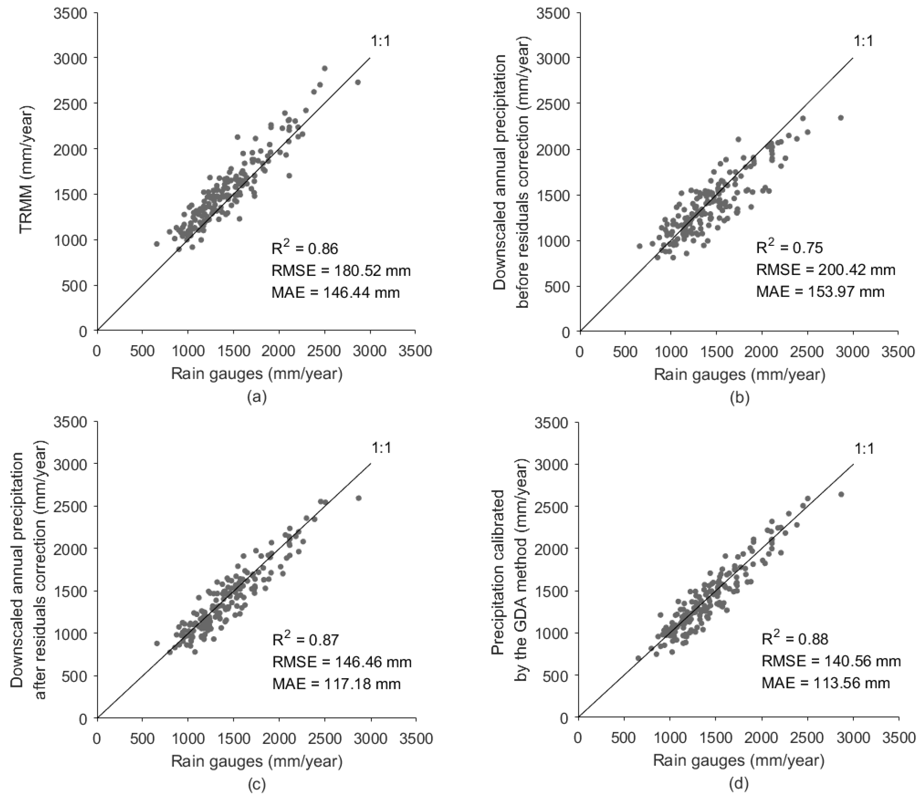
3.2. The Annual Downscaled Results and Ground Validation
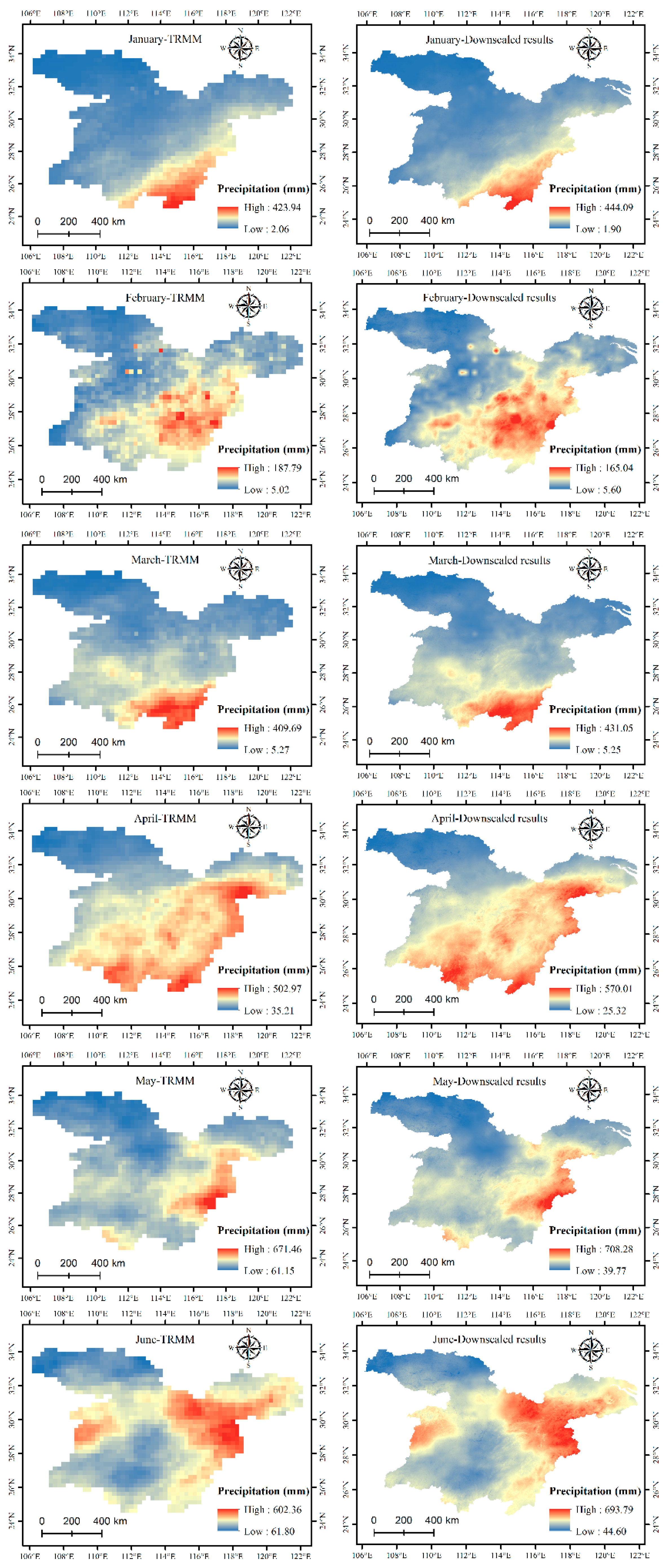
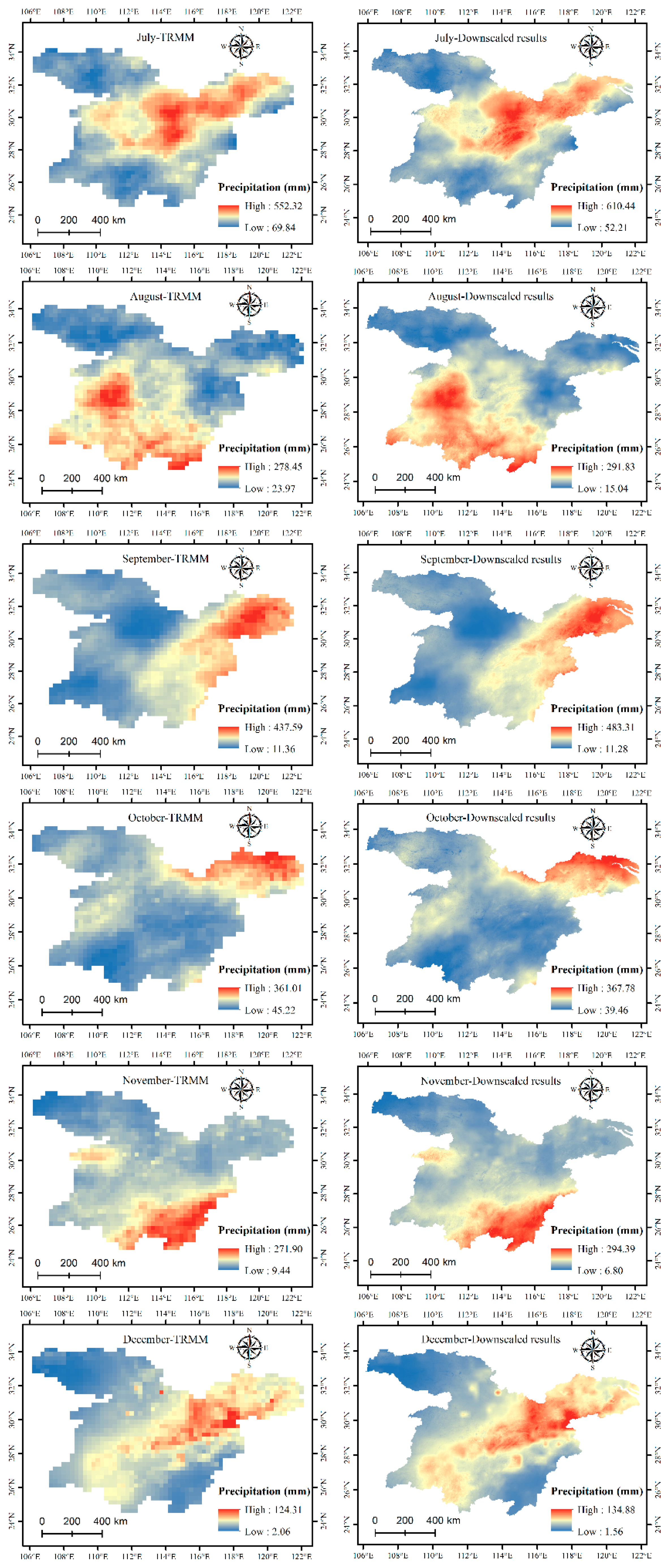
3.3. Downscaled Monthly Precipitation Results
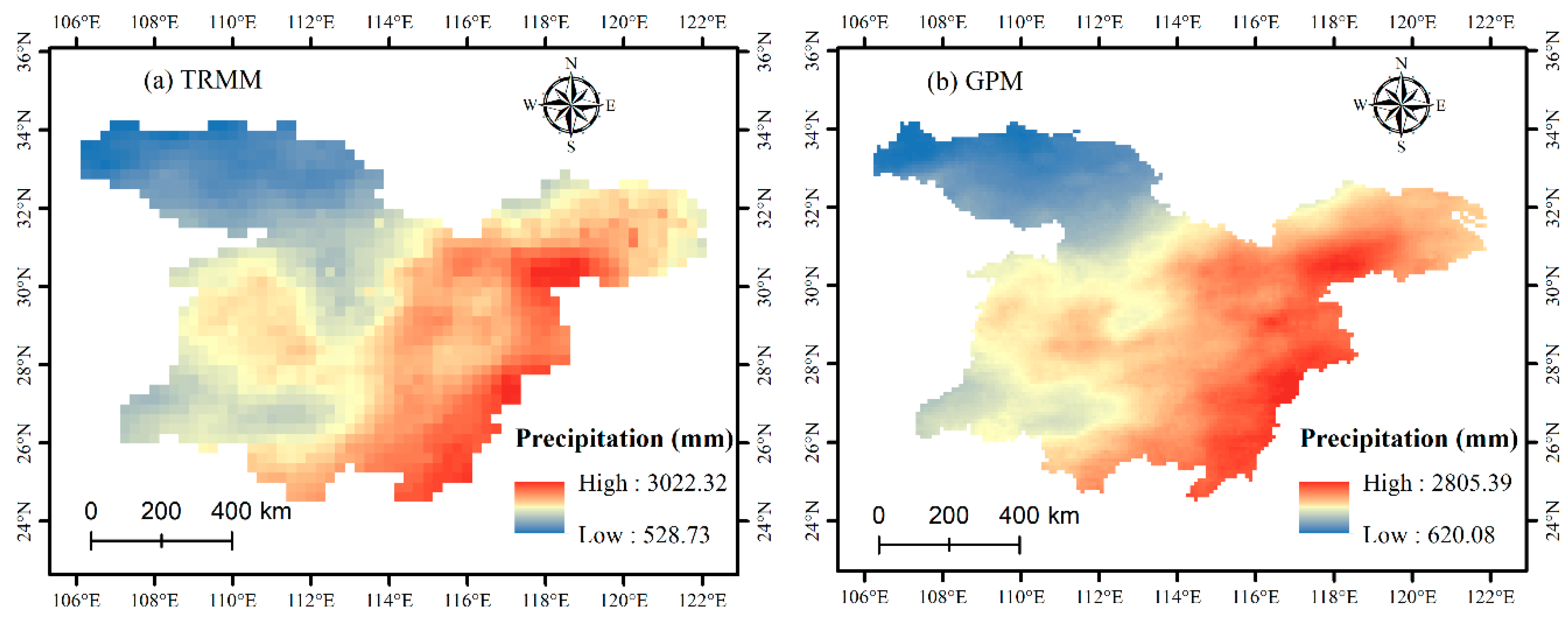
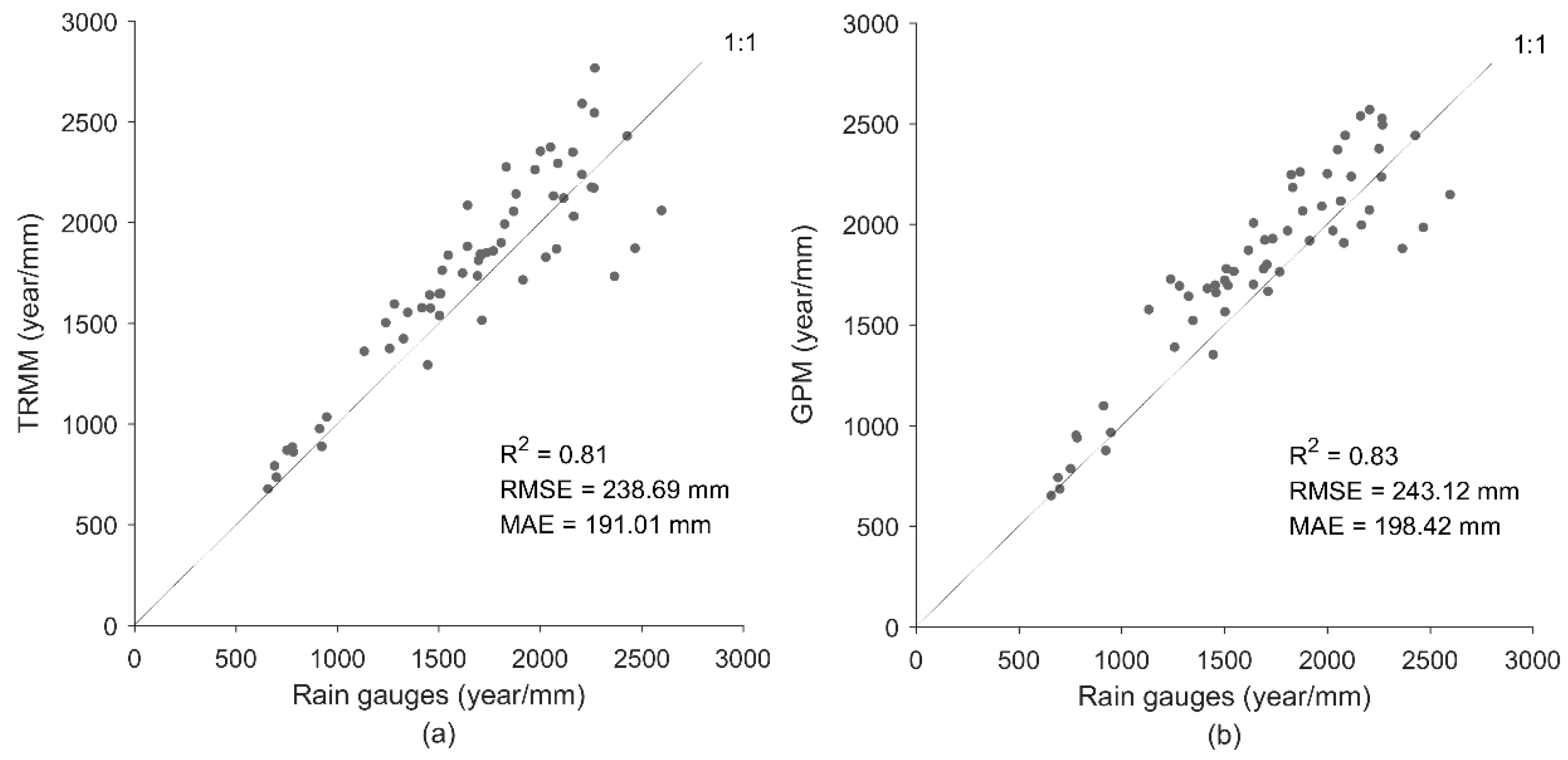
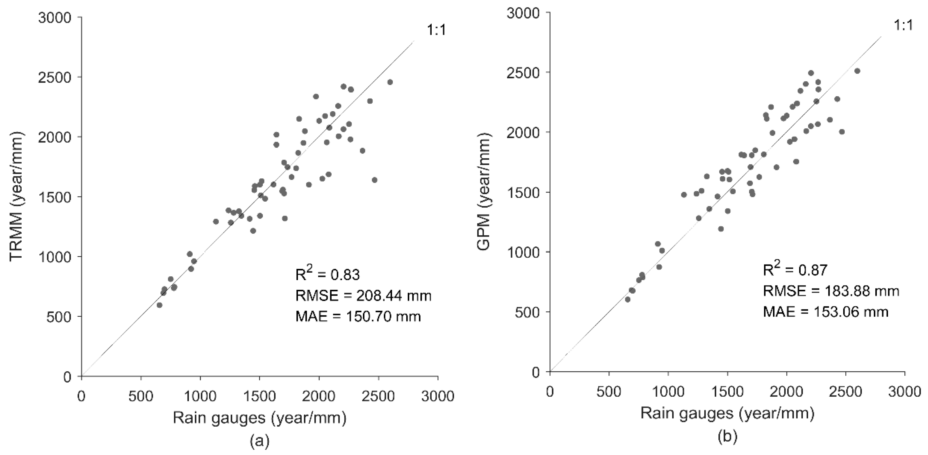
3.4. Comparison and Analysis of Downscaling Results of TRMM and GPM Data
4. Conclusions
- (1)
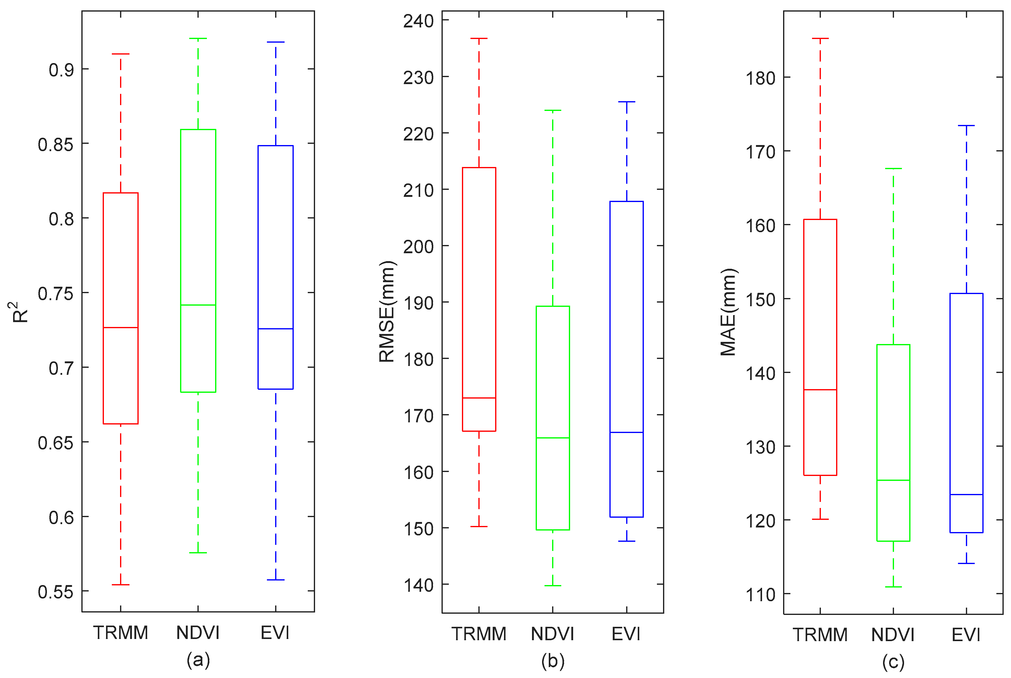
- We compared the accuracies of the annual downscaled results acquired with the NDVI-based and EVI-based GWR models, showing that the NDVI performed better than the EVI in the annual downscaling model. This may have been because this study used the annual average NDVI, which may have neutralized any detrimental saturation effects;
- (2)
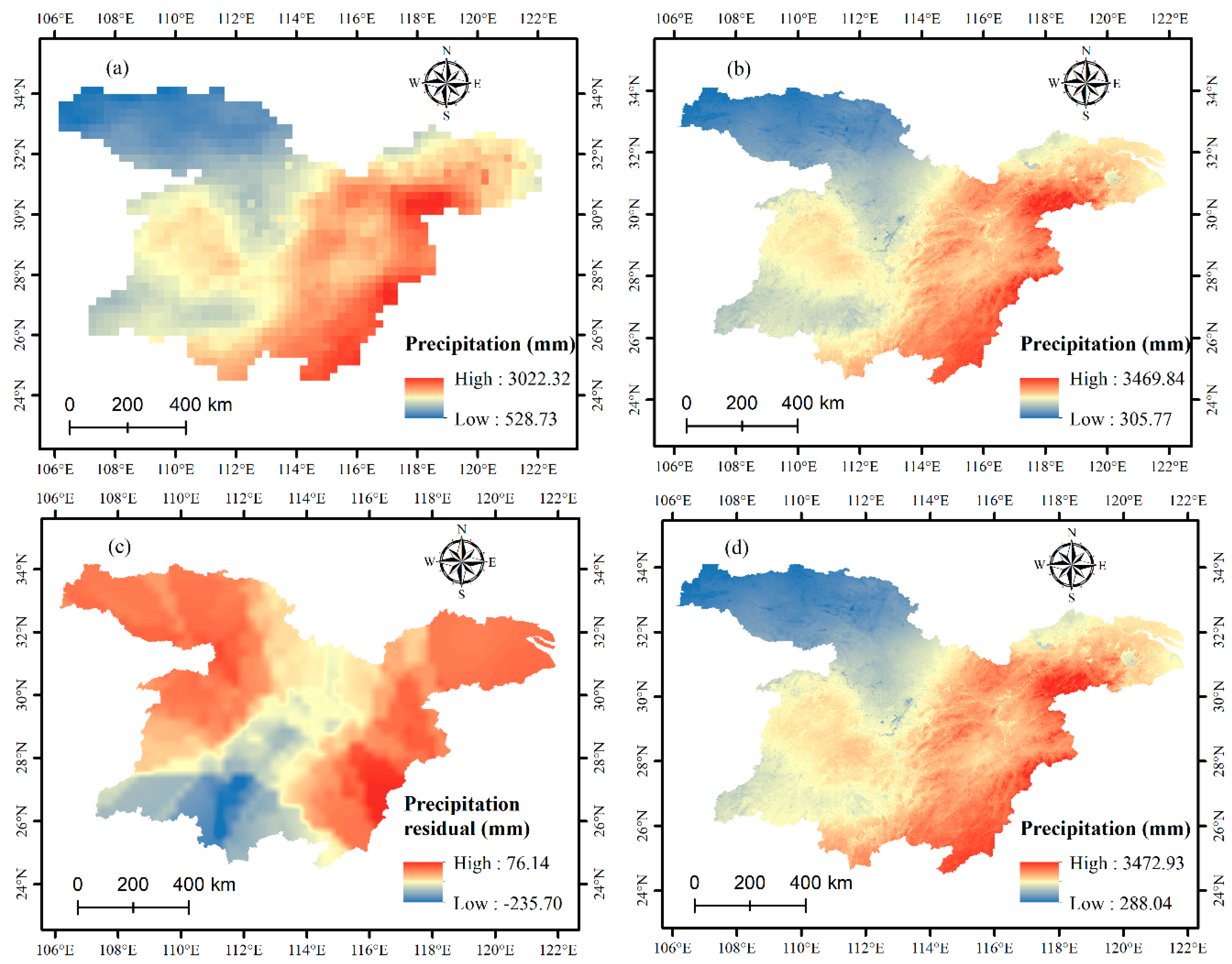
- The accuracy of the downscaling model could be effectively improved after correcting the residuals and performing a calibration with the GDA method. Subsequently, the calculated rainfall was closer to the actual weather station rainfall observations (R2 = 0.88, RMSE = 140.56 mm, and MAE = 113.56 mm). Thus, the calibration process was essential in providing more accurate downscaling results;
- (3)
- The downscaled results were decomposed into fractions to obtain monthly precipitation data. The downscaled method proposed in this study could improve not only the spatial resolution of remote sensing precipitation data, but also the accuracy of such data, by utilizing the GDA method;
- (4)
- Finally, we analyzed and compared the downscaling performance of TRMM data to GPM data over the MLRYRB. The results showed that the R2 and RMSE values of the GPM precipitation data (R2 = 0.87 and RMSE = 183.88 mm) were generally better than the TRMM precipitation data, but the MAE value of the former (MAE = 153.06 mm) was slightly larger than that of the latter.
Author Contributions
Funding
Acknowledgments
Conflicts of Interest
References
- Ma, Z.; Shi, Z.; Zhou, Y.; Xu, J.; Yu, W.; Yang, Y. A spatial data mining algorithm for downscaling TMPA 3B43 V7 data over the Qinghai–Tibet Plateau with the effects of systematic anomalies removed. Remote Sens. Environ. 2017, 200, 378–395. [Google Scholar] [CrossRef]
- Li, M.; Shao, Q. An improved statistical approach to merge satellite rainfall estimates and raingauge data. J. Hydrol. 2010, 385, 51–64. [Google Scholar] [CrossRef]
- Shi, Y.; Song, L.; Xia, Z.; Lin, Y.; Myneni, R.; Choi, S.; Wang, L.; Ni, X.; Lao, C.; Yang, F. Mapping annual precipitation across mainland China in the period 2001–2010 from TRMM3B43 product using spatial downscaling approach. Remote Sens. 2015, 7, 5849–5878. [Google Scholar] [CrossRef]
- Xu, G.; Xu, X.; Liu, M.; Sun, A.; Wang, K. Spatial downscaling of TRMM precipitation product using a combined multifractal and regression approach: Demonstration for South China. Water 2015, 7, 3083–3102. [Google Scholar] [CrossRef]
- Mahesh, C.; Prakash, S.; Sathiyamoorthy, V.; Gairola, R.M. Artificial neural network based microwave precipitation estimation using scattering index and polarization corrected temperature. Atmos. Res. 2011, 102, 358–364. [Google Scholar] [CrossRef]
- Zhu, H.; Li, Y.; Huang, Y.; Li, Y.; Hou, C.; Shi, X. Evaluation and hydrological application of satellite-based precipitation datasets in driving hydrological models over the Huifa river basin in Northeast China. Atmos. Res. 2018, 207, 28–41. [Google Scholar] [CrossRef]
- Behrangi, A.; Khakbaz, B.; Jaw, T.C.; AghaKouchak, A.; Hsu, K.; Sorooshian, S. Hydrologic evaluation of satellite precipitation products over a mid-size basin. J. Hydrol. 2011, 397, 225–237. [Google Scholar] [CrossRef]
- Kubota, T.; Shige, S.; Hashizume, H.; Aonashi, K.; Takahashi, N.; Seto, S.; Hirose, M.; Takayabu, Y.N.; Ushio, T.; Nakagawa, K.; et al. Global precipitation map using satellite-borne microwave radiometers by the GSMaP project: Production and validation. IEEE Trans. Geosci. Remote Sens. 2007, 45, 2259–2275. [Google Scholar] [CrossRef]
- Huffman, G.J.; Adler, R.F.; Arkin, P.; Chang, A.; Ferraro, R.; Gruber, A.; Janowiak, J.; McNab, A.; Rudolf, B.; Schneider, U. The global precipitation climatology project (GPCP) combined precipitation dataset. Bull. Am. Meteorol. Soc. 1997, 78, 5–20. [Google Scholar] [CrossRef]
- Adler, R.F.; Huffman, G.J.; Chang, A.; Ferraro, R.; Xie, P.P.; Janowiak, J.; Rudolf, B.; Schneider, U.; Curtis, S.; Bolvin, D.; et al. The version-2 global precipitation climatology project (GPCP) monthly precipitation analysis (1979–present). J. Hydrometeorol. 2003, 4, 1147–1167. [Google Scholar] [CrossRef]
- Huffman, G.J.; Bolvin, D.T.; Nelkin, E.J.; Wolff, D.B.; Adler, R.F.; Gu, G.; Hong, Y.; Bowman, K.P.; Stocker, E.F. The TRMM multisatellite precipitation analysis (TMPA): Quasi-global, multiyear, combined-sensor precipitation estimates at fine scales. J. Hydrometeorol. 2007, 8, 38–55. [Google Scholar] [CrossRef]
- Su, F.; Hong, Y.; Lettenmaier, D.P. Evaluation of TRMM multisatellite precipitation analysis (TMPA) and its utility in hydrologic prediction in the La Plata Basin. J. Hydrometeorol. 2008, 9, 622–640. [Google Scholar] [CrossRef]
- Sohn, B.J.; Han, H.-J.; Seo, E.-K. Validation of satellite-based high-resolution rainfall products over the Korean Peninsula using data from a dense rain gauge network. J. Appl. Meteorol. Climatol. 2010, 49, 701–714. [Google Scholar] [CrossRef]
- Zhan, C.; Han, J.; Hu, S.; Liu, L.; Dong, Y. Spatial downscaling of GPM annual and monthly precipitation using regression-based algorithms in a mountainous area. Adv. Meteorol. 2018, 2018, 1506017. [Google Scholar] [CrossRef]
- Zhang, Y.; Li, Y.; Ji, X.; Luo, X.; Li, X. Fine-resolution precipitation mapping in a mountainous watershed: Geostatistical downscaling of TRMM products based on environmental variables. Remote Sens. 2018, 10, 119. [Google Scholar] [CrossRef]
- Jia, S.; Zhu, W.; Lű, A.; Yan, T. A statistical spatial downscaling algorithm of TRMM precipitation based on NDVI and DEM in the Qaidam Basin of China. Remote Sens. Environ. 2011, 115, 3069–3079. [Google Scholar] [CrossRef] [Green Version]
- Immerzeel, W.W.; Rutten, M.M.; Droogers, P. Spatial downscaling of TRMM precipitation using vegetative response on the Iberian Peninsula. Remote Sens. Environ. 2009, 113, 362–370. [Google Scholar] [CrossRef]
- Ulloa, J.; Ballari, D.; Campozano, L.; Samaniego, E. Two-step downscaling of TRMM 3b43 V7 precipitation in contrasting climatic regions with sparse monitoring: The case of Ecuador in tropical South America. Remote Sens. 2017, 9, 758. [Google Scholar] [CrossRef]
- Ezzine, H.; Bouziane, A.; Ouazar, D.; Hasnaoui, M.D. Downscaling of TRMM3B43 product through spatial and statistical analysis based on normalized difference water index, elevation, and distance from sea. IEEE Geosci. Remote Sens. Lett. 2017, 14, 1449–1453. [Google Scholar] [CrossRef]
- Brunsdon, C.; McClatchey, J.; Unwin, D.J. Spatial variations in the average rainfall-altitude relationship in Great Britain: An approach using geographically weighted regression. Int. J. Climatol. 2001, 21, 455–466. [Google Scholar] [CrossRef]
- Pettorelli, N.; Vik, J.O.; Mysterud, A.; Gaillard, J.M.; Tucker, C.J.; Stenseth, N.C. Using the satellite-derived NDVI to assess ecological responses to environmental change. Trends Ecol. Evol. 2005, 20, 503–510. [Google Scholar] [CrossRef] [PubMed]
- Fang, J.; Du, J.; Xu, W.; Shi, P.; Li, M.; Ming, X. Spatial downscaling of TRMM precipitation data based on the orographical effect and meteorological conditions in a mountainous area. Adv. Water Resour. 2013, 61, 42–50. [Google Scholar] [CrossRef]
- Foody, G.M. Geographical weighting as a further refinement to regression modelling: An example focused on the NDVI–rainfall relationship. Remote Sens. Environ. 2003, 88, 283–293. [Google Scholar] [CrossRef]
- Gao, J.; Li, S. Detecting spatially non-stationary and scale-dependent relationships between urban landscape fragmentation and related factors using Geographically Weighted Regression. Appl. Geogr. 2011, 31, 292–302. [Google Scholar] [CrossRef]
- Brunsdon, C.; Fotheringham, A.S.; Charlton, M.E. Geographically weighted regression: A method for exploring spatial nonstationarity. Geogr. Anal. 1996, 28, 281–298. [Google Scholar] [CrossRef]
- An, K.-J.; Lee, S.-W.; Hwang, S.-J.; Park, S.-R.; Hwang, S.-A. Exploring the non-stationary effects of forests and developed land within watersheds on biological indicators of streams using geographically-weighted regression. Water 2016, 8, 120. [Google Scholar] [CrossRef]
- Li, S.; Zhao, Z.; Miaomiao, X.; Wang, Y. Investigating spatial non-stationary and scale-dependent relationships between urban surface temperature and environmental factors using geographically weighted regression. Environ. Model. Softw. 2010, 25, 1789–1800. [Google Scholar] [CrossRef]
- Huete, A.; Didan, K.; Miura, T.; Rodriguez, E.P.; Gao, X.; Ferreira, L.G. Overview of the radiometric and biophysical performance of the MODIS vegetation indices. Remote Sens. Environ. 2002, 83, 195–213. [Google Scholar] [CrossRef]
- Justice, C.O.; Vermote, E.; Townshend, J.R.G.; Defries, R.; Roy, D.P.; Hall, D.K.; Salomonson, V.V.; Privette, J.L.; Riggs, G.; Strahler, A.; et al. The Moderate Resolution Imaging Spectroradiometer (MODIS): Land remote sensing for global change research. IEEE Trans. Geosci. Remote Sens. 1998, 36, 1228–1249. [Google Scholar] [CrossRef]
- Zhang, T.; Gong, W.; Wang, W.; Ji, Y.; Zhu, Z.; Huang, Y. Ground level PM2.5 estimates over China using satellite-based geographically weighted regression (GWR) models are improved by including NO2 and enhanced vegetation index (EVI). Int. J. Environ. Res. Public Health 2016, 13, 1215. [Google Scholar] [CrossRef] [PubMed]
- Shi, Y.L.; Song, L. Spatial downscaling of monthly TRMM precipitation based on EVI and other geospatial variables over the Tibetan Plateau From 2001 to 2012. Mt. Res. Dev. 2015, 35, 180–194. [Google Scholar] [CrossRef]
- Chen, S.; Zhang, L.; Liu, X.; Guo, M.; She, D. The Use of SPEI and TVDI to assess temporal-spatial variations in drought conditions in the middle and lower reaches of the Yangtze River Basin, China. Adv. Meteorol. 2018, 2018, 9362041. [Google Scholar] [CrossRef]
- De Jesús, A.; Breña-Naranjo, J.; Pedrozo-Acuña, A.; Alcocer Yamanaka, V. The use of TRMM 3B42 product for drought monitoring in Mexico. Water 2016, 8, 325. [Google Scholar] [CrossRef]
- Moazami, S.; Golian, S.; Kavianpour, M.R.; Hong, Y. Uncertainty analysis of bias from satellite rainfall estimates using copula method. Atmos. Res. 2014, 137, 145–166. [Google Scholar] [CrossRef]
- Wallace, C.; Walker, J.; Skirvin, S.; Patrick-Birdwell, C.; Weltzin, J.; Raichle, H. Mapping presence and predicting phenological status of invasive buffelgrass in Southern Arizona using MODIS, climate and citizen science observation data. Remote Sens. 2016, 8, 524. [Google Scholar] [CrossRef]
- Scharlemann, J.P.; Benz, D.; Hay, S.I.; Purse, B.V.; Tatem, A.J.; Wint, G.R.; Rogers, D.J. Global data for ecology and epidemiology: A novel algorithm for temporal Fourier processing MODIS data. PLoS ONE 2008, 3, e1408. [Google Scholar] [CrossRef]
- Eckert, S.; Hüsler, F.; Liniger, H.; Hodel, E. Trend analysis of MODIS NDVI time series for detecting land degradation and regeneration in Mongolia. J. Arid Environ. 2015, 113, 16–28. [Google Scholar] [CrossRef]
- Ning, S.; Wang, J.; Jin, J.; Ishidaira, H. Assessment of the latest GPM-Era high-resolution satellite precipitation products by comparison with observation gauge data over the Chinese mainland. Water 2016, 8, 481. [Google Scholar] [CrossRef]
- Shahabfar, A.; Eitzinger, J. Agricultural drought monitoring in semi-arid and arid areas using MODIS data. J. Agric. Sci. 2011, 149, 403–414. [Google Scholar] [CrossRef]
- Xu, S.; Wu, C.; Wang, L.; Gonsamo, A.; Shen, Y.; Niu, Z. A new satellite-based monthly precipitation downscaling algorithm with non-stationary relationship between precipitation and land surface characteristics. Remote Sens. Environ. 2015, 162, 119–140. [Google Scholar] [CrossRef]
- Brunsdon, C.; Fotheringham, A.S.; Charlton, M. Some notes on parametric significance tests for geographically weighted regression. J. Reg. Sci. 1999, 39, 497–524. [Google Scholar] [CrossRef]
- Tu, J.; Xia, Z.G. Examining spatially varying relationships between land use and water quality using geographically weighted regression I: Model design and evaluation. Sci. Total Environ. 2008, 407, 358–378. [Google Scholar] [CrossRef] [PubMed]
- Chen, Y.; Huang, J.; Sheng, S.; Mansaray, L.R.; Liu, Z.; Wu, H.; Wang, X. A new downscaling-integration framework for high-resolution monthly precipitation estimates: Combining rain gauge observations, satellite-derived precipitation data and geographical ancillary data. Remote Sens. Environ. 2018, 214, 154–172. [Google Scholar] [CrossRef]
- Cheema, M.J.M.; Bastiaanssen, W.G.M. Local calibration of remotely sensed rainfall from the TRMM satellite for different periods and spatial scales in the Indus Basin. Int. J. Remote Sens. 2012, 33, 2603–2627. [Google Scholar] [CrossRef]
- Laurent, L.; Audois, P.; Marie-Joseph, I.; Becker, M.; Seyler, F. Calibration of TRMM 3B42 with geographical differential analysis over North Amazonia. In Proceedings of the 2013 IEEE International Geoscience and Remote Sensing Symposium—IGARSS, Melbourne, VIC, Australia, 21–26 July 2013; pp. 2234–2237. [Google Scholar] [CrossRef]
- Duan, Z.; Bastiaanssen, W.G.M. First results from Version 7 TRMM 3B43 precipitation product in combination with a new downscaling–calibration procedure. Remote Sens. Environ. 2013, 131, 1–13. [Google Scholar] [CrossRef]
- Omranian, E.; Sharif, H.O. Evaluation of the global precipitation measurement (GPM) satellite rainfall products over the lower Colorado River Basin, Texas. JAWRA J. Am. Water Resour. Assoc. 2018, 54, 882–898. [Google Scholar] [CrossRef]


| Weather Station Name | Longitude | Latitude | Elevation | TRMM | Downscaled Results | ||||
|---|---|---|---|---|---|---|---|---|---|
| R2 | RMSE | MAE | R2 | RMSE | MAE | ||||
| Yichang | 111.30 | 30.70 | 105 | 0.90 | 29.73 | 20.18 | 0.90 | 25.80 | 16.99 |
| Wuhan | 114.13 | 30.62 | 14 | 0.91 | 28.85 | 18.72 | 0.93 | 26.23 | 17.89 |
| Yueyang | 113.08 | 29.38 | 19 | 0.78 | 42.26 | 31.44 | 0.84 | 32.48 | 22.83 |
| Anhua | 111.22 | 28.38 | 201 | 0.83 | 43.95 | 26.66 | 0.85 | 43.55 | 27.99 |
| Jian | 114.92 | 27.05 | 44 | 0.84 | 41.61 | 29.85 | 0.84 | 40.83 | 29.34 |
| Wugang | 110.63 | 26.73 | 338 | 0.91 | 23.52 | 17.10 | 0.91 | 21.89 | 16.08 |
| Chenzhou | 113.03 | 25.80 | 179 | 0.86 | 37.51 | 25.38 | 0.87 | 35.52 | 23.45 |
| Chaohu | 117.87 | 31.62 | 21 | 0.74 | 44.40 | 28.14 | 0.76 | 41.68 | 23.05 |
| Boyang | 116.68 | 29.00 | 20 | 0.79 | 50.54 | 32.72 | 0.82 | 44.71 | 29.78 |
| Nancheng | 116.65 | 27.58 | 64 | 0.92 | 37.67 | 26.69 | 0.92 | 33.65 | 23.82 |
© 2019 by the authors. Licensee MDPI, Basel, Switzerland. This article is an open access article distributed under the terms and conditions of the Creative Commons Attribution (CC BY) license (http://creativecommons.org/licenses/by/4.0/).
Share and Cite
Chen, S.; Zhang, L.; She, D.; Chen, J. Spatial Downscaling of Tropical Rainfall Measuring Mission (TRMM) Annual and Monthly Precipitation Data over the Middle and Lower Reaches of the Yangtze River Basin, China. Water 2019, 11, 568. https://doi.org/10.3390/w11030568
Chen S, Zhang L, She D, Chen J. Spatial Downscaling of Tropical Rainfall Measuring Mission (TRMM) Annual and Monthly Precipitation Data over the Middle and Lower Reaches of the Yangtze River Basin, China. Water. 2019; 11(3):568. https://doi.org/10.3390/w11030568
Chicago/Turabian StyleChen, Shaodan, Liping Zhang, Dunxian She, and Jie Chen. 2019. "Spatial Downscaling of Tropical Rainfall Measuring Mission (TRMM) Annual and Monthly Precipitation Data over the Middle and Lower Reaches of the Yangtze River Basin, China" Water 11, no. 3: 568. https://doi.org/10.3390/w11030568