The Impacts of Spatially Variable Demand Patterns on Water Distribution System Design and Operation

Abstract

Resilient water distribution systems (WDSs) need to minimize the level of service failure in terms of magnitude and duration over its design life when subject to exceptional conditions. This requires WDS design to consider scenarios as close as possible to real conditions of the WDS to avoid any unexpected level of service failure in future operation (e.g., insufficient pressure, much higher operational cost, water quality issues, etc.). Thus, this research aims at exploring the impacts of design flow scenarios (i.e., spatial-variant demand patterns) on water distribution system design and operation. WDSs are traditionally designed by using a uniform demand pattern for the whole system. Nevertheless, in reality, the patterns are highly related to the number of consumers, service areas, and the duration of peak flows. Thus, water distribution systems are comprised of distribution blocks (communities) organized in a hierarchical structure. As each community may be significantly different from the others in scale and water use, the WDSs have spatially variable demand patterns. Hence, there might be considerable variability of real flow patterns for different parts of the system. Consequently, the system operation might not reach the expected performance determined during the design stage, since all corresponding facilities are commonly tailor-made to serve the design flow scenario instead of the real situation. To quantify the impacts, WDSs’ performances under both uniform and spatial distributed patterns are compared based on case studies. The corresponding impacts on system performances are then quantified based on three major metrics; i.e., capital cost, energy cost, and water quality. This study exemplifies that designing a WDS using spatial distributed demand patterns might result in decreased life-cycle cost (i.e., lower capital cost and nearly the same pump operating cost) and longer water ages. The outcomes of this study provide valuable information regarding design and operation of water supply infrastructures; e.g., assisting the optimal design.

1. Introduction

Build resilience in infrastructure systems is an emerging need for the aim of sustainable development. However, how to design a resilient infrastructure system is still an open question. Here, the resilience is defined as the degree to which the system minimizes level of service failure magnitude and duration, and maximizes the time to level of service failure, over its design life when subject to exceptional conditions (reproduced based on [1]). Apparently, the worst case would be that the designed system directly fails to serve as expected after implementation in practice. This may happen if the design scenarios considered have non-marginal differences from the real conditions, and thus make the real conditions unexpected. To quantify the impacts resulting from the differences and thus provide references for resilient design, this paper will focus on water distribution systems (WDSs), the lifeline of a city that delivers potable water from sources to water users.

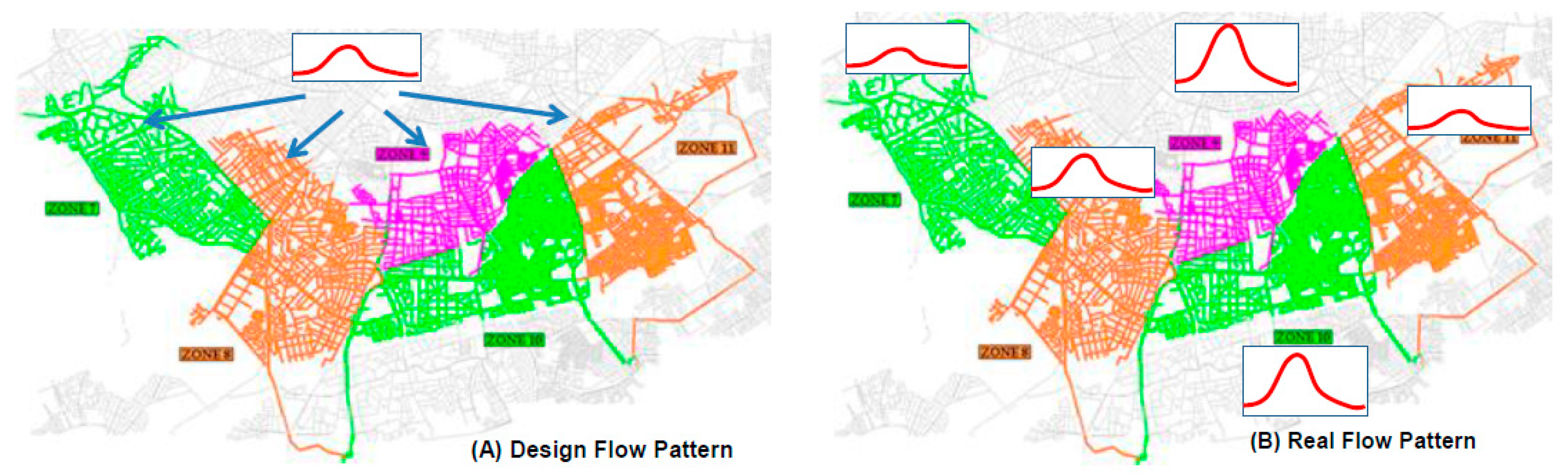
Design of WDSs requires estimation of the demand pattern. A demand pattern describes the variation of the amount of water used by the system over time (e.g., hour, day, and season [2]) and is hence related to the system’s capacity, energy consumption, and water quality. Traditionally, WDSs are designed by using a uniform demand pattern for the whole system. Nevertheless, except for the time variations, in reality the patterns may also have considerable spatial variations; i.e., there may be considerable differences among real flow patterns in different parts of the system even if the total consumption is similar [2,3] (Figure 1). For example, the flow pattern of a small rural region may fluctuate frequently while it has a low peak flow. Contrarily, the flow pattern of an urban area may be steady but has a rather high peak flow. Consequently, despite the total demand of the WDS being well-estimated, ignoring the spatial distribution of the demand may still cause negative system-wide influences on performances of WDSs (e.g., insufficient pressure, much higher operational cost, water quality issues, etc.), if there are non-negligible differences between demand patterns used at the design stage and the real patterns. Thus, design resilient WDSs require research to further explore the impacts of spatial variability of demands on the WDS design.

The spatial variability of water demands derives from the mechanism of water distribution system development. Typically, groups of customers are organized as communities due to urban planning. WDSs are expanding with the evolution of urban environments and are therefore developed in a community by community manner [4,5,6]. As each community may be significantly different from the others in scale and water use, the WDSs are systems with community-specific demand patterns. However, frequently a deeper understanding of the spatial demand distribution is limited due to insufficient availability and information content of water records. Recently, Kanakoudis et al. developed an innovative method for spatial demand allocation in WDS and proved it is more accurate than the multiplicatively-weighted-Voronoi diagram method (using population density based weighting factors) to enable more cost effective design of WDSs [7]. A study was carried out by Gora (2011) to determine the effects of variable water demands on water quality and use in a selection of communities that supply a large industrial user in addition to the usual assortment of residential, commercial, and institutional users [2]. Gora indicated in the report [2] that it is advocated to install flow meters/totalizers and do careful record-keeping among system operators to reduce designers’ reliance on assumed per capita values. Although water demand can be approximated using assumed per capita flow rates and peaking factors, this is not recommended as water use can vary significantly from one community to the next. Filion et al. [8] examined various design solutions of a benchmark WDS resulting from using a set of synthetic demand patterns statistically similar to the historical records, and revealed that standard deviation of pressure heads and capital costs can be sensitive to the level of cross correlation between nodal demands. Further, Filion [7] explored the relationship between the urban form of WDSs and their energy use. The Urban form corresponds to the network pipe configuration and the spatial distribution of water users. Diao et al. [9] tested corresponding system-wide influences on water age and energy consumption if the average and peak demands defined at the design stage are inconsistent with ones in real situations. Based on numerous case studies, Sitzenfrei et al. [10] examined how the demand patterns impact water age distributions by comparing results from simulations using demand patterns and hydraulic steady state simulations.

Accordingly, this research explores the impacts of spatially variable demand patterns on water distribution system design and operation. In this regard, case studies are carried out to test WDSs’ performance under both uniform and spatial distributed patterns. Here, application of the uniform distributed patterns represents the case of estimating water demand pattern at the low level of spatial resolution. The corresponding impacts of spatial refined patterns are then quantified based on three metrics; i.e. capital cost, energy cost, and water quality. The outcome of this study provides useful information regarding design and operation of water supply infrastructures. In the absence of actual data, the possible impacts could still be estimated using the procedure introduced in this study. Say, a set of demand patterns could be created for each of the communities, by estimation based on the communities’ service areas, populations, and water uses etc. Then, various combinations of those patterns could be used as inputs for model-based analyses. If designing a WDS using spatial distributed demand patterns has potential to reduce the life-cycle cost, a cost efficiency analysis can be made, comparing the possible saving with the extra costs for detailed metering and demand assessment.

2. Materials and Methods

Water distribution systems are expanding along with urban evolution and are therefore developed community by community. The evolution of urban environments starts from initial building blocks. These entities subsequently expand or combine with one another to form larger blocks (e.g., communities) step by step. During this process, water distribution pipes are organized following the development of the communities, and therefore the distribution systems are also formed community-wise. Thus, water distribution systems are comprised of distribution blocks (communities) organized in a hierarchical structure. As each community may be significantly different from the others in scale and water use, the WDSs have spatially variable demand patterns. Hence, there might be considerable variability of real flow patterns for different parts of the system. Consequently, the system operation might not reach the expected performance determined during the design stage, since all corresponding facilities are commonly tailor-made to serve the design flow scenario instead of the real situation. As for the impact of the spatial distributed demand patterns, in this study three hypotheses are made:

2.1. Hypothesis

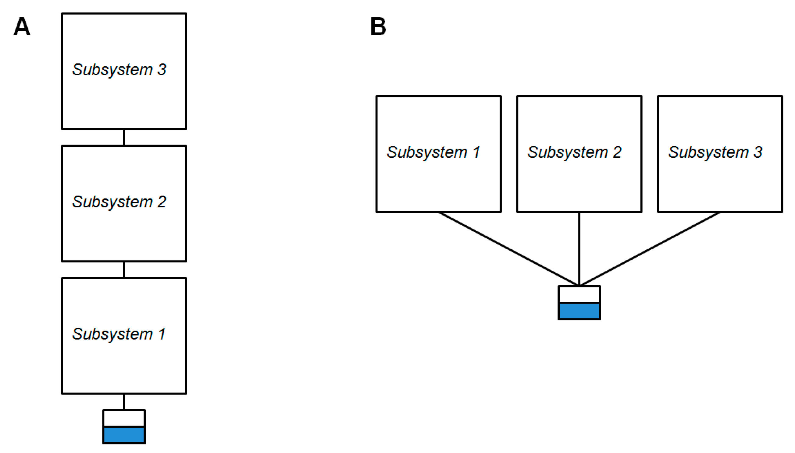
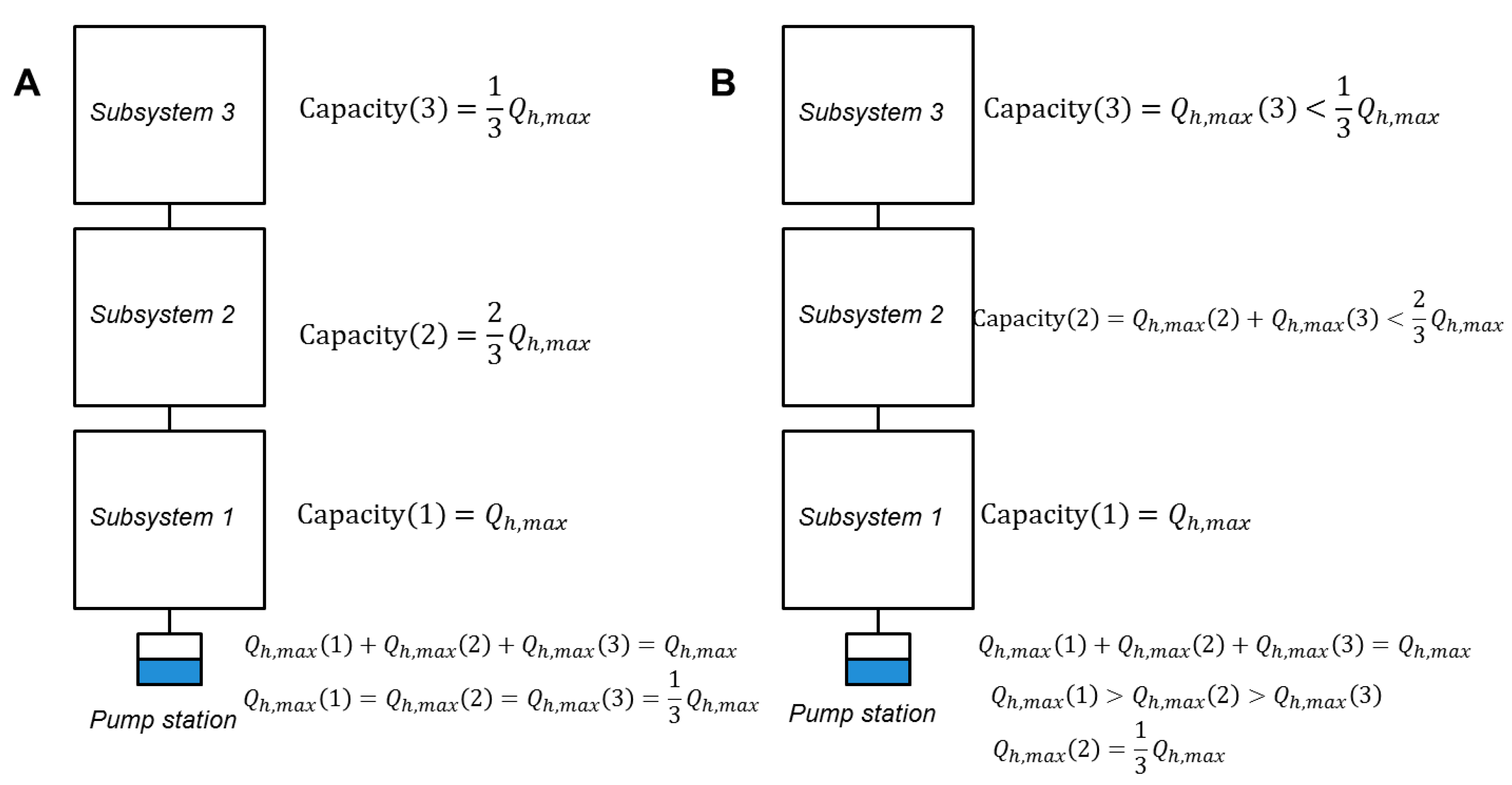
• By allowing capacity allocation at the community level, a design procedure using spatial distributed patterns eliminates potential pressure problems at communities with large water demands, and may reduce capital cost in the case of ideal demand distribution. The ideal distribution refers to the situation, in which a distribution system has all the communities following the altitudinal distribution (Figure 2A) and communities with highest peak demands are the nearest ones from the water source and vice versa. For instance, consider a distribution system with all three communities following the altitudinal distribution (Figure 3). The peak demand of the whole system is Q_h,max, and that of each community is Q_h,max(1), Q_h,max(2), and Q_h,max(3), respectively. Hence, the capacities of community 1–3 will be (Q_h,max(1) + Q_h,max(2) + Q_h,max(3) = Q_h,max) for community 1, (Q_h,max(2) + Q_h,max(3)) for community 2, and Q_h,max(3) for community 3. Apparently, smaller Q_h,max(2) and Q_h,max(3) will require smaller capacities in community 2 and 3, and thus decrease the capital cost of the WDSs(Figure 3B). If the community with the highest peak demand is the one furthest away from the pump station, however, capital cost saving is not guaranteed. The situation in longitudinal distribution (e.g., Figure 2B) would be more complicated. Hence, case studies are necessary to identify the complex interactions. However, in the case shown in Figure 2B it is predictable that if the WDN is designed by assuming equal demands at each subsystem, the subsystem with higher demand will have pressure deficiency.
• The water quality may deteriorate in spatial distributed systems, especially in communities that have more periods of low flow when the water retention time in the system increases.
• As for the energy cost, there might be no significant difference between a uniform distributed system and a spatial distributed system. This is because the average demands served are the same in both cases.

2.2. The Proposed Approach

To test the hypothesis, the proposed approach is to first create both uniform and distributed demand patterns. Next, optimal design of WDSs is carried out based on the two types of patterns, respectively. Finally, the design solutions are compared based on three metrics; i.e., capital cost, operational cost, and water quality. Detailed methodology is introduced below.

2.2.1. Creation of Spatial Demand Patterns

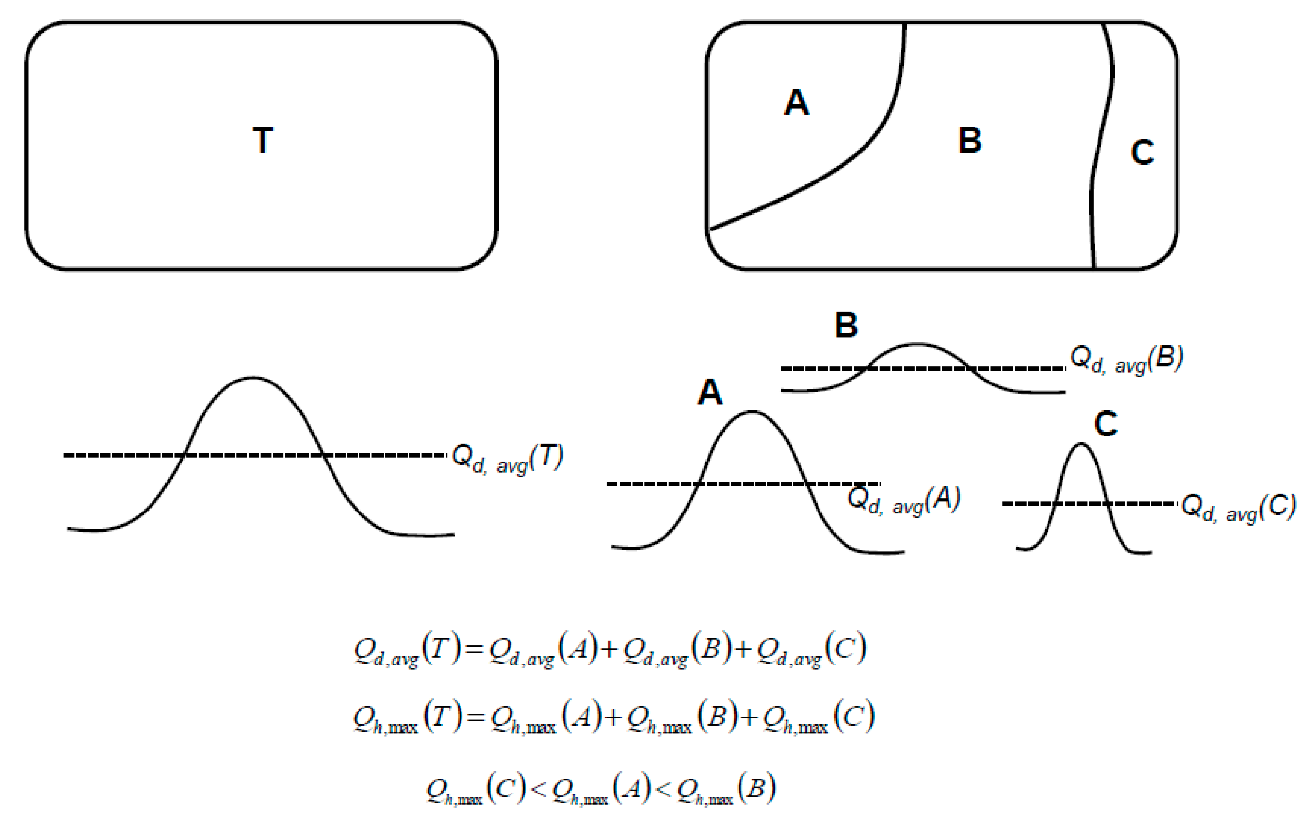
In this study, the spatial distribution of demands is represented by decomposing the uniform pattern of a WDS into several subsets. Each one of them refers to one community. The average demand (Q_d,avg) and peak demand (Q_h,max) remains unchanged on a system-wide level, while it differs on a community level. As Figure 4 shows, the decomposition is made on an example system, consisting of three communities (could also refer to subsystems), for further illustration.

2.2.2. Optimal Design

The optimal design in this study is formulated as a single objective optimization problem, which aims at minimizing the capital cost and meanwhile satisfies performance requirements via proper pipe sizing. The decision variables are diameters for all the pipes in the WDSs, and the performance constraints include minimum allowed pressure and an acceptable range of velocities. The general model formulation is shown as Equations (1)–(5):

$$\mathrm{Minimize}Cost={{\displaystyle \sum }}_{i\in NP}{c}_i\left(d_i,L_i\right)$$

(1)

Subject to

$${\displaystyle \sum _{i\in N{P}_{\mathrm{in},n}}{Q}_i}-{\displaystyle \sum _{j\in N{P}_{\mathrm{out},n}}{Q}_j=D_n},\forall n\in NN$$

(2)

$${\displaystyle \sum _{k\in \mathrm{Loop}p}{h}_k}=0,\forall p\in NL$$

(3)

$$H_n\ge H_{n\min },\forall n\in NN$$

(4)

$$V_{k\min }\le V_k\le V_{k\max },\forall k\in NP$$

(5)

where c_i (d_i, L_i)―cost of the pipe i with diameter d_i and length L_i; Q―pipe flow; h―pipe head loss; H―nodal head; NN―node set; NP―pipe set; NP_in,n―set of pipes entering node n; NP_out,n―set of pipes leaving node n; NL―loop set; ND―discrete commercial diameter set; D―nodal demand; H_min―minimum acceptable nodal head; V_min―minimum acceptable velocity; V_max―maximum acceptable velocity; c―unit cost per length.

3. Case Studies

Two case studies are analyzed using the proposed methodology to verify the three hypotheses mentioned above.

3.1. Case Study One

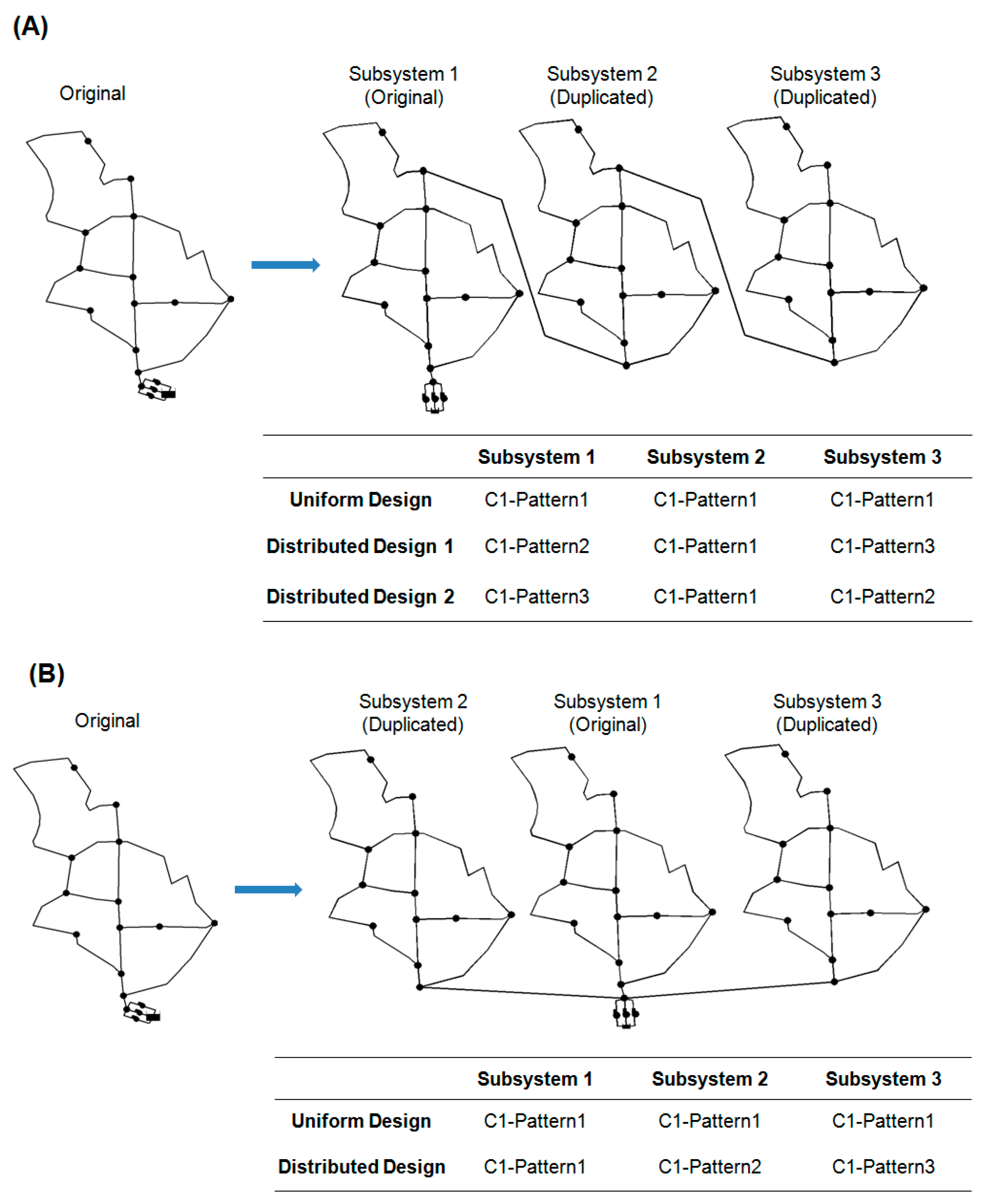
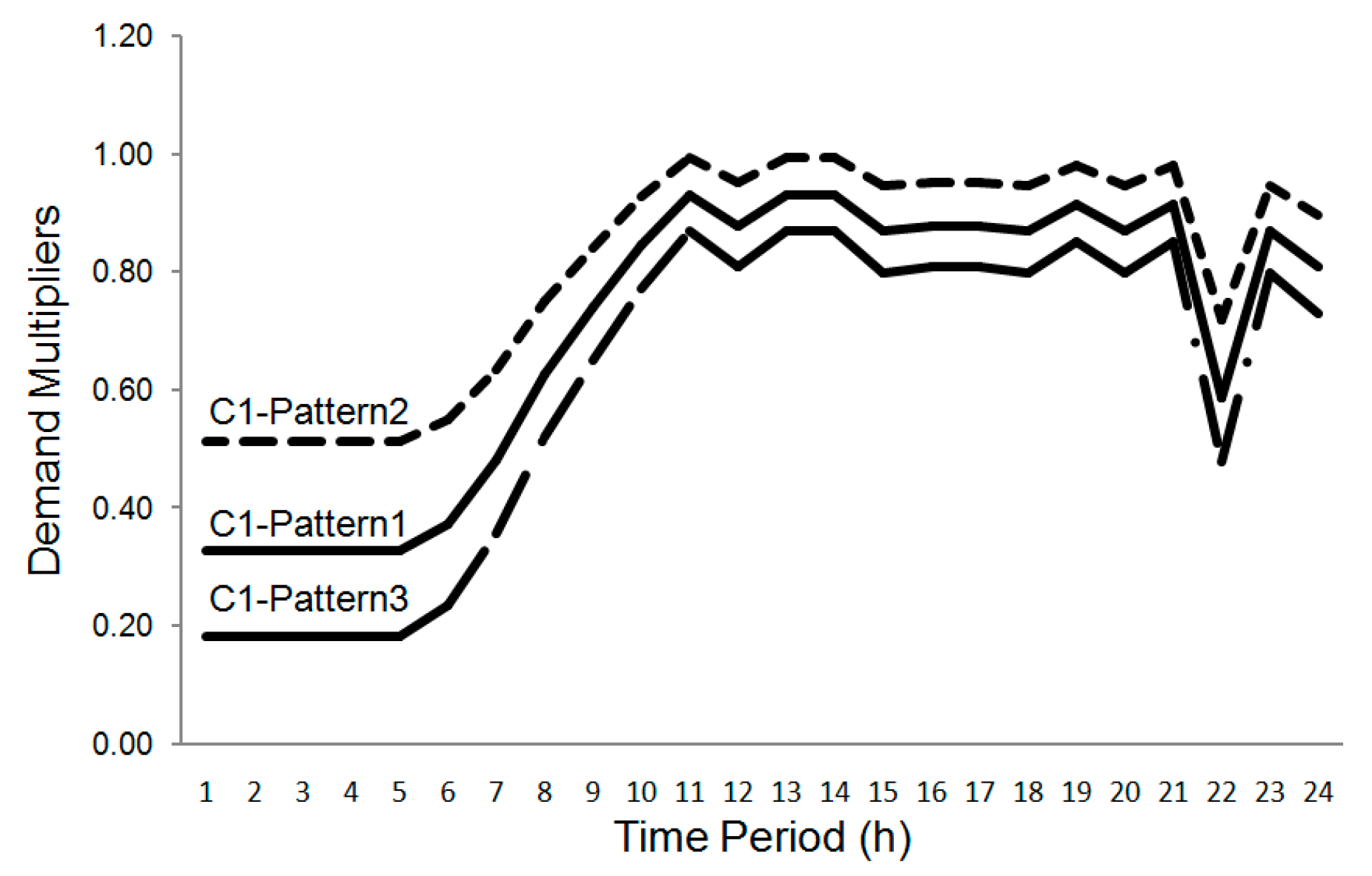
As Figure 5 shows, the case study focuses on two virtual systems, which are created by duplicating a smaller water distribution network [9]. The two case study networks are composed of three communities, spatially organized into either longitudinal form (Figure 5A) or altitudinal form (Figure 5B), respectively. With regard to the service region, the total population is around 60,000, and the supply area is about 600 hectares. A simple energy tariff (0.1 €/KWh) is used. For the “Uniform” design of the two systems, C1-Pattern1 is applied (Figure 6). The pattern represents the variation of water use on the maximum consumption day. For the “Distributed” design, two new demand patterns (C1-Pattern 2 and 3) are generated by scaling the C1-Pattern1. As a next step, each community is assigned a unique demand pattern (Figure 6). Note that the three patterns satisfy the constraints specified in the process of demand pattern decomposition.

The network is designed by utilizing WaterNetGen [11], an EPANET [12] extension for automatic Water Distribution Network models generation. The tool implements the Simulated Annealing algorithm [11,13,14] for optimal design. For all case studies, the commercial diameter set provided in

Table 1. Unit pipe prices (c). Ductile cast iron pipe, with Tyton (a trademark) Joint, Purchase Quantity over 10 tonnes, Delivery and Laying.

Diameter (mm)	80	100	150	200	250	300	400	500	600
Unit cost (€/m)	33	38	55	75	95	115	175	230	300

is used for pipe sizing. Besides, to implement the simulated annealing method, default values are used for the four essential parameters; i.e., a = 0.1, n₁ = (40, 30, 20, 10), r = (0.90, 0.80, 0.70, 0.50), n₂ = 2. For more information regarding to the parameters, please refer to the detailed instructions provided by Cunha and Sousa [14,15]. To facilitate illustration, the auto-designed networks are named as “Uniform” (using uniform distributed patterns) and “Distributed” (using spatial distributed patterns) respectively. Correspondingly, the two design strategies refer to “Uniform” design and “Distributed” design. In both cases, the same constraints on pressure and velocity are imposed; i.e., H ≥ 26 m (255 kPa) and 0.1 m/s ≤ V ≤ 10 m/s. For the altitudinal distribution, both the ideal and worst distribution is investigated. Here, the ideal distribution refers to distributed design 1 in Figure 5B, as subsystem 3 (with the highest peak demand) is the nearest one from the pump station and vice versa for subsystem 1 (with the lowest peak demand). Contrarily, distributed design 2 considers the worst distribution. For the longitudinal distribution, the uniformed and distributed design in Figure 5B is implemented.

Capital cost, water quality, and energy consumption are the three metrics for evaluation. In terms of capital cost, it is calculated based on Table 1. In terms of water quality, water age is chosen as a suitable surrogate indicator [16]. In terms of energy consumption, pump operating cost is calculated based on corresponding electrical tariffs. A 96 h simulation period is used to ensure stable periodical water age.

3.2. Case Study Two

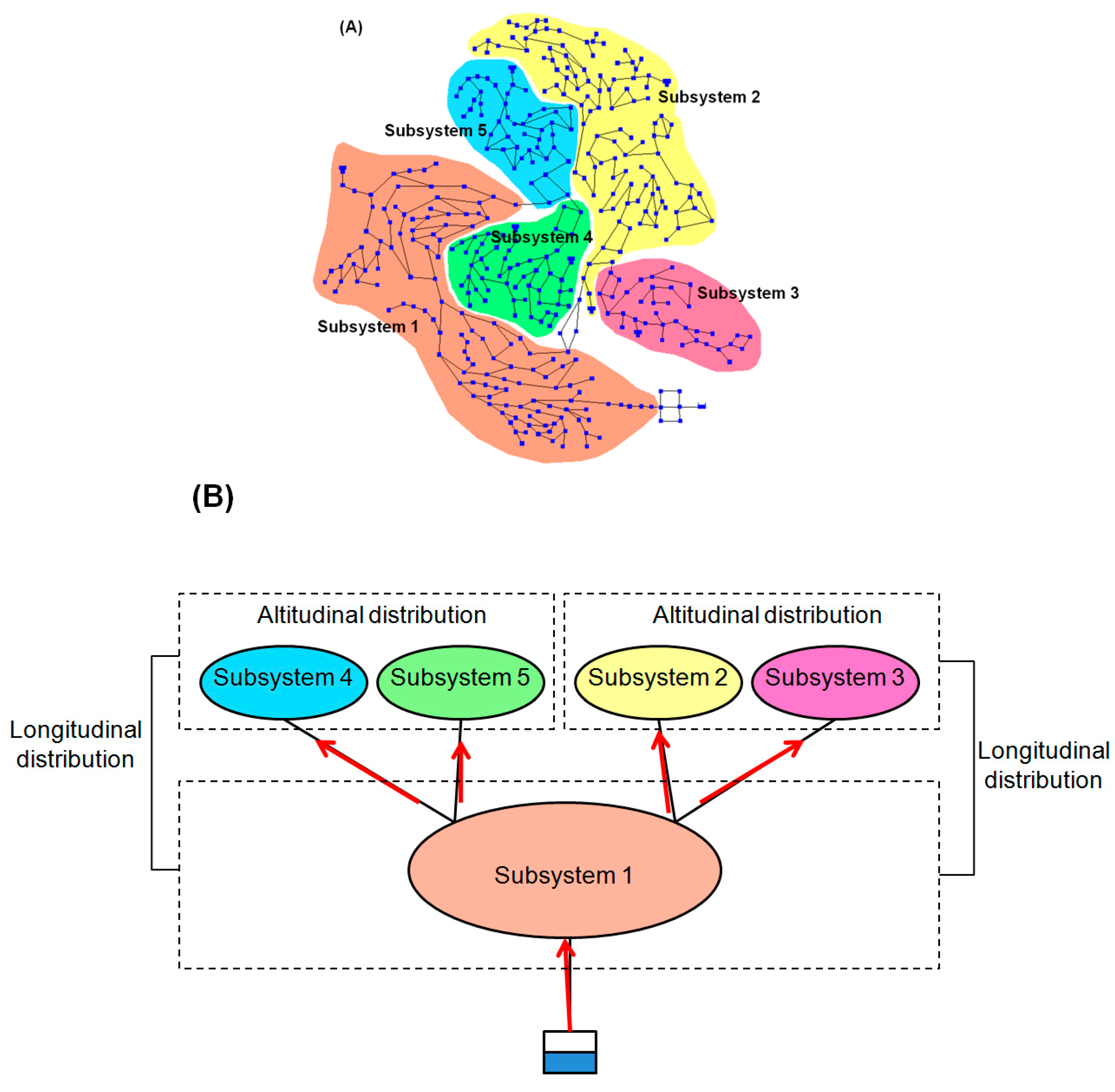
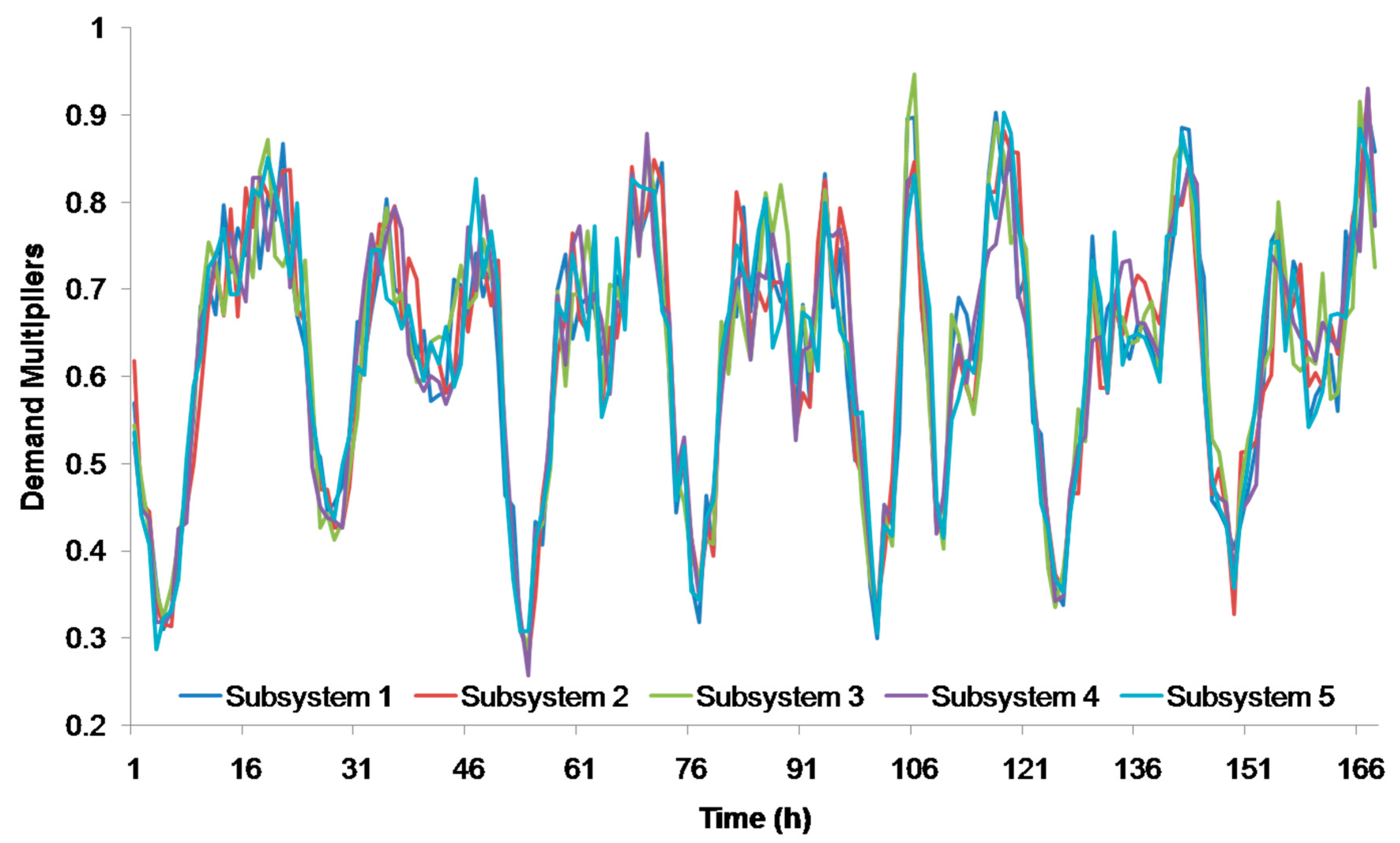
The second case study concentrates on the battle of the water calibration network [17]. The network, known as C-Town, is a benchmark system being comprised of five communities. In each community, pump stations and regulating structures (tanks) are configured. The network topology, including 396 vertices and 444 edges in total, was extracted from the C-Town GIS system (Figure 7A). There is both longitudinal (between community 1 and the other communities) and altitudinal distribution (between community 2 and 3; and between community 4 and 5) in the system, seen in Figure 7B. Estimated monthly water demands are available at each junction, and a unique hourly demand pattern is available for each community for a period of 168 h (Figure 8). The energy tariff is provided in

Table 2. Electricity tariff (€/kWh) used for case study two [18].

Hours in a Day	Monday	Tuesday	Wednesday	Thursday	Friday	Saturday	Sunday
0–6	0.0672	0.0672	0.0672	0.0672	0.0672	0.0672	0.0672
7–9	0.1094	0.1094	0.1094	0.1094	0.1094	0.1094	0.1094
10–16	0.2768	0.2768	0.2768	0.2768	0.2768	0.1094	0.0672
17–19	0.1094	0.1094	0.1094	0.1094	0.1094	0.1094	0.1094
20	0.1094	0.1094	0.1094	0.1094	0.1094	0.0672	0.1094
21–23	0.0672	0.0672	0.0672	0.0672	0.0672	0.0672	0.0672

where the energy prices are shown in cents/kWh. In accordance with case study one, the network is auto-designed using either uniform distributed patterns (weighted average of all given patterns, using monthly demands of communities as weights) or spatial distributed patterns (all patterns are available in Figure 8). Again, the same constraints are imposed on pressure (H ≥ 20 m (196 kPa)) and velocity (0.1 m/s ≤ V ≤ 10 m/s.) respectively for both cases. Thereafter, the impacts are evaluated in the same way as in case study one. For all analyses, the simulation period is 168 h.

4. Results and Discussions

4.1. Case Study One

For the virtual network with altitudinal demand distribution, as

Table 3. Comparisons on diameter distributions and costs of pipe lines (case study one: altitudinal demand distribution).

Diameter (mm)	Pipe Price (€/m)	Total Length (m)			Total Price (€)
		Uniform	Distributed		Uniform	Distributed
			Ideal	Worst		Ideal	Worst
80	33	14,460	13,620	13,460	477,180	449,460	444,180
100	38	3440	3650	3650	130,720	138,700	138,700
150	55	3410	4390	3620	187,550	241,450	199,100
200	75	1920	1570	2040	144,000	117,750	153,000
250	95	1500	1500	460	142,500	142,500	43,700
300	115	570	570	2070	65,550	65,550	238,050
400	175	720	920	720	126,000	161,000	126,000
500	230	310	870	200	71,300	200,100	46,000
600	300	5440	4680	5550	1,632,000	1,404,000	1,665,000
∑ (Capital)					2,976,800	2,920,510	3,053,730

shows, capital cost saving is achieved for the ideal distribution, of which big customers are close to the water source. In this case, the capital cost of distributed design under an ideal pattern (€2,920,510) is about 1.9% cheaper than that of the “Uniform” design (€2,976,800). On the other extreme, the distributed design under the worst pattern requires an expense of €3,053,730 to deliver large amounts of water remotely. Considering the small size of the network and the small differences within the demand patterns (C1–C3), the resulted capital cost difference (i.e., €133,220, about 4.4% higher than the case of ideal pattern) is actually quite considerable. For the virtual network with longitudinal demand distribution, there are marginal differences (about 0.45%) in capital costs of the Uniform and Distributed design (

Table 4. Comparisons on diameter distributions and costs of pipe lines (case study one: longitudinal demand distribution).

Diameter (mm)	Pipe Price (€/m)	Total Length (m)		Total Price (€)
		Uniform	Distributed	Uniform	Distributed
80	33	16,500	15,360	544,500	506,880
100	38	1380	3030	52,440	115,140
150	55	6960	5690	382,800	312,950
200	75	1050	1810	78,750	135,750
250	95	1080	1290	102,600	122,550
300	115	3870	3660	445,050	420,900
400	175	930	930	162,750	162,750
500	230	-	-	-	-
600	300	-	-	-	-
∑ (Capital)				1,768,890	1,776,920

). However, similar to the altitudinal cases, when the network “Uniform” operates under spatial distributed patterns, it may fail to accommodate the peak demand at a certain time step as insufficient pressures (e.g., 21.43 m < 26 m) are witnessed. These results indicate that the spatial distribution of demands for WDSs is to be considered in detail at the design stage to reduce the capital cost and eliminate local pressure problems.

To reflect water quality, the system-wide average water age is computed by summing up the maximum water age of all nodes and subsequently dividing the sum by the number of nodes. As

Table 5. Comparison of water age (case study one).

Longitudinal Demand Distribution		Avg. Water Age (h)	Pump Operating Cost (€/day)
Uniform distributed patterns		0.49	966.56
Spatial distributed patterns		0.50	925.67
Altitudinal Demand Distribution		Avg. Water Age (h)	Pump Operating Cost (€/day)
Uniform distributed patterns		1.41	917.19
Spatial distributed patterns	Ideal demand pattern	1.52	925.67
	Worst demand pattern	1.30	925.67

demonstrates, if a WDS is designed using a uniform pattern, unexpected deterioration problems may occur in reality (i.e., under spatial distributed pattern). However, the “Distributed” design may not ultimately solve this problem, as it leads to increased periods of low flow with a prolonged water retention time in the system.

As for energy consumption, the network “Uniform” and “Distributed” have almost the same pump operating costs in the altitudinal case. Although the uniform distributed patterns triggers slightly lower pump operation costs (less than about 0.93% on average), this is because the average demand of “Distributed” design is a bit larger (about 0.84%) on average due to the unavoidable loss of accuracy during creation of new patterns. Additionally, even though the layouts are different, both the network “Uniform” and “Distributed” have the same energy costs under identical spatial distribution of demand patterns. These results bear out hypothesis 2; i.e., for the same average demand, there might be no crucial differences in energy consumption between the “Uniform” and “Distributed” system. However, in the longitudinal case, the pump operating cost of “Distributed” is about 4% lower than the “Uniform”, which is non-marginal. The reason behind this fact needs further investigation in the future. Nevertheless, both the network “Uniform” and “Distributed” also have nearly identical energy costs under identical spatial distribution of demand patterns.

4.2. Case Study Two

Similar to case study one, the network “Distributed” reduces the capital cost by 93,400 (€) (about 1.6%, calculated based on

Table 6. Comparisons on diameter distributions and costs of pipe lines (case study two).

Diameter (mm)	Pipe Price (€/m)	Total Length (m)		Total Price (€)
		Uniform	Distributed	Uniform	Distributed
80	33	8065.03	8674.24	266,145.99	286,249.92
100	38	8445.86	9814.95	320,942.68	372,968.10
150	55	9340.02	8790.09	513,701.10	483,454.95
200	75	6312.52	8084.55	473,439.00	606,341.25
250	95	7165.84	4324.53	680,754.80	410,830.35
300	115	4120.08	4584.01	473,809.20	527,161.15
400	175	5535.40	3867.74	968,695.00	676,854.50
500	230	4014.88	4203.06	923,422.40	966,703.80
600	300	3724.14	4380.60	1,117,242.00	1,314,180.00
∑ (Capital)				5,738,152.17	5,644,744.02

). Table 6 summarizes the diameter distributions and costs of pipes with different diameters in the two auto-designed networks. The difference between the two cases is not remarkable, as there appears to be little difference between the demand patterns. This effect is more pronounced in large scale systems with significant variant demand patterns. As the average of maximum water age hours increases by a maximum of 7.45 h (

Table 7. Comparison of water age (case study two).

Network “Uniform”	Avg. Water Age (h)	Pump Operating Cost (€/day)
Uniform distributed patterns	33.74	711.78
Network “Distributed”	Avg. Water age (h)	Pump operating cost (€/day)
Spatial distributed patterns	40.37	697.50

), water quality is diminished for the network “Distributed”. Considering energy cost, there are rather small differences coming from the same reason as discussed in the “Case Study One” section. This study further confirms that, for a specific WDS, the spatial distribution of demand could have non-negligible effects on capital cost, water age, and energy consumption.

5. Conclusions

Water distribution systems (WDSs) are typically designed using a uniform demand pattern, whereas there might be noteworthy differences among regional-specific demand patterns. As a result, a WDS may fail to provide an expected level of services when it is running under the unexpected real demand patterns. Constrained by data availability and resolution of data, it may not always be feasible to fully understand the spatial distribution of demand patterns and the corresponding effects. Despite estimation, spatial variability is a difficult job. However, regarding the design under uncertainty, this study provides insight on if it is worthwhile to further focus on spatial variability in the design process or not, or if other sources of uncertainty (e.g., demand itself) are more important.

This study shows that the layouts/configurations play a decisive role, and the impact of the spatial distributed patterns is rather crucial. The analysis of the spatial variability of demand patterns allows to conclude for water distribution system design and operation as follows:

• Water distribution system design based on spatial distributed demand patterns may reduce capital cost (e.g., about 4.4%) in systems in which communities with high peak demands are close to the water source and vice versa. For practical application, an uncertainty analysis can be made to compare the cost efficiency and performance of a number of designs based on different possible demand patterns. Further, the cost efficiency analysis should evaluate the saving on capital cost as well as any extra investments required for addressing the demand spatial variability by detailed demand assessment.
• As for water age, the spatial distribution of demand induces water age deterioration. For example, the average water retention time is prolonged by 7.45 h in case study two under spatial-variant patterns. This phenomenon mainly results from the appearance of increased periods of low flow—particularly in communities with a high peaking factor.
• Irrespective of the demand patterns used in the design phase, the pump operating costs are nearly identical in all cases as long as the same average demands are applied.

As a result, it is important to check the system’s performance using community-specific demand patterns at the design stage. The “Uniform” design strategy might result in higher life-cycle cost (with similar operational cost, but higher capital cost), and failures to meet pressure constraints during peak times.

As a next step, not only the effect of more complex demand patterns should be investigated, but also the effect of temporal variability (by using historical water demand records). The results, accounting for both spatial and temporal variability, would further improve engineering decision making both in design strategy and operational control.

References

- Butler, D.; Ward, S.; Sweetapple, C.; Astaraie-Imani, M.; Diao, K.; Farmani, R.; Fu, G. Reliable, resilient and sustainable water management: the Safe & SuRe approach. Glob. Chall. 2016. [Google Scholar] [CrossRef]
- Gora, S. Executive Summary. In Study on Water Quality and Demand on Public Water Supplies with Variable Flow Regimes and Water Demand; CBCL Limited: Halifax, NS, Canada, 2011. [Google Scholar]
- Preis, A.; Allen, M.; Whittle, A.J. On-Line Hydraulic Modeling of a Water Distribution System in Singapore. In Proceedings of the Water Distribution System Analysis 2010–WDSA2010, Tucson, AZ, USA, 12–15 September 2010. [Google Scholar]
- Filion, Y. Impact of Urban Form on Energy Use in Water Distribution Systems. J. Infrastruct. Syst. 2008, 14, 337–346. [Google Scholar] [CrossRef]
- Sitzenfrei, R.; Möderl, M.; Mair, M.; Rauch, W. Modeling Dynamic Expansion of Water Distribution Systems for New Urban Developments. In Proceedings of the World Environmental and Water Resources Congress 2012, Albuquerque, NM, USA, 20–24 May 2012; pp. 3186–3196. [Google Scholar]
- Diao, K.G.; Zhou, Y.W.; Rauch, W. Automated creation of district metered areas boundaries in water distribution systems. J. Water Res. Plan. Man. 2012, 139, 184–190. [Google Scholar] [CrossRef]
- Kanakoudis, V.; Gonelas, K. Accurate water demand spatial allocation for water networks modelling using a new approach. Urban Water J. 2015, 12, 362–379. [Google Scholar] [CrossRef]
- Filion, Y.; Adams, B.; Karney, B. Cross Correlation of Demands in Water Distribution Network Design. J. Water Res. Plan. Man. 2007, 133, 137–144. [Google Scholar] [CrossRef]
- Diao, K.G.; Barjenbruch, M.; Bracklow, U. Study on the Impacts of Peaking Factors on a Water Distribution System in Germany. Water Sci. Technol. Water Supply 2010, 10, 165–172. [Google Scholar] [CrossRef]
- Sitzenfrei, R.; Möderl, M.; Hellbach, C.; Rauch, W. Application of a Stochastic Test Case Generation for Water Distribution Systems. In Proceedings of the World Environmental and Water Resources Congress 2011, Palm Springs, CA, USA, 22–26 May 2011; pp. 113–120. [Google Scholar]
- Muranho, J.; Ferreira, A.; Sousa, J.; Gomes, A.; Sá Marques, A. WaterNetGen: an EPANET extension for automatic water distribution networks models generation and pipe sizing. Water Sci. Technol. Water Supply 2012, 12, 117–123. [Google Scholar] [CrossRef]
- Rossman, L.A. EPANET 2 Users Manual; U.S. Environmental Protection Agency: Cincinnati, OH, USA, 2000.
- Kirkpatrick, S.; Gelatt, C.D.; Vecchi, M.P. Optimization by Simulated Annealing. Science 1983, 220, 671–680. [Google Scholar] [CrossRef] [PubMed] [Green Version]
- Cunha, M.C.; Sousa, J. Hydraulic infrastructures design using simulated annealing. J. Infrastruct. Syst. 2001, 7, 32–39. [Google Scholar] [CrossRef]
- Cunha, M.C.; Sousa, J. Water distribution network design optimization: Simulated annealing approach. J. Water Res. Plan. Manag. 1999, 125, 215–221. [Google Scholar] [CrossRef]
- Walski, T.M.; Chase, D.V.; Savic, D.A.; Grayman, W.; Beckwith, S.; Koelle, E. Chapter 4.2 Peaking factors. In Advanced Water Distribution Modeling and Management, 1st ed.; Haestad Press: Waterbury, CT, USA, 2003; Volume 154. [Google Scholar]
- Ostfeld, A.; Salomons, E.; Ormsbee, L.; Uber, J.G.; Bros, C.M.; Kalungi, P.; Burd, R.; Zazula-Coetzee, B.; Belrain, T.; Kang, D.; et al. The Battle of the Water Calibration Networks (BWCN). J. Water Res. Plan. Manag. ASCE 2011, 138, 523–532. [Google Scholar] [CrossRef]
- Salomons, E.; Ostfeld, A.; Kapelan, Z.; Zecchin, A.; Marchi, A.; Simpson, A.R. Detailed Problem Description and Rules. The Battle of the Water Networks II–Adelaide 2012 (BWN-II). In Proceedings of the Water Distribution Systems Analysis Conference 2012, Adelaide, Australia, 24–27 September 2012; Available online: http://wdsa2012.com/ (accessed on 14 February 2012).
Figure 1.
The possible differences between the design demand pattern (uniform distributed patterns) and real demand patterns (spatial distributed patterns).
Figure 2.
Spatial distribution of demands. (A) altitudinal distribution; (B)longitudinal distribution.
Figure 3.
An example of the ideal altitudinal demand distribution. (A) system capacities estimated based on uniform distributed patterns; (B) system capacities estimated based on spatial distributed patterns.
Figure 4.
Creation of spatial distributed demand patterns based on system decomposition.
Figure 5.
The creation and design patterns of the case study one networks. (A) the altitudinal distribution; (B) the longitudinal distribution.
Figure 6.
The three demand patterns used in case study one.
Figure 7.
The case study two network. (A) the layout and demand partition; (B) the spatial distribution of demand.
Figure 8.
Demand pattern of each subsystem in the case study two network.