Article

Dominant Hydro-Climatic Drivers of Water Temperature, Salinity, and Flow Variability for the Large-Scale System of the Baltic Coastal Wetlands

1
Department of Sustainable Development, Environmental Science and Engineering, Royal Institute of Technology (KTH), 100 44 Stockholm, Sweden
2
Department of Physical Geography, Bolin Centre for Climate Research, Stockholm University, 106 91 Stockholm, Sweden
*
Author to whom correspondence should be addressed.
Water 2019, 11(3), 552; https://doi.org/10.3390/w11030552
Submission received: 16 January 2019 / Revised: 20 February 2019 / Accepted: 11 March 2019 / Published: 17 March 2019

Abstract

:
For the large-scale coastal wetland system of the Baltic Sea, this study develops a methodology for investigating if and to what degree the variability and changes in certain hydro-climatic drivers control key coastal–marine physical conditions. The studied physical conditions include: (a) water temperature, (b) water salinity, and (c) flow structures (magnitudes and directions of flows between marine basins and the associated coastal zones and wetlands). We use numerical simulations of three hydro-climatically distinct cases to investigate the variations in hydro-climatic drivers and the resulting physical conditions (a–c) among the cases. The studied hydro-climatic forcing variables are: net surface heat flux, wind conditions, saltwater influx from the North Sea, and freshwater runoff from land. For these variables, the available observation-based data show that the total runoff from land is significantly and positively correlated with precipitation on the sea itself, and negatively correlated with saltwater influx from the North Sea to the Baltic Sea. Overall, the physical condition (a–c) variability in the Baltic Sea and its coastal zones is found to be pairwise well-explained by simulation case differences as follows: (a) Net heat flux is a main control of sea water temperature. (b) Runoff from land, along with the correlated salt water influx from the North Sea, controls average sea salinity; with the variability of local river discharges shifting some coastal zones to deviate from the average sea condition. (c) Wind variability and change control the Baltic Sea flow structure, primarily in terms of flow magnitude and less so in terms of flow direction. For specific coastal wetland zones, considerable salinity differences from average Baltic Sea conditions (due to variability in local river discharges) are found for the coasts of Finland and Estonia, while the coastal wetland zones of south-eastern Sweden, and of Estonia and Latvia, emerge as particularly sensitive to wind shifts.

1. Introduction

Unique areas of extensive and ecologically diverse boreal coastal wetlands are distributed along the coastline of the Baltic Sea [1,2], one of the world’s largest brackish water bodies, with a land catchment area that is about four times greater than the sea surface area [3] (Figure 1). The Baltic coastal wetlands experience small tidal variations, and they are subject to irregular flooding, due to their generally low elevation relative to mean sea level, and their associated low seaward gradients [2]. As such, sea level changes in the Baltic are essential for the hydro-geography and ecology of its coastal zones and wetlands, and have been determined by the net balance of postglacial isostatic rebound of land, and the global eustatic sea level rise (SLR) due to the global warming phenomenon, in combination with the water balance of the Baltic Sea itself [4].
From the balance between isostatic land rebound and climate-driven SLR, the approximate equilibrium position of zero net sea level change in the Baltic has been reported by [5] to fall somewhere through the marine basin of the Northern Baltic Proper (NBP) for the estimated average current SLR rate of around 3 mm/year [6] (dotted purple line in Figure 1b). The equilibrium position for potential future higher SLR rates is estimated to move northward to around the northern border of the NBP at a rate of 4 mm/year, and the northern borders of Åland Sea and Archipelago Sea, at a rate of 5 mm/year (dashed and solid purple lines, respectively, Figure 1).
So far, net sea level changes have been mostly driven by the development/emergence of coastal wetlands in the Baltic, with variations in atmospheric pressure and storm surges being reported to also considerably contribute an additional sedimentary component to this development, for areas around the estimated current equilibrium line [2]. However, potential future acceleration in the rate of the climate-driven SLR may alter this relationship, and may further enhance and move northward the problem of shore erosion, which is already being experienced in areas south of the current average equilibrium line [8]. Accelerated SLR will particularly affect Baltic coastal wetlands with limited allochthonous sediment supplies [9], and the favorable combinations of micro-topographic, hydrological, and sea-level conditions [10].
Besides these relatively well-investigated effects of sea level changes [2,9,10], there are also additional weather/climate variabilities and change aspects that may affect coastal wetlands, including those in the Baltic coast [5]. From a recent review of wetland-related research, hydro-climatic variability and change emerge as the expected key change drivers for most wetland functions, but with large identified research gaps regarding wetland impacts, in particular for the large-scale dynamics of systems with multiple wetlands, and mostly so for coastal wetland systems [11]. For the Baltic Sea, investigations that are focused on coastal wetlands have mainly addressed sea level rises. However, coastal wetlands that are connected to the sea are also affected by changes in sea temperature and salinity, as well as by currents, for which research is still limited [11].
Previous studies have investigated the variability of Baltic Sea physical conditions (e.g., Lehmann and Hinrichsen [12] studied fluxes among marine basins, finding high inter- and intra-annual variability), and they have also proposed some relationships between hydro-climatic forcing and physical conditions [13,14]. The aforementioned studies have focused on either a certain type of hydro-climatic driver (e.g., meteorological forcing [13]), or a certain physical condition (e.g., salinity [14]), or on only parts of the Baltic Sea (e.g., Arkona Basin, Bornholm Channel and Stope Channel of the Baltic Sea [12]). Comprehensive understanding of the integrated effects of multiple forcings on multiple physical variables in the sea is still lacking. In this paper, we expand upon earlier studies, and we consider multiple landscape, atmospheric, and sea forcings, to improve our overarching understanding, and to envelope the inherent correlations and joint effects of these forcings on different physical conditions in the large-scale Baltic Sea system and its coastal wetland zones.
Specifically, variability, change, and correlations between various hydro-climatic conditions, and their impacts on the following physical coastal–sea conditions are investigated: (a) water temperature, (b) salinity, and (c) flow structure (magnitudes and directions of flows between different marine basins and coastal zones). These physical conditions are fundamental for the hydrodynamics as well as the water quality and eutrophication of the Baltic Sea and its coastal waters [15], and for the associated occurrences of harmful algae blooms, hypoxic areas, and dead zones [16,17].
In order to investigate how the physical coastal–sea conditions (a–c) are affected by hydro-climates in terms of hydrological and sea-related weather/climate variabilities and changes in the Baltic region, we hypothesize that some predominant cause–effect pathways of determination may emerge for these conditions, by primarily focusing on the following main forcing variables: (i) net surface heat flux, and (ii) wind conditions over the Baltic Sea; (iii) saltwater flux from the North Sea into the Baltic Sea; and (iv) freshwater discharges (runoff) from land into the Baltic Sea. These are general main forcing variables in ocean modeling [18], and these relate to physical sea conditions that are also in the Baltic Sea [12,13,14]. To test this hypothesis, we consider and use hydrodynamic simulations with the open-source three-dimensional model, the “Finite-Volume, Primitive Equation Community Ocean Model” (FVCOM) [18]. Available observation-based data for the forcing variables (i–iv) for different years are used to determine and drive three hydro-climatically distinct simulation cases. By comparing the simulation results for these three cases, we test and analyze if and to what degree the variability and change in the hydro-climatic forcing variables (i–iv) control the resulting physical conditions (a–c) in the Baltic Sea, and in its coastal zones and wetlands.

2. Materials and Methods
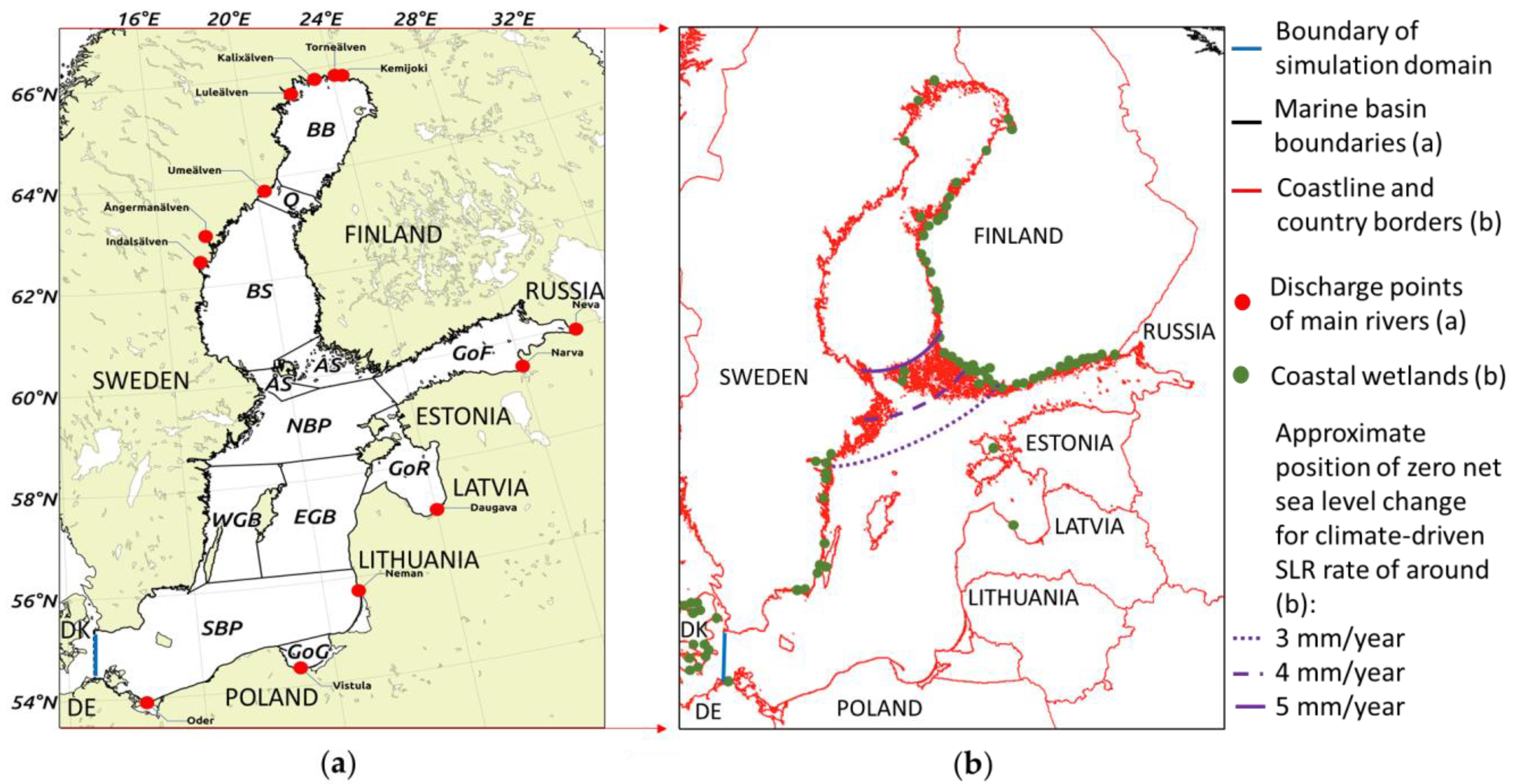
This study aims at identifying main driver–effect relationships for the Baltic Sea, and its coastal zones and wetlands (Figure 1), by analyzing FVCOM simulation results for three hydro-climatically distinct cases (Table 1). The analysis considers the targeted physical coastal–marine conditions (a–c above) and their dependence on the different forcing variable sets (i–iv above) in these cases, which are described further in Table 1 and its title, and in the simulation approach in Section 2.4 below.

2.1. The Baltic Sea

The Baltic Sea is a brackish water system in northern Europe, extending between 10° E and 30° E longitude, and between 53° N and 66° N latitude (Figure 1). This is an important coastal–marine water environment for the nine countries within the total Baltic Sea catchment area of 1,739,400 km2 [3]. From this catchment, the Baltic Sea receives a total freshwater discharge of around 480 km3/year; this total discharge also carries with it considerable waterborne nutrient loads [19] that depend greatly on the discharge magnitude [20] and its hydro-climatically determined variability and change [21]. Furthermore, the Baltic Sea has a relatively small exchange of sea water through its narrow connection with the North Sea at the Danish Straits [22]. This small exchange makes the physical conditions and the water quality in the Baltic Sea and its coastal zones and wetlands particularly sensitive to freshwater discharges and waterborne nutrient loads from land. In addition, the physical and water quality conditions in the coastal zones and their wetlands also depend greatly on marine conditions and their interactions with coastal waters [15].

2.2. Data

Observation data for water level, salinity, and temperature in the Baltic Sea were obtained for different sea measurement stations from the Swedish Meteorological and Hydrological Institute (SMHI) [23,24]. Data for yearly total freshwater discharges to the coast were obtained from the Baltic Marine Environment Protection Commission—Helsinki Commission (HELCOM) [25]. Noting that the seven largest Baltic rivers contribute nearly half of the total discharge to the sea [19], we considered in our model simulations discharges from the 13 largest rivers, based on the data availability and major discharge contributions of these rivers in the validation year of 2005 (see further description Supplementary Material (SM) Part A); the 2005 discharge contributions are consistent with the corresponding long-term discharge contributions of these rivers [26,27]. At any rate, some cutoff choice needs to be made for the number of rivers to be considered in the simulations, because the relevant time series of river discharge data are not openly accessible and cannot be readily constructed for all Baltic rivers, and the 13 selected rivers account for around 65% of the total river discharge into the present Baltic Sea simulation domain (Figure 1).
The available time series of daily discharge data for most of the 13 rivers were obtained from SMHI [28] and the Global Runoff Data Centre (GRDC) [29]. For the rivers Narva, Daugava, Oder, and Vistula, we did not have access to openly available data from official agencies for their daily discharges to the Baltic Sea. For these rivers, we constructed the required discharge time series by the use of available data for their respective long-term average annual discharges [30], and by assuming similar daily and inter-annual discharge variations around the respective long-term average discharge of each river with the available daily data, except Neva. Neva was excluded from this calibration averaging, because it has a different wet–dry pattern than the other considered rivers; for example, Neva is predominantly responsible for wetter than average conditions in one of the three representative hydro-climatic years (2005, “R+,T--” case, Table 1).
Wind data were extracted from the ERA20 reanalysis model of the European Centre for Medium-Range Weather Forecasts (ECMWF) [31]. Heat flux data were obtained as the combined products of the Objectively Analyzed Air–Sea Fluxes for the Global Oceans Project from Woods Hole Oceanographic Institution (WHOI OAFlux project) [32] and the International Satellite Cloud Climatology Project (ISCCP) [33]. Precipitation and air temperature data were obtained from SMHI [34], based on meteorological observations.

2.3. The Model FVCOM

The three-dimensional model FVCOM [18] was used to simulate Baltic Sea conditions, with a focus on the targeted physical coastal–sea conditions (a–c). The model is based on the primitive equations of momentum to simulate free-surface water motion, and it uses the Mellor and Yamada level 2.5 (MY-2.5) turbulent closure model [35] to calculate turbulence [18]. Furthermore, it uses the finite volume method for discretization, leading to good mass conservation. In the model, an unstructured triangular grid is used horizontally, and sigma layers are used in the vertical direction, which are typically used for good representations of water bodies with complicated coastlines and bathymetry. The FVCOM model has been verified over a wide range of cases for coastal and ocean water modeling (for example, the Arctic Ocean, by Chen et al. [36]; the Gulf of Maine and the New England Shelf, UK, by Chen et al. [37]; Scituate Harbour, USA by Beardsley et al. [38]; extensive marine domains including the entire South China Sea, the entire Indonesian archipelago, part of the western Pacific, and eastern Indian oceans, by Wei et al. [39]).
The Baltic Sea FVCOM model was set up with a 10 km horizontal resolution for the triangular grid, and the vertical depth was divided into 20 uniform layers. In our simulations, the connection to the North Sea was set through the boundary at Skanör (blue boundary line, Figure 1a,b). The model was driven by the forcing variables (i–iv) and some additional required and available input data (such as the water level and water temperature for the open boundary to the North Sea). The model was validated against observed temperature, salinity, and water elevation data with settings for the year 2005. More details on the model setup, as well as the validation results, are given in Part A of SM.

2.4. Simulation Approach

The basic FVCOM model setup for the Baltic Sea simulations used independently available data time series as inputs for the forcing variables, and the model results from this setup simulation were validated against the independently available data for the targeted physical conditions (a–c) in 2005 (see further descriptions of the model setup and the validation process in SM Part A, and further data descriptions in Section 2.2). The validation shows that this model setup can sufficiently reproduce the Baltic Sea annual water temperature circle, the salinity distribution pattern both horizontally and vertically, and the overall circulation pattern (SM Part A). For the main comparative simulation aim of this study, the three hydro-climatically distinct cases (Table 1) were chosen for further stylized comparative simulations, representative of realistic variability in the investigated hydro-climatic forcing sets (i–iv), based on the actual differences seen in the relevant characteristic data for the years 2005, 2000, and 2003.
The three hydro-climatically different simulation cases represent (Table 1): a wet and relatively cold case ’’R+,T--” (based the characteristics for 2005), a wet and particularly warm case “R+,T++” (based on the characteristics for 2000), and a particularly dry and relatively warm case “R--,T+” (based on the characteristics for 2003). We defined the cases with different degrees of wet/dry and warm/cold conditions by comparing their river discharges and net heat fluxes of the selected case years, with the corresponding 10-year average values over 2000–2009. Values smaller than the average are referred to as being drier/colder; values larger than average are referred to as wetter/warmer. Values that are two standard deviations larger or smaller than average are referred to as being particularly warm or particularly dry. We chose the representative years from the period 2000- 2009, because the data for all required forcing variables are available for this period. According to available data for river discharges into the Baltic Sea over the longer period 1952–2012 [25], the year of 2003 was the driest year of all in that longer period, while the year of 2000 was the sixth wettest year (the wettest in the period of 2000–2009). The year of 2005 is a normal year when considering the total discharges into the sea, while it is wetter than average when considering only the 13 largest rivers (as Neva was significantly wetter in that year). Considering the possible regional changes towards wetter and warmer climates, the year of 2000 may be representative of such conditions, while 2003 may be representative of possible drier future summer conditions.
For direct result comparability, the simulations of these hydro-climatic cases started from the same initial conditions. These were obtained from the results of a one-year simulation, with the initialization and hydro-climatic settings of the relatively wet and cold case, “R+,T--” (based on 2005). In each simulation case, the forcing set included the associated: (i) net heat flux and (ii) wind conditions in the sea, (iii) saltwater flux from the North Sea, and (iv) freshwater discharges from the land.
The forcing variables (i–iv) differed among the cases, as they differed among the three years that these cases were based on (Table 1). In the simulation of each case, the associated forcing set was repeated until an equilibrium quasi-steady state was reached (with intra-annual/seasonal variations around the stable long-term average result values). The simulations continued for as many simulation years as needed, to reach this equilibrium quasi-steady state for the targeted physical Baltic Sea conditions: (a) water temperature, (b) salinity, and (c) flow structure. The different case simulations were finally compared in terms of these robust equilibrium results, with the aim to investigate if and to what degree the forcing variables (i–iv) were dominant in driving the physical conditions (a–c) toward the different case results for the Baltic Sea and its coastal wetland zones.

3. Results and Discussion

3.1. Data-Given Correlations among the Hydro-Climatic Forcing Variables

As a basis for interpreting the relationships between forcing variables (i–iv) and physical conditions (a–c), we first investigated statistically, based on the available data, whether some of the forcing variables (i–iv) are mutually correlated. The total yearly river discharge (or, by catchment area normalization, the runoff R) to the Baltic Sea [25] was used as a main comparative variable, to quantify the hydrological wetness or dryness of each hydro-climatic case. We thus investigated the correlation between the case wetness/dryness in terms of R and the other forcing variables, as outlined in Table 2.
In our model of the Baltic Sea, precipitation was assumed to be more or less balanced by evaporation. In other words, the net effect of precipitation minus evaporation was neglected because this difference is much smaller than the river discharges, and as such, it is less important for the Baltic net outflow [13]. Nevertheless, precipitation is an important hydro-climatic variable, and it was considered in Table 2 with regard to its correlation with other hydro-climatic variables for the Baltic Sea. Precipitation over the sea was then found to be significantly and positively correlated with total R into the sea. Precipitation and R were thus consistent in representing the relative wetness/dryness of a simulation case. Furthermore, the measured salinity at the open boundary to the North Sea (measurement station called By1) and an associated salinity inflow index [40] were significantly and negatively correlated with the total R. In contrast, neither the heat flux (or the associated air temperature), nor the wind-forcing variables were significantly correlated with R.
The results of previous studies have shown wind conditions to be correlated with saltwater inflow from the North Sea to the Baltic Sea [41,42]. The identification of such possible correlations also in the periods with available data for our investigation (Table 2) may require data analysis with finer temporal resolution [41] than the annual resolution underlying the present results (Table 2). However, such fine resolution is not essential for the main aim of our study to investigate the possible dominant relationships between some typical annual forcing characteristics and resulting average physical conditions in the Baltic Sea. The data-given correlation results (Table 2) imply that in wet (dry) years, as represented by the simulation cases “R+,T--”, “R+,T++” (“R--,T+”), the saltwater influx from the North Sea to the Baltic Sea and its coastal zones and wetlands are smaller (greater) than average. In the following section, we further discuss the simulated effects of the main forcing variables (i–iv) on the physical conditions (a–c).

3.2. Simulation Results

3.2.1. Model Validation for the Baltic Sea

The validation of the Baltic Sea model was based on the year of 2005, as this is a hydrologically normal year according to available data on total river discharge into the Baltic Sea. The model was validated against the observed data for temperature, salinity, and water level. The annual average flow field is also compared with the simulation results from previous research [43,44], with further validation details shown in SM Part A.
In summary, observed and simulated water salinity and temperature as functions of time and depth were compared at observation stations C3, By31, and By15 over the Baltic Sea. The observed and simulated water level time series were compared at Oskarshamn Station and Skagsudde Station (the station locations are shown in SM, Figure S2). The simulated water salinity, temperature and water level are all consistent with the observed values, indicating the model as capable of reproducing the hydrodynamic processes, including salinity stratification, thermal cycle, and the general circulation of the Baltic Sea.

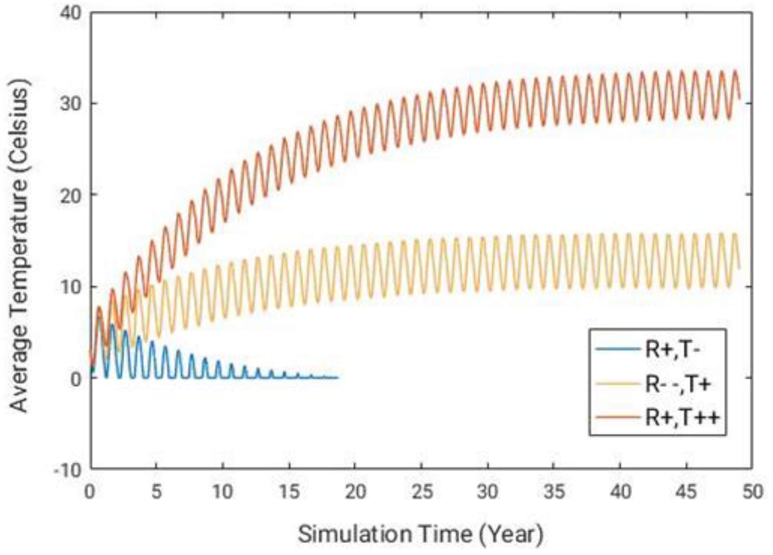
3.2.2. Water Temperature (Physical Condition a)

The average water temperature in the coastal–marine waters of the Baltic Sea at simulated quasi-steady state conditions was generally highest for the particularly warm and wet case “R+,T++”, considerably lower for the warm and particularly dry case “R--,T+”, and the lowest for the cold and wet case “R+,T--” (Figure 2). The simulation time for case “R+,T--” only extended to 6825 days (nearly 19 years) because the average sea temperature reached then 0 °C, and remained at that level for simulation times of beyond 6825 days.
The considerable differences in the resulting water temperature between the case “R+,T++” and the case “R+,T--”, which have similar R and salt water influx conditions, implies a small influence of these forcing variables on sea temperature. Also the resulting mid-range water temperature for the mid-range heat-flux forcing in the case of “R--,T+” (under particularly dry and, by negative correlation (Table 2), high saltwater influx conditions) was consistent with the net heat flux being dominant in driving water temperature differences among the simulation cases.
In the present model, net heat flux rather than air temperature was a driving boundary condition. As these variables are related, air temperature is also part of determining the water temperature, along with the associated heat flux forcing. However, both of these heat-related variables are essentially independent of the wetness/dryness-related variables runoff and precipitation, as well as of the other investigated types of forcing variables (Table 2), which in turn also have small influence on the water temperature condition. As such, the conclusion remains that the net heat flux forcing (along with other variables that this is related with, such as air temperature) is dominant in determining water temperature in comparison to the other investigated forcing variables.

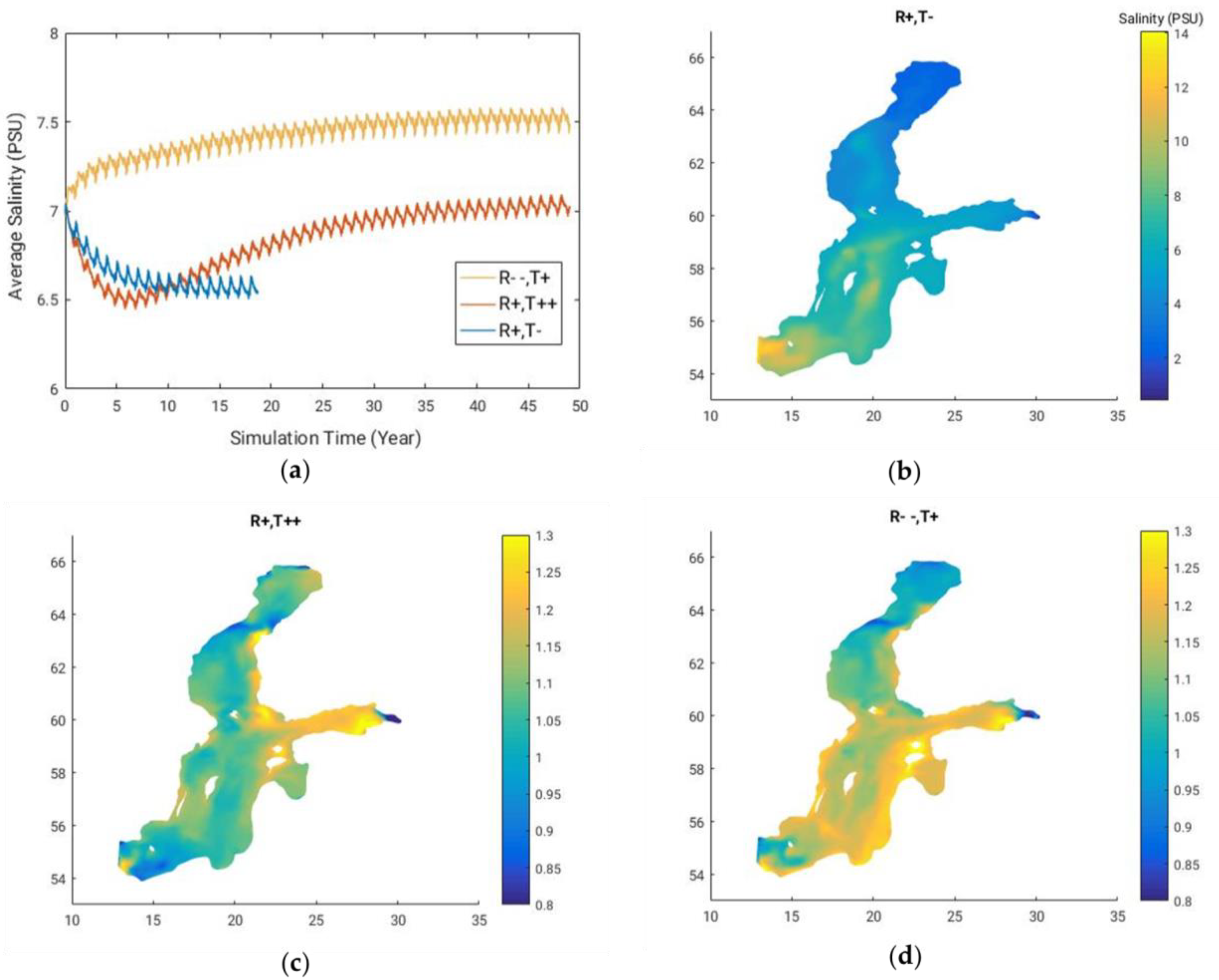
3.2.3. Salinity (Physical Condition b)

The average sea salinity at the simulated quasi-steady state (Figure 3a) was similar between the wet and cold case “R+,T--” (Figure 3b) and the wet and particularly warm case “R+,T++” (Figure 3c). For the eastern coastal wetlands along the coast of Finland and Estonia, however, the salinity was considerably higher in the “R+,T++” than in the “R+,T--” case (Figure 3c); this is because the discharge into the Gulf of Finland from the largest river, Neva, was smaller in case “R+,T++”.
Overall, salinity was highest for the particularly dry and warm case of “R--,T+” (Figure 3d). Comparison of the “R--,T+” case with the other two cases indicates runoff into the sea, and its negative correlation with salinity and saltwater influxes at the open boundary to the North Sea, as major controls of salinity in the open sea and the coastal zones with wetlands.
For comparison with measured salinity conditions at the open boundary to the North Sea (Figure S7, Part B of SM), average vertical salinity at measurement station By1 near this boundary was 10.65 PSU, 9.89 PSU and 9.77 PSU in the years 2003, 2000, and 2005, associated with the cases of “R--,T+”, “R+,T++” and “R+,T--”, respectively. From these salinity data and the correlation and simulation results, we can thus conclude that dry conditions with relatively low freshwater discharge to the sea, as represented by simulation case “R--,T+”, also imply higher salinities at the open sea boundary, and more salt water intrusion from the North Sea. These forcing variables thus combine in leading to the highest salinity for the driest case, “R--,T+”, in both the open sea and the coastal zones and wetlands (Figure 3d).

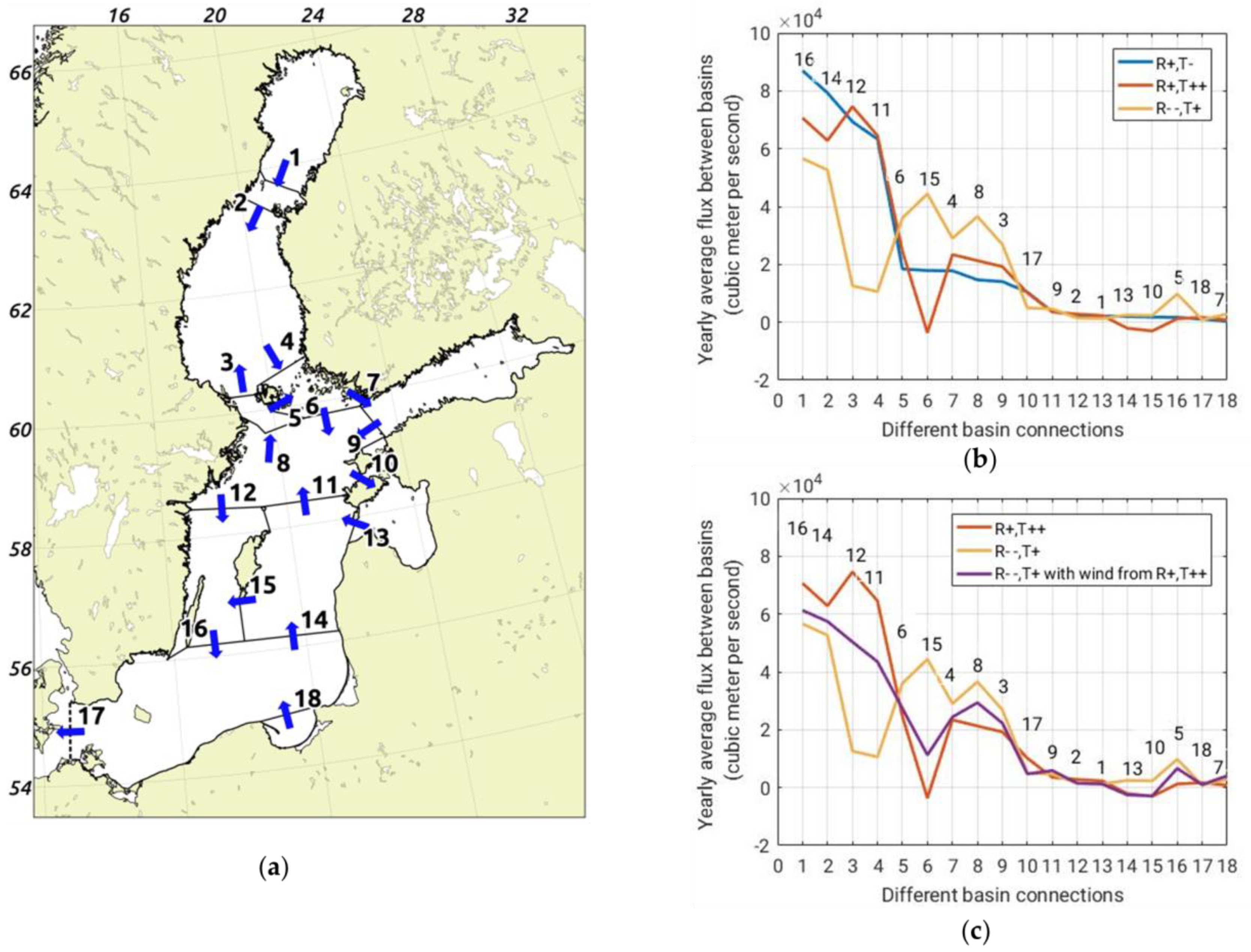
3.2.4. Flow Structure (Physical Condition c)

Flow structure was quantified in terms of the directions and rates of flow among the 12 main marine basins of the Baltic Sea [45] (see basin names and acronyms in Figure 1a). These flows range widely, and they are largest across the NBP, Southern Baltic Proper (SBP), Eastern Gotland Basin (EGB), and Western Gotland Basin (WGB) boundaries (16, 14, 12, 11, 15, and 6 in Figure 4).
The simulation results show that most of these large flows are stable, and they do not change their directions across the cases “R+,T--”, “R+,T++”, and “R--,T+” (Figure 4b, and Figure S9 in Part B of SM), even though the hydro-climatic forcing varied significantly among the cases. The largest simulated flow with changed direction from that shown in Figure 4a (for “R+,T--” as a base case) is that from EGB into WGB (boundary 15, for case “R+,T++”), which may particularly affect the Swedish coastal wetland zone in the WGB. In addition, the relatively small flows into and out from the Gulf of Riga (GoR; boundaries 10 and 13, respectively; see further Figure S9 in Part B of SM) also changed directions in the case of “R+,T++”, which may particularly affect the Estonian and Latvian coastal wetlands.
Overall, the flow structure in the Baltic Sea and along or to/from its coastal wetland zones is more similar for the wet cases “R+,T--” and “R+,T++” than between any of these and the dry case “R--,T+”. Relative to the other two wet cases, the dry case “R--,T+” (yellow in Figure 4b,c) exhibits a large decrease in the magnitude of flow from the NBP into the WGB (boundary 12), and further along the Swedish coastal wetland zone in the latter; for the WGB, this inflow decrease is to some degree compensated by a considerable increase in the magnitude of inflow to the WGB from the EGB (boundary 15). Furthermore, this outflow increase for the EGB, as well as that from the NBP, is in turn compensated by an associated large decrease in the magnitude of outflow from the EGB into the NBP (boundary 11).
In summary, the dry case “R--,T+” implies considerable changes in local circulation that are of relevance for the wetlands along the eastern Swedish coastline in the WGB. However, comparison between Figure 4b,c shows that it is the wind conditions, rather than the wetness (R) conditions, that lead to these circulation changes in this case. Specifically, as an additional test case for examining the role of wind, we also simulated and illustrate in Figure 4c results for the dry case “R--,T+”, but with the wind conditions of case “R+,T++” (see wind conditions for the different cases in Figure S8, Part B of SM). The flow results for the wind-modified dry case “R--,T+” (purple, Figure 4c) differ considerably from those for the original case “R--,T+” (yellow, Figure 4c), and they are more similar to those for the wet case “R+,T++”. Even though the wetness of the latter case has some influence on the flow results, in particular for small basins with direct river discharges into them, this test shows that the prevailing wind field is a main control of flow structure in the Baltic Sea, and particularly so for the WGB, EGB, and NBP basins. This adds to the above-noted effects of wind conditions in the “R+,T++” case for both flow directions and flow magnitudes of relevance for the coastal wetland zone of Sweden in the WGB.

4. Conclusions

For the investigated forcing variables (i–iv), the available data show that total runoff from the land to the Baltic Sea coast is significantly and positively correlated with the precipitation on the sea itself, as well as negatively correlated with the saltwater influx from the North Sea into the Baltic Sea. The main conclusions from the comparative simulation results for the different hydro-climatic cases are: A. Differences in net heat flux explain the resulting variabilities and changes in the coastal–marine water temperature, which also indicates this forcing variable as a main control of water temperature for the Baltic coastal wetlands. B. Differences in runoff from land, along with the correlated salt water influx from the North Sea explain the resulting variability and change in average sea salinity; however, hydro-climatically driven salinity shifts in some coastal zones can differ considerably from the average sea conditions, due to the variability of local river discharges, as seen for the coastal wetland zones of Finland and Estonia in the present relatively wet and warm simulation case “R+,T++”. C. The Baltic flow structure does not vary much in terms of flow directions, but it may vary considerably in terms of flow magnitudes, due to the wind variability and change; the Swedish coastal wetland zone in WGB, as well as Estonian and Latvian coastal wetlands, emerge as being particularly sensitive to wind shifts in the present simulations. Although wind appears to be an independent forcing variable in our investigation (Table 2), data of finer resolution and/or for more wide-ranging conditions might identify some possible degree of correlation between the wind and other variables. At any rate, the influence of the wind on the flow structure found in this investigation suggests that wind conditions also need to be considered as a basis for characterizing the relevant weather/climate variability and change for the Baltic Sea and its coastal zones and wetlands.
Overall, the hydro-climatic variability influences water salinity, temperature and flux conditions in the Baltic Sea, and consequently local conditions along the coastal wetland zones. For example, the wind conditions as well as the freshwater discharges differ along the coast, with such variability and possible future changes affecting the wetland conditions. However, it is not possible from just this study to predict the local conditions of the future for different parts of the Baltic Sea. Multi-model ensemble results for future hydro-climatic conditions and associated projection uncertainties can be used for the further exploration of change and impact scenarios, but this extension is outside the scope of the present work. Nevertheless, the presented results contribute to improving our understanding of main driver-change relationships, and can support further studies of future hydro-climatic changes and impacts on the Baltic Sea and its coastal wetland systems. For example, they can guide choices of best climate and Earth System models to use in driving coastal-marine projection simulations, based on the most relevant climate-model outputs for key physical sea conditions. Additional results for other types of dominant driver-change relationships may be obtained by use of similar investigation methodology for other aspects of the Baltic Sea and its coastal wetlands, e.g., regarding water quality conditions, and/or for other large-scale coastal wetland systems over the world.

Supplementary Materials

The following are available online at https://www.mdpi.com/2073-4441/11/3/552/s1. Part A: Model validation for the FVCOM simulations, with: Figure S1: Triangular mesh of the Baltic Sea; Figure S2: Bathymetry and observation stations in the Baltic Sea; Figure S3: Comparison between the observed and simulated salinity profiles in the time series; Figure S4: Comparison between the observed and simulated temperature profiles in the time series; Figure S5: Comparison between the observed and simulated water level; Figure S6: Simulation results of the vertical average flow field; and Part B: Hydro-climatic settings of the Baltic Sea model, with: Figure S7: Salinity at the open boundary; Figure S8: Yearly average wind direction; Figure S9: Yearly average flows between marine basins of the Baltic Sea at the quasi-steady state.

Author Contributions

Y.C. performed all simulations, constructed most of the figures and tables, and wrote the paper with main contributions from G.D., who also conceived the study focus and analysis approach. V.C. contributed to the model selection and application, simulation setup, and writing of the paper. G.V. and A.B. contributed to the hydro-climatic simulation case definition and setup, and the data compilations. All co-authors contributed to the analysis of the simulation results.

Funding

This research was funded by The Swedish Research Council Formas (project 2014-43), the European Commission (project COASTAL, 773782), and the China Scholarship Council (CSC).

Conflicts of Interest

The authors declare no conflict of interest.

References

  1. EU Habitats Directive. Council Directive 92/43/EEC of 21 May 1992 on the Conservation of Natural Habitats and of Wild Fauna and Flora; European Commission: Brussels, Belgium, 1992. [Google Scholar]
  2. Ward, R.D.; Teasdale, P.A.; Burnside, N.G.; Joyce, C.B.; Sepp, K. Recent rates of sedimentation on irregularly flooded Boreal Baltic coastal wetlands: Responses to recent changes in sea level. Geomorphology 2014, 217, 61–72. [Google Scholar] [CrossRef] [Green Version]
  3. Hannerz, F.; Destouni, G. Spatial characterization of the Baltic Sea drainage basin and its unmonitored catchments. Ambio 2006, 35, 214–219. [Google Scholar] [CrossRef]
  4. Johansson, M.M.; Kahma, K.K.; Boman, H. An improved estimate for the long-term mean sea level on the Finnish coast. Geophysica 2003, 39, 51–73. [Google Scholar]
  5. Strandmark, A.; Bring, A.; Cousins, S.A.O.; Destouni, G.; Kautsky, H.; Kolb, G.; de la Torre-Castro, M.; Hambäck, P.A. Climate change effects on the Baltic Sea borderland between land and sea. Ambio 2015, 44, 28–38. [Google Scholar] [CrossRef] [PubMed] [Green Version]
  6. Church, J.A.; Clark, P.U.; Cazenave, A.; Gregory, J.M.; Jevrejeva, A.; Levermann, A.; Merrifield, M.A.; Milne, G.A.; Nerem, R.S.; Nuun, P.; et al. Sea level change. In Climate Change 2013: The Physical Science Basis. Contribution of Working Group I to the Fifth Assessment Report of the Intergovernmental Panel on Climate Change; Cambridge University Press: Cambridge, UK, 2013; ISBN 9781107057999. [Google Scholar]
  7. Van Belzen, J.; Bouma, T.; Skov, M.; Zhang, L.; Yuan, L.; Salt marshes in Europe and Temporal Variability. Coastal Wiki Hosted and Developed by the Flanders Marine Institute. Available online: http://www.coastalwiki.org/wiki/Salt_marshes_in_Europe_and_temporal_variability#cite_note-10 (accessed on 29 December 2018).
  8. Sterr, H. Assessment of vulnerability and adaptation to sea- level rise for the coastal zone of Germany. J. Coast. Res. 2008, 24, 380–393. [Google Scholar] [CrossRef]
  9. Ward, R.D.; Burnside, N.G.; Joyce, C.B.; Sepp, K.; Teasdale, P.A. Improved modelling of the impacts of sea level rise on coastal wetland plant communities. Hydrobiologia 2016, 774, 203–216. [Google Scholar] [CrossRef]
  10. Ward, R.D.; Niall, G.; Burnside, N.G.; Joyce, C.B.; Sepp, K. Importance of Microtopography in Determining Plant Community Distribution in Baltic Coastal Wetlands. J. Coast. Res. 2016, 32, 1062–1070. [Google Scholar] [CrossRef]
  11. Thorslund, J.; Jarsjö, J.; Jaramillo, F.; Jawitz, J.W.; Manzoni, S.; Basu, N.B.; Chalov, S.R.; Cohen, M.J.; Creed, I.F.; Goldenberg, R.; et al. Wetlands as large-scale nature-based solutions: Status and challenges for research.; engineering and management. Ecol. Eng. 2017, 108, 489–497. [Google Scholar] [CrossRef]
  12. Lehmann, A.; Hinrichsen, H.H. Water, heat and salt exchanges between the deep basins of the Baltic Sea. Boreal Environ. Res. 2002, 7, 405–415. [Google Scholar]
  13. Lehmann, A.; Hinrichsen, H.H. On the thermohaline variability of the Baltic Sea. J. Mar. Syst. 2000, 25, 333–357. [Google Scholar] [CrossRef]
  14. Meier, H.E.; Kauker, F. Modeling decadal variability of the Baltic Sea: 2. Role of freshwater inflow and large-scale atmospheric circulation for salinity. J. Geophys. Res. Ocean 2003, 108. [Google Scholar] [CrossRef] [Green Version]
  15. Vigouroux, G.; Destouni, G.; Jönsson, A.; Cvetkovic, V. A scalable dynamic characterisation approach for water quality management in semi-enclosed seas and archipelagos. Mar. Pollut. Bull. 2019, 139, 311–327. [Google Scholar] [CrossRef] [PubMed]
  16. Conley, D.J.; Björck, S.; Bonsdorff, E.; Carstensen, J.; Destouni, G.; Gustafsson, B.G.; Hietanen, S.; Kortekaas, M.; Kuosa, H.; Markus Meier, H.E.; et al. Hypoxia-related processes in the Baltic Sea. Environ. Sci. Technol. 2009, 43, 3412–3420. [Google Scholar] [CrossRef] [PubMed]
  17. Conley, D.J.; Carstensen, J.; Aigars, J.; Axe, P.; Bonsdorff, E.; Eremina, T.; Haahti, B.M.; Humborg, C.; Jonsson, P.; Kotta, J.; et al. Hypoxia is increasing in the coastal zone of the Baltic Sea. Environ. Sci. Technol. 2011, 45, 6777–6783. [Google Scholar] [CrossRef]
  18. Chen, C.; Liu, H.; Beardsley, R.C. An unstructured grid, finite-volume, three-dimensional, primitive equations ocean model: Application to coastal ocean and estuaries. J. Atmos. Ocean. Technol. 2003, 20, 159–186. [Google Scholar] [CrossRef]
  19. Helsinki Commission (HELCOM). The Fifth Baltic Sea Pollution Load Compilation (PL-5) Baltic Sea Environment Proceedings (No. 128); Helsinki Commission: Helsinki, Finland, 2011. [Google Scholar]
  20. Destouni, G.; Fischer, I.; Prieto, C. Water quality and ecosystem management: Data-driven reality check of effects in streams and lakes. Water. Resour. Res. 2017, 53, 6395–6404. [Google Scholar] [CrossRef]
  21. Bring, A.; Rogberg, P.; Destouni, G. Variability in climate change simulations affects needed long-term riverine nutrient reductions for the Baltic Sea. Ambio 2015, 44, 381–391. [Google Scholar] [CrossRef] [Green Version]
  22. Dargahi, B.; Kolluru, V.; Cvetkovic, V. Multi-Layered Stratification in the Baltic Sea: Insight from a Modeling Study with Reference to Environmental Conditions. J. Mar. Sci. Eng. 2017, 5, 2. [Google Scholar] [CrossRef]
  23. Swedish Meteorological and Hydrological Institute (SMHI), Oceanografiska Observationer. Available online: https://opendata-download-ocobs.smhi.se/explore/ (accessed on 29 June 2016).
  24. Swedish Meteorological and Hydrological Institute (SMHI), Marina miljöövervakningsdata. Available online: http://www.smhi.se/klimatdata/oceanografi/havsmiljodata/2.2596 (accessed on 23 November 2016).
  25. Kronsell, J.; Andersson, P. Total and Regional Runoff to the Baltic Sea, HELCOM Baltic Sea Environment Fact Sheets. 2013. Available online: http://www.helcom.fi/ baltic-sea-trends/environment-fact-sheets/ (accessed on 23 March 2016).
  26. Bergström, S.; Alexandersson, H.; Carlsson, B.; Josefsson, W.; Karlsson, K.G.; Westring, G. Climate and hydrology of the Baltic Basin. In A systems Analysis of the Baltic Sea; Wulff, F.V., Rahm, L.A., Larsson, P., Eds.; Springer: Berlin/Heidelberg, Germany, 2001; pp. 75–112. ISBN 978-3-642-08727-1. [Google Scholar]
  27. Dargahi, B.; Cvektovic, V. Hydrodynamics and Transport Characterization of the Baltic Sea 2000–2009 Report. The Royal Institute of Technology, 2014. Available online: https://balsysproject.files.wordpress.com/2015/08/hydrodynamic-and-transport-characterization-of-the-baltic-sea-2000-2009.pdf (accessed on 20 November 2018).
  28. Swedish Meteorological and Hydrological Institute (SMHI), Vattenwebb. Available online: https://vattenwebb.smhi.se/station/# (accessed on 25 February 2012).
  29. The Global Runoff Data Centre, 56068 Koblenz, Germany (GRDC). Available online: http://www.bafg.de/GRDC/EN/02_srvcs/21_tmsrs/211_ctlgs/catalogues_node.html (accessed on 15 March 2015).
  30. Stålnacke, P.; Grimvall, A.; Sundblad, K.; Tonderski, A. Estimation of riverine loads of nitrogen and phosphorus to the Baltic Sea, 1970–1993. Environ. Monit. Assess. 1999, 58, 173–200. [Google Scholar] [CrossRef]
  31. European Centre for Medium-Range Weather Forecasts (ECMWF). Available online: https://www.ecmwf.int/en/forecasts/datasets/archive-datasets/reanalysis-datasets/era-20c (accessed on 6 September 2016).
  32. Objectively Analyzed Air-Sea Fluxes for the Global Oceans Project, Woods Hole Oceanographic Institution (WHOI). Available online: https://oaflux.whoi.edu/index.html (accessed on 29 January 2016).
  33. International Satellite Cloud Climatology Project (ISCCP). Available online: https://isccp.giss.nasa.gov/projects/flux.html (accessed on 29 January 2016).
  34. Swedish Meteorological and Hydrological Institute (SMHI), Meteorologiska observationer. Available online: http://opendata-download-metobs.smhi.se/explore/?parameter=2 (accessed on 27 November 2018).
  35. Mellor, G.L.; Yamada, T. Development of a turbulence closure model for geophysical fluid problems. Rev. Geophys. 1982, 20, 851–875. [Google Scholar] [CrossRef]
  36. Chen, C.; Gao, G.; Qi, J.; Proshutinsky, A.; Beardsley, R.C.; Kowalik, Z.; Lin, H.; Cowles, G. A new high-resolution unstructured grid finite volume Arctic Ocean model (AO-FVCOM): An application for tidal studies. J. Geophys. Res. Ocean 2009, 114. [Google Scholar] [CrossRef] [Green Version]
  37. Chen, C.; Huang, H.; Beardsley, R.C.; Xu, Q.; Limeburner, R.; Cowles, G.W.; Sun, Y.; Qi, J.; Lin, H. Tidal dynamics in the Gulf of Maine and New England Shelf: An application of FVCOM. J. Geophys. Res. Oceans 2011, 116. [Google Scholar] [CrossRef] [Green Version]
  38. Beardsley, R.C.; Chen, C.; Xu, Q. Coastal flooding in Scituate (MA): A FVCOM study of the 27 December 2010 nor’easter. J. Geophys. Res. Oceans 2013, 118, 6030–6045. [Google Scholar] [CrossRef]
  39. Wei, J.; Malanotte-Rizzoli, P.; Eltahir, E.A.; Xue, P.; Xu, D. Coupling of a regional atmospheric model (RegCM3) and a regional oceanic model (FVCOM) over the maritime continent. Clim. Dynam. 2014, 43, 1575–1594. [Google Scholar] [CrossRef]
  40. Mohrholz, V.; Naumann, M.; Nausch, G.; Krüger, S.; Gräwe, U. Fresh oxygen for the Baltic Sea—An exceptional saline inflow after a decade of stagnation. J. Mar. Syst. 2015, 148, 152–166. [Google Scholar] [CrossRef]
  41. Lass, H.U.; Matthäus, W. On temporal wind variations forcing salt water inflows into the Baltic Sea. Tellus A 1996, 48, 663–671. [Google Scholar] [CrossRef]
  42. Schinke, H.; Matthäus, W. On the causes of major Baltic inflows—An analysis of long time series. Cont. Shelf Res. 1998, 18, 67–97. [Google Scholar] [CrossRef]
  43. Lehmann, A.; Krauß, W.; Hinrichsen, H.H. Effects of remote and local atmospheric forcing on circulation and upwelling in the Baltic Sea. Tellus A 2002, 54, 299–316. [Google Scholar] [CrossRef] [Green Version]
  44. Meier, H.M. Modeling the pathways and ages of inflowing salt-and freshwater in the Baltic Sea. Estuar. Coast. Shelf. S 2007, 74, 610–627. [Google Scholar] [CrossRef]
  45. Helsinki Commission (HELCOM). Manual for Marine Monitoring in the COMBINE Programme of HELCOM; Helsinki Commission: Helsinki, Finland, 2013. [Google Scholar]
Figure 1. (a) Main marine basins of the Baltic Sea, with the discharge points (red filled circles) of 13 main rivers considered in the simulations. (b) Coastal wetland locations (green filled circles), as reported by van Belzen et al. [7], and the approximate positions of the zero average net sea level rise (purple lines), as reported by Strandmark et al. [5]. The marine basins in (a) are BB: Bothnian Bay; Q: The Quark; BS: Bothnian Sea; ÅS: Åland Sea; AS: Archipelago Sea; NBP: Norhern Baltic Proper; GoF: Gulf of Finland; GoR: Gulf of Riga; WGB: Western Gotland Basin; EGB: Eastern Gotland Basin; SBP: Southern Baltic Proper; GoG: Gulf of Gdansk. West of the simulation domain boundary (blue vertical line in a and b) are the sea areas, the Danish Straights and Kattegat, with their associated coastal wetlands, which are not included in this analysis. In the legend, SLR stands for sea level rise.
Water 11 00552 g001
Figure 2. The resulting average water temperatures for the simulation cases “R+,T--”, “R--,T+”, and “R+,T++” (Table 1).
Water 11 00552 g002
Figure 3. (a) Average sea salinity. Results at a quasi-steady state (end of each simulation) for: (b) Vertically-averaged salinity in case “R+,T--”; (c) Salinity ratio between case “R+,T++” and case “R+,T--”; (d) Salinity ratio between case “R--,T+” and case “R+,T--”.
Water 11 00552 g003
Figure 4. Yearly average flows between the marine basins of the Baltic Sea at a quasi-steady state (end-of-simulation period for each case). (a) Basin connection locations and flow directions for the simulation case “R+,T--”. (b) Comparison of the resulting cross-basin flows for the three simulation cases in Figure 1: “R+,T--” (blue), “R+,T++” (red), and “R--,T+” (yellow). (c) Comparison of resulting cross-basin flows for the simulation cases: “R+,T++” (red), “R--,T+” (yellow), and a modified “R--,T+” case with wind conditions from “R+,T++” (purple). Negative flows in panels b-c imply changed flow directions from the directions in panel a, for the case “R+,T--”.
Water 11 00552 g004
Table 1. Yearly average river discharge and heat flux characteristics in three representative years for different hydro-climatic cases in the Baltic region. Case “R+,T--” (based on the year of 2005) represents wet (above-average runoff, R, based on observed river discharges from land to sea) and cold (below-average net heat flux) conditions. Case “R+,T++” (based on the year of 2000) represents wet (above-average R) and particularly warm (much above-average net heat flux) conditions. Case “R--,T+” (based on year 2003) represents particularly dry (well below average R) and warm (above-average net heat flux) conditions.
R+,T--R+,T++R--,T+Period AverageStandard Deviation
River discharge (m3/s) (iv)984210,162615986171188
Net heat flux (W/m2) (i)−4.8416.667.372.586.47
Year/Period2005200020032000–20092000–2009
Table 2. Data-given correlations among the main forcing variables (i)–(iv), and additionally, precipitation and air temperature.
Landscape VariableAtmospheric VariableSea Variable
Total River Discharge (runoff, R) to the Sea
(iv)
PrecipitationNet Heat Flux (i)Air TemperatureEastward Wind
(ii)
Northward Wind
(ii)
Salinity at Boundary Station By1
(iii)
Salinity Inflow Index
(iii)
Pearson Correlation0.637 **0.770.0240.241−0.136−0.525 **−0.328 *
Significance level0.0030.710.8730.0880.3420.0000.02
55N (no. of years with data)17254651513755
1950–2012Period with data1996–20121985–20091950–19951960–20101960–20101974–20101958–2012
* The correlation is significant at the 0.05 level (2-tailed); ** the correlation is significant at the 0.01 level (2-tailed).

