Numerical Analysis of Recharge Rates and Contaminant Travel Time in Layered Unsaturated Soils

Abstract

This study focused on the estimation of groundwater recharge rates and travel time of conservative contaminants between ground surface and aquifer. Numerical simulations of transient water flow and solute transport were performed using the SWAP computer program for 10 layered soil profiles, composed of materials ranging from gravel to clay. In particular, sensitivity of the results to the thickness and position of weakly permeable soil layers was carried out. Daily weather data set from Gdańsk (northern Poland) was used as the boundary condition. Two types of cover were considered, bare soil and grass, simulated with dynamic growth model. The results obtained with unsteady flow and transport model were compared with simpler methods for travel time estimation, based on the assumptions of steady flow and purely advective transport. The simplified methods were in reasonably good agreement with the transient modelling approach for coarse textured soils but tended to overestimate the travel time if a layer of fine textured soil was present near the surface. Thus, care should be taken when using the simplified methods to estimate vadose zone travel time and vulnerability of the underlying aquifers.

1. Introduction

In view of the increasing use of groundwater resources worldwide, there is a need to develop efficient methods to quantify the recharge rate (i.e., the amount of water from precipitation reaching the groundwater table) and the time of migration of contaminants from the ground surface to the groundwater table. These two tasks are closely related, since they both require knowledge of water velocity in the vadose zone, which is generally variable in space and time. In order to achieve this goal, numerical models of unsaturated flow and transport are often used [1,2,3,4,5,6,7,8,9,10,11,12]. They can be considered as an approach alternative or complementary to other, more costly and time-consuming methods (e.g., lysimeters, tracer experiments). Several computer codes can be used for this purpose, some of them freely available, for example, HYDRUS-1D [13], SWAP [14], UNSAT-H [15], HELP [16]. There is also a growing body of literature and online resources from which the input data for numerical simulations can be obtained, including parameters of soil water retention, permeability, root water uptake and detailed weather data. Nevertheless, the widespread use of numerical modelling is still hampered by the limited availability of realistic data for specific scenarios, need for the user expertise, relatively long times of computation and possible convergence problems in transient flow simulations. For this reason, simplified approaches to quantify recharge and contaminant travel time remain a useful tool in hydrogeological practice [17,18,19,20].

Simplified methods of travel time estimation are usually based on the assumption of uniform steady vertical water flow through the vadose zone, corresponding to the average recharge rate. Only transport by advection is considered and the advective velocity is obtained by dividing the recharge rate by the mobile water content (often assumed equal to the total water content). In the simplest approach, the water content is assumed constant within each soil layer constituting the vertical profile. More detailed methods consider variability of the water content in each material layer. The purely advective transport model is considered to provide a safe estimate of the arrival time of contaminant at the groundwater table, due to neglecting adsorption and other processed causing degradation and retardation of the dissolved substance. However, the arrival time may be substantially shorter if the hydrodynamic dispersion processes are taken into account [21].

Sousa et al. [19] investigated the performance of three methods based on steady flow assumption for 8 layered soil profiles on a site near Woodstock, Ontario, Canada. They solved numerically the equation describing steady unsaturated water flow, in order to obtain a detailed distribution of the water content in each profile. This method was considered as the most accurate in the context of their study. Additionally, Sousa et al. [19] estimated the travel time with two other approaches: using hydrostatic profile of the water content above the groundwater table and using constant average values of the mobile water content in each soil layer. The recharge rates were estimated from earlier tracer experiments. Significant differences were observed in the values of travel time obtained with various methods. However, no attempt was undertaken to compare them with simulations of unsteady flow and transport driven by time-variable fluxes at the soil surface.

More recently, Szymkiewicz et al. [21] carried out a comparison between transient and steady-state based methods for estimating time lag for soil profiles with and without root zone. They showed that even if the average recharge rate obtained from transient simulations is used as the input in the steady state methods, the resulting travel times vary considerably. None of the simple methods was able to match the transient simulation results for all scenarios, although the agreement was better for a coarse textured soil (sand) than for a fine textured soil (clay loam). However, in Reference [21] only homogeneous soil profiles were considered. Moreover, the root water uptake was modelled in a simplified manner. In the scenarios with vegetation it was assumed that there is no evaporation from the soil surface and the total amount of potential evapotranspiration was assigned as a sink term to the root zone, regardless of the season of the year. For a more realistic result, the potential evapotranspiration should be split between the evaporation from the soil surface and the transpiration by roots, depending on the stage of plant growth. In the current study we extended our previous analysis by taking into account: (i) layered structure of soil profiles and (ii) a more detailed model of vegetation cover, including variable-in-time split between evaporation and transpiration. For this purpose, we used SWAP numerical code, which contains a detailed module for grass growth and transpiration [14]. We considered 2 homogeneous and 8 layered soil profiles. The recharge rate was mostly affected by the texture of the top soil layer. The travel time was more sensitive to the thickness of soil layers than to their position in the profile (except for the top layer). The presence of root zone significantly decreased recharge and increased travel time, although to a less extent than in our earlier study. The methods based on steady flow assumption gave results relatively close to the transient simulations for coarse textured soils but tended to overestimate the travel time in fine textured soils, in agreement with our previous findings [21].

2. Materials and Methods

2.1. General Assumptions

Following the state-of-the-art approach, for example, [7], we assume that the water flow is described by the Richards Equation (1) and the solute transport by an advection-dispersion Equation (2):

$$\frac{\partial \theta \left(h\right)}{\partial t}+\frac{\partial q}{\partial z}+S\left(h\right)=0,\hspace{1em}q=-k\left(\theta \left(h\right)\right)\left(\frac{\partial h}{\partial z}+1\right),$$

(1)

$$\frac{\partial \left(\theta c\right)}{\partial t}=\frac{\partial }{\partial z}\left(\theta D\frac{\partial c}{\partial z}\right)-\frac{\partial \left(qc\right)}{\partial z},$$

(2)

where: t—time, z—vertical coordinate (oriented upwards), h—soil water pressure head (negative in the unsaturated zone), θ—volumetric water content, q—volumetric water flux (Darcy velocity), S(h)—function representing water uptake by plant roots, k—hydraulic conductivity, c—solute concentration, D—hydrodynamic dispersion coefficient.

The root water uptake function S(h) was computed according to the model of Feddes et al. [22], with additional compensation term, as described in Reference [14]. Reduction factors due to oxygen stress and drought stress were included.

The dispersion coefficient depends only on the mechanical dispersion (molecular diffusion is neglected): D = a|q| + D_m*, where a is the longitudinal dispersivity. A constant value of a = 6cm was used in all simulations. This value corresponds to 0.01 of the length scale of profiles A-F described below. We chose it in line with our previous simulations described in Reference [21], in order to minimize the influence of dispersion on the solute travel time and facilitate comparison with simplified methods, which take into account only advection. As shown in Reference [21], larger values of dispersivity (e.g., equal to 0.1 profile depth [5]) lead to significantly earlier occurrence of the solute at the groundwater table. The dependence of dispersivity on the length scale is often associated with local scale variability of soil hydraulic parameters and the presence of heterogeneity patterns more complex than the simple structure of horizontal layers considered here. Similarly, preferential flow and transport phenomena and dual-porosity/dual-permeability behaviour, described for example in References [23,24], are not considered in this work. The present analysis is limited to one-dimensional setting and thus does not take into account the possibility of horizontal flow within soil layers and along layer interfaces, which may affect the recharge rate and contaminant travel time.

2.2. Structure and Hydraulic Properties of Soils

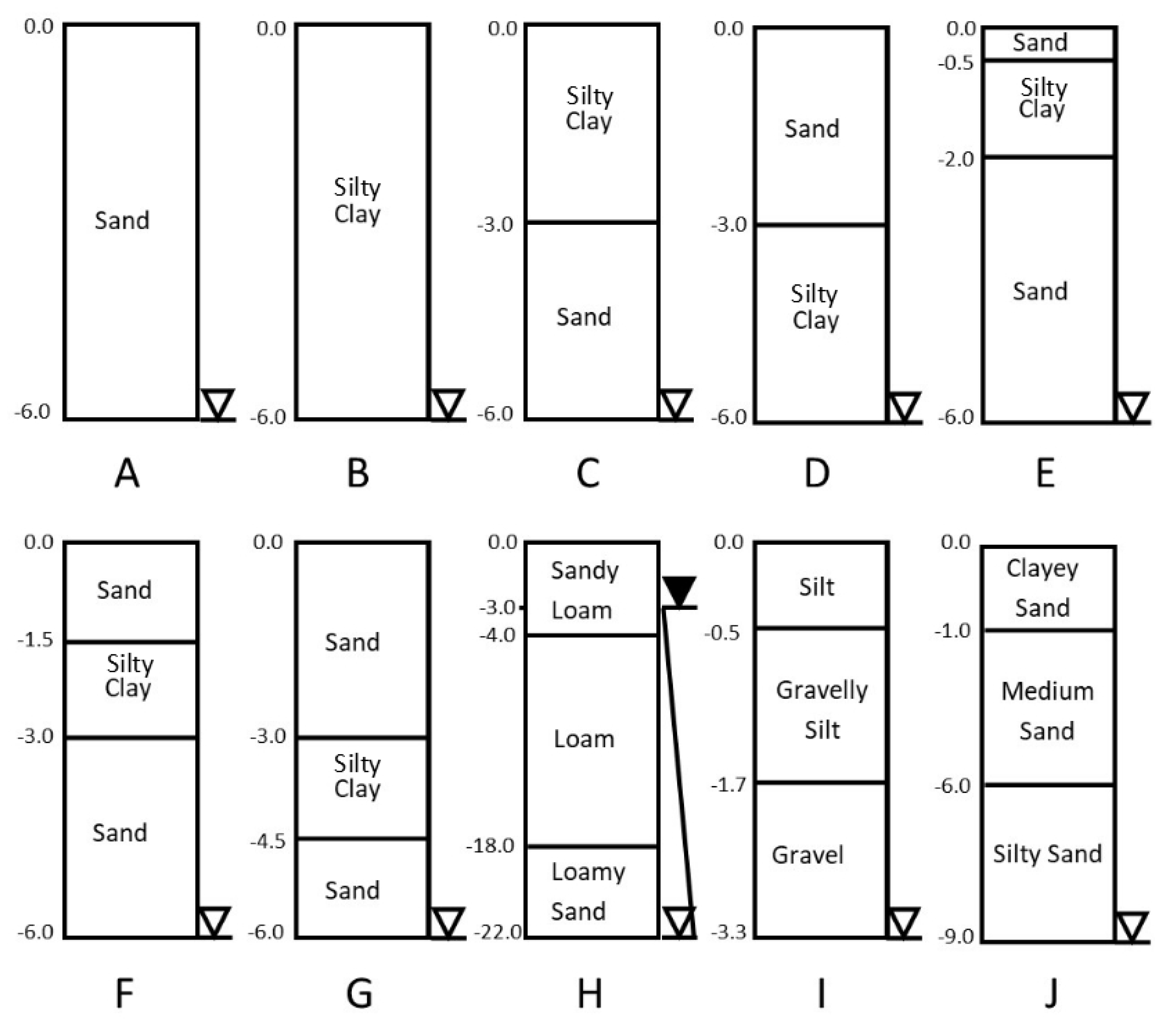
Calculations were performed for 10 soil profiles, as shown in Figure 1. In the first group of profiles (Figure 1A–G) the depth to groundwater table was set to 6m. The homogeneous sand and clay profiles (A and B) were considered as baseline cases. Profiles C and D represent simple layered structures with half of the profile occupied by each soil type. Profiles E–G contain a thin clay layer in sand material, positioned at different depths. This kind of structure has been encountered on glacial outwash plain in the region of Tuchola (northern Poland). Profile H can be considered typical for glacial moraine uplands in the region of Puck (northern Poland), where a confined aquifer is overlaid by multiple layers of glacial till deposits. Finally, profiles I and J are taken from [19] (respectively profiles 1 and 6 in the original paper). All soil materials are characterized by the van Genuchte-Mualem hydraulic functions [25]:

$$S_e=\frac{\theta -{\theta }_r}{{\theta }_s-{\theta }_r}={\left[1+{\left(\alpha \left|h\right|\right)}^{n_g}\right]}^{-m_g},\hspace{1em}k=k_s{k}_r=k_s\sqrt{S_e}{\left[1-{\left(1-S_e^{1/m_g}\right)}^{m_g}\right]}^2$$

(3)

where S_e—effective (normalized) water saturation, θ_r—residual water content, θ_s—water content at fully saturated (or field saturated) conditions, α—parameter related to the air entry pressure (depending on the size of pores), n_g, m_g parameters related to the pore size distribution (m_g = 1 − 1/n_g), k_s—hydraulic conductivity at saturation, k_r—relative hydraulic conductivity. Parameters of each soil material are listed in

Table 1. Parameters of the soil materials.

Soil Type	θr (-)	θs (-)	α (m−1)	ng (-)	ks (m s−1)	θfield Range (-)
Sand [25]	0.045	0.430	14.50	2.68	8.25 × 10−5	0.07−0.10
Silty clay [25]	0.07	0.36	0.50	1.09	5.56 × 10−8	0.24−0.38
Sandy loam [25]	0.065	0.41	7.50	1.89	1.22 × 10−5	0.18−0.26
Loam [25]	0.078	0.43	3.60	1.56	2.89 × 10−6	0.24−0.38
Loamy sand [25]	0.057	0.41	12.40	2.28	4.05 × 10−5	0.18−0.26
Silt [19]	0.021	0.43	0.66	1.68	8.00 × 10−8	0.30−0.36
Gravelly silt [19]	0.016	0.41	2.67	1.45	1.00 × 10−6	0.18−0.36
Gravel [19]	0.001	0.28	49.30	2.19	5.00 × 10−2	0.05−0.10
Clayey sand [19]	0.020	0.40	3.48	1.75	5.00 × 10−5	0.18−0.26
Medium sand [19]	0.019	0.36	3.52	3.18	5.00 × 10−3	0.07−0.10
Silty sand [19]	0.018	0.37	3.48	1.75	5.00 × 10−4	0.18−0.26

. Soils in profiles A–H are characterized by average parameters for their textural classes, as reported in Reference [26]. For profiles I and J we used the parameters from the original study [19].

2.3. Initial and Boundary Conditions

Water flow in vadose zone is driven by precipitation and evaporation fluxes and detailed weather data are necessary to carry out transient analysis. For all profiles we used daily data recorded at the weather station of the Gdańsk University of Technology (Poland) in the period 2011–2015. The average annual precipitation was 550 mm/year. For bare soil scenarios the potential evaporation was calculated by the SWAP code using the Penman-Monteith method, based on the provided values of temperatures, wind speed, relative humidity and solar radiation and the bare soil resistance factor. The average annual potential evaporation for bare soil scenarios was 617 mm/year. The atmospheric boundary condition implemented at the soil surface in SWAP and other similar codes, for example, [13] alternates between flux type and pressure type condition, depending on the state of the soil surface. The infiltration flux is limited by the condition that the maximum pressure at the surface cannot exceed the prescribed ponding depth (in our case equal to zero). Similarly, a limit on the evaporation flux is imposed. In our case we used the limiting condition of minimum allowable water pressure corresponding to the relative humidity of the atmosphere.

In scenarios with grass cover, the detailed model for grass growth and root water uptake was used, as provided in SWAP package [14] and the potential evaporation and transpiration, were calculated by the direct application of the Penman-Monteith equation for specific crop (grass) data. The maximum depth of root zone was set to 50 cm and the root density function decreased nonlinearly with depth. The interception was described by the Hoyningen and Braden model [27,28].

At the bottom of all soil profiles except H a constant value of the water pressure head h = 0 was specified, which corresponds to ground water table. In profile H, h = 19 m was assigned as the bottom boundary condition, representing the piezometric level of a confined aquifer.

Each simulation started with a 5-year warm-up period, in order to establish a realistic initial distribution of the water content in soil profile. In the warm-up period no solute was added to the soil and the concentration was kept equal to zero. Then the same set of weather data was used for the simulation of solute transport, with the solute concentration in precipitation water set to 1 mg/cm³.The bottom boundary condition for solute transport was set to zero concentration gradient. Since the transport equation includes dispersion and the solute concentration in soil water increases due to evaporation and transpiration, the concentration at the bottom increased gradually from 0 to values larger than 1 mg/cm³. Here we report the arrival time of concentration equal to 0.01 mg/cm³ and 0.99 mg/cm³, as indicators of the travel time from surface to the aquifer. In weakly permeable soils the 5-year period of weather data was repeated multiple times before the solute breakthrough occurred.

2.4. Numerical Discretization

Transient simulations of water flow and solute transport were performed using the SWAP code (version 4.01, Wageningen University & Research, Wageningen, The Netherlands) [14]. SWAP solves Equation (1) by means of cell-centred finite difference scheme, with first-order implicit time discretization. The solution accuracy depends on the size of grid cells and the method of calculating the average hydraulic conductivity between adjacent cells, for example, [29]. In our case the soil profiles were discretized using 0.5 cm grid cells in the uppermost 5cm of the profile and 1cm grid cells in the remaining part. The average hydraulic conductivity was calculated as the arithmetic mean. Preliminary calculations showed that further refining of the grid does not lead to appreciable changes in the solution—the recharge and evaporation fluxes obtained using grid sizes of 0.25 cm and 0.5 cm differed by less than 1%. The time step varied in the range 10⁻⁷ to 0.2 days and was adjusted automatically by the SWAP algorithm [14].

2.5. Steady-State Methods for Contaminant Travel Time

Results of transient simulations were compared to simplified estimations of contaminant travel time. We considered 4 methods, which showed the best performance in our previous study focused on homogeneous soils [21]. All methods use the same general formula to calculate the advective velocity ν and the corresponding increment of the travel time Δt over a soil compartment of thickness Δz:

$$v\left(z\right)=\frac{R}{\theta \left(z\right)},$$

(4)

$$\Delta t=\frac{\Delta z\theta \left(z\right)}{R}$$

(5)

where R is the recharge rate, which must be known a priori. The total travel time is obtained by summing Δt for all compartments. The methods differ in the way the values of water content θ in each compartment are estimated. Some methods assume that it is constant for each material layer, while other consider a more detailed distribution of θ in the soil profile. All four simplified methods described below were used to calculate the solute travel time using the average values of recharge obtained for each profile from the SWAP simulations of transient flow. They are summarized in

Table 2. Summary of simplified methods for travel time calculation.

Name	Reference	Method to Calculate θ(z)
hydrostatic	[19]	θ variable in each soil layer,θ(z) = θ(h(z)), h(z) corresponds to hydrostatic equilibrium above the groundwater table
steady flow	[19]	θ variable in each soil layer,θ(z) = θ(h(z)), h(z) obtained from the solution of steady flow equation with uniform flux equal to the average groundwater recharge
Charbeneau and Daniel	[17,30]	θ uniform in each soil layer, calculated from Equation (6)
Witczak and Żurek	[31,32]	θ uniform in each soil layer, chosen from a range of typical field values θfield provided in Reference [29,30]

.

The first method applied in this study is referred to as hydrostatic, since the assumption of hydrostatic equilibrium is used to obtain the distribution of the water content above the groundwater table. While the hydraulic equilibrium condition is not consistent with the occurrence of recharge (downward water flux), it can be considered a reasonable approximation in some situations [19].

The second method, called here steady flow, was suggested in Reference [19]. It makes use of the numerical solution to the steady flow equation, with the lower boundary condition corresponding to the groundwater table position and the condition at the surface representing steady water flux equal to the assumed recharge rate. The solution results in a θ(z) profile, which can be used in conjunction with Equation (4) to estimate the travel time. Sousa et al. [19] pointed out to significant differences between the hydrostatic and steady flow method for a number of soil profiles. Obviously, the hydrostatic profile results in lower values of the water content than steady flow profile, leading to larger velocities and shorter time lags for the same recharge rate. However, our earlier study [21] showed that the hydrostatic assumption may not necessarily be less accurate than steady state assumption, if compared to transient flow and transport simulations. This point is further elaborated in the discussion section.

The third method is taken from Charbeneau and Daniel [30] and Charbeneau [17]. In this case the assumption of gravity-dominated flow is invoked, which means that the hydraulic gradient is equal to unity and thus k(θ) = R. If the relationship between k and θ is known, the corresponding value of the water content can be calculated for each material layer. Specifically, Charbeneau and Daniel [30] used Brooks-Corey type conductivity function, which led to the following expression for the travel time in a homogeneous soil layer:

$$\Delta t=\frac{L}{R}\left[{\theta }_r+\left({\theta }_s-{\theta }_r\right){\left(R/k_s\right)}^{\left(3\lambda +2\right)/\lambda }\right],$$

(6)

Following [17] the values of λ were assumed equal to λ = n_g − 1 for each soil in Table 1. In profile H, which is mostly in the saturated zone, Equation (6) was used only for the upper 3 m of the profile, while in the remaining part Equation (5) was used with θ(z) set to the saturated water content θ_s for each soil layer.

Finally, we also consider the approach proposed by Witczak and Żurek [31] and later modified by Duda et al. [32]. They suggested to use Equations (4) and (5), and provided a range of θ values for different soil types occurring in Poland in typical field conditions. In Table 1 we provide the range of values for each soil, based on the recommendations in Reference [31,32], denoted as θ_field. As a result, for each profile we obtained the lower and upper estimations of the travel time, corresponding to the choice of minimum and maximum values of the water content for the soil materials. In contrast to the previous methods, this one does not require the knowledge of the retention or conductivity functions but its accuracy depend on the choice of θ_field.

3. Results

Table 3. Recharge rates and travel times obtained from numerical simulations of transient flow for non-vegetated soil.

Quantity	Mean Annual Recharge (mm/year)	Recharge/Precipitation Ratio (-)	Arrival Time c = 0.01 mg/cm3 (days)	Arrival Time c = 0.99 mg/cm3 (days)
Profile A	312	0.57	424	661
Profile B	62	0.11	7962	10010
Profile C	61	0.11	4460	6198
Profile D	325	0.59	895	1535
Profile E	316	0.57	746	1030
Profile F	319	0.58	736	1022
Profile G	320	0.58	738	1020
Profile H	247	0.45	10512	12642
Profile I	98	0.18	808	1524
Profile J	195	0.35	794	1308

shows the average annual values of recharge, recharge-precipitation ratio (R/P) and solute arrival time for the case of bare soil. Results for profiles A to G show that the type of soil in the uppermost layer has the largest influence on the value of recharge. Profiles D–G, where the top layer consists of sand, have very similar recharge rates, close to the value calculated for homogeneous sand profile A. The R/P ratio for profiles A and D to G is between 0.5 and 0.6, which is in agreement with previous studies based on numerical modelling [2,21] and can be considered as the upper limit of groundwater recharge under specific climate conditions. It is larger than the maximum values reported in Reference [32] for highly permeable soils (0.36). Smaller R/P ratios were obtained for profiles H (0.45) and J (0.35), where the top layer consists of sandy loam or clayey sand, respectively. In profiles B-C and I the presence of weakly permeable clay or silt at the surface reduced the R/P ratio to 0.11 and 0.18 respectively. We also note that the estimated value of recharge for profiles I and J are considerably smaller than those reported by Sousa et al. [19], based on tracer experiments (469 mm/year and 412 mm/year, respectively), however, this can be probably explained by higher precipitation at the location of the study [19].

In contrast to the value of recharge, the solute travel time seems to be significantly affected by the presence of clay layers embedded deeper in sand (profiles D–G). The travel time in profile D, with the lower half composed of clay is more than twice as long as in homogeneous sand (A). In profiles E–G, where the clay layer is 1.5 m thick, the travel times do not depend on the position of the clay layer within the profiles. All three values are very similar to each other and are between the results for profile A (no clay layer) and profile D (3.0 m clay layer). Due to dispersion, there are visible differences in the arrival times of 1% and 99% of the boundary concentration. The largest relative difference is observed for profile I and the smallest for profile H.

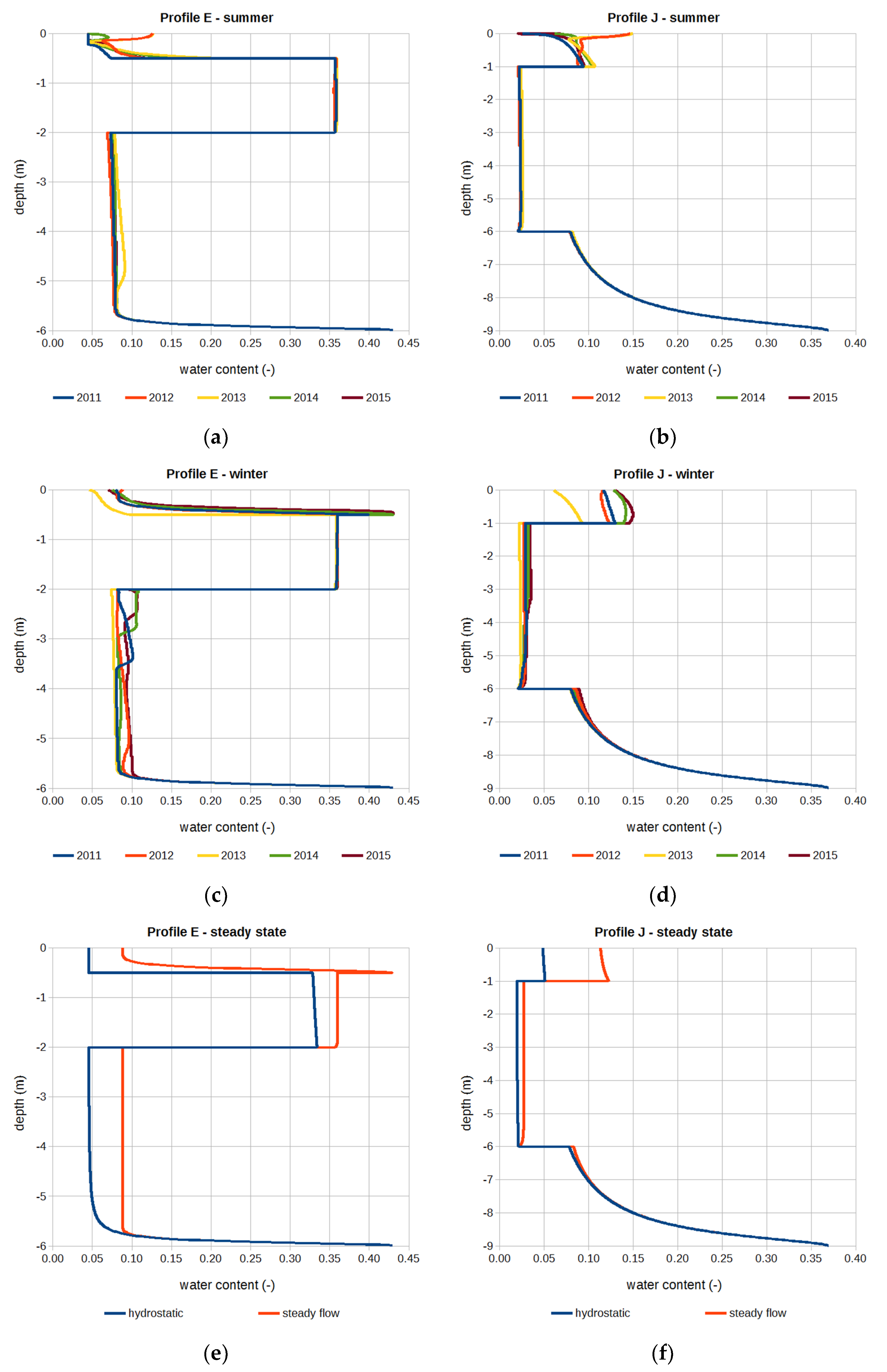
The obtained range of values for the arrival time can be compared with travel time estimates based on steady state approaches, given in

Table 4. Estimates of travel time (days)obtained with steady-state methods for non-vegetated soil.

Method	Hydrostatic	Steady Flow	Charbeneau & Daniel [28]	Witczak & Żurek [29]
Profile A	383	655	629	491–702
Profile B	12,011	12,650	11,445	8477–11,303
Profile C	7106	7948	7164	5565–7539
Profile D	1325	1545	1453	1044–1415
Profile E	849	1124	1030	758–1044
Profile F	879	1155	1057	780–1074
Profile G	880	1141	1045	770–1163
Profile H	12,512	12,747	12,590	12,728–13,078
Profile I	1334	2121	1419	1661–2875
Profile J	1111	1310	830	2003–2883

. For soil profiles with significant proportion of highly permeable materials (A, E–G) the assumption of hydrostatic distribution leads to considerably shorter travel time than the assumption of steady downward flow. These two estimations provide a range of values that is comparable to the range of travel times calculated from transient simulations. As can be seen in Figure 1, for profile E the hydrostatic distribution of θ approximately corresponds to the summer season and the steady flow distribution—to the winter season, with some water ponding on the top of the clay layer. A very similar range of values is obtained using the approach by Witczak and Żurek, with average values of θ_ield reported in Table 1. Considering application of this method to profile E, one has to note that the values of field water content θ_field in Table 1 are in good agreement with the results shown in Figure 1 for the lower part of the profile. However, in the upper sand layer the values are generally larger, especially in winter and the clay layer remain almost fully saturated, with θ = 0.36 corresponding to the upper limit of θ_field in Table 1. The lower estimates from Witczak and Żurek, which are in agreement with the early arrival of solute at the groundwater table, were obtained for smaller values of θ_field from literature, not consistent with the results of simulations.

In profiles B, C and D the discrepancies between estimations based on transient and steady state methods are larger. First, we note that hydrostatic, steady flow and Charbeneau and Daniel methods lead to similar estimates of the travel time and all three are overestimating the solute arrival time, compared to the transient simulations. Also, the results from Witczak and Żurek approach differed from the transient simulations more significantly than in the previous case, for the range of considered water contents. However, the estimate obtained for lower values of the field water content was closer to the breakthrough time obtained from SWAP.

For profile H, all methods based on steady state solutions were close to each other and predicted travel time values close to the arrival time of 99% of input concentration in transient simulation. A good agreement between all methods for this profile can be explained by the fact, that most of its depth is in saturated conditions, with uniquely defined water content value.

In contrast, for profiles I and J the differences between various methods were significant. In profile I the steady flow method overestimated the travel time, while both hydrostatic and Charbeneau and Daniel methods gave results comparable to the values obtained from transient simulations. In profile J all three methods were consistent with transient simulations. In our case the differences between the hydrostatic and steady flow approach were much smaller than reported in Reference [19] for the same profiles but larger recharge values. For profiles I and J the method of Witczak and Żurek appeared to be less accurate than the other simplified methods, substantially overestimating the travel time. This can be explained by very low water content occurring in coarse soil materials (gravel and medium sand), which according to transient flow, steady flow and hydrostatic results (Figure 2) is below the lower limit of field water content given in Table 1. Thus, the resulting advective velocity is larger than predicted by the method of Witczak and Żurek.

In

Table 5. Recharge rates and travel times obtained from numerical simulations of transient flow for soil with grass cover.

Quantity	Mean Annual Recharge (mm/year)	Recharge/Precipitation Ratio (-)	Arrival Time c = 0.01 mg/cm3 (days)	Arrival Time c = 0.99 mg/cm3 (days)
Profile A	220	0.40	531	806
Profile B	38	0.07	11,782	13,555
Profile C	38	0.07	6336	8706
Profile D	223	0.42	1480	1876
Profile E	215	0.39	851	1526
Profile F	224	0.41	834	1503
Profile G	224	0.41	830	1501
Profile H	195	0.35	12,956	15,477
Profile I	52	0.09	963	1852
Profile J	156	0.28	1314	1660

we report recharge and travel time values obtained with transient simulations for soil with grass cover. There is a significant reduction of recharge, ranging from 22% for profile H to 50% for profile I. In our previous study [21], we observed even larger decrease in homogeneous profiles of sand and silty clay. However, in that work, we assumed that the reference evapotranspiration corresponds entirely to transpiration and the root density decreases linearly with depth. Here, a more detailed description is used, where only a part of the reference evapotranspiration is assigned to transpiration depending on the growth of plants and the root density distribution is such that great majority of roots is very close to the soil surface. Consequently, there is less difference between the bare soil and grass scenarios. Keese at al. [2] also reported more significant reduction of recharge due to vegetation than obtained here, however their studies focused on locations with much higher potential evapotranspiration. The influence of various models of root water uptake and their parameters should be further investigated in conjunction with soil textural variability and climate.

The travel time estimates obtained with steady state approximations for vegetated soils are summarized in

Table 6. Estimates of travel time (days) obtained with steady-state methods for soil with grass cover.

Method	Hydrostatic	Steady Flow	Charbeneau & Daniel [28]	Witczak & Żurek [29]
Profile A	543	892	857	697–995
Profile B	19,598	20,550	18,392	13,832–21,900
Profile C	11,407	12,630	11,271	8933–13,832
Profile D	1880	2170	2027	1482–2295
Profile E	1283	1661	1514	1146–1732
Profile F	1241	1598	1457	1100–1662
Profile G	1257	1598	1457	1100–1662
Profile H	15,849	16,120	15,926	16,116–16,565
Profile I	2513	3905	2454	3131–5419
Profile J	1388	1623	1011	2504–3603

. Again, the performance of simplified methods is case-dependent. In particular, for profiles E–G the hydrostatic and steady flow methods cannot capture the early breakthrough time of the solute and for profiles B–D they considerably overestimate the travel time even for c = 0.99 mg/cm³. In contrast, both methods still perform well in the case of homogeneous sand. For profiles B–D the method of Witczak and Żurek provides a range of time lag values more comparable to the transient simulations but again, this is due to the use of smaller, literature-based water content, not corresponding to the simulation results. In profile I all steady state approximations significantly overpredict the solute travel time. On the other hand, in profile J the hydrostatic and steady flow methods produce results close to the transient flow simulations, while the method of Charbeneau and Daniel leads to shorter arrival time than the one obtained from transient flow simulations. Similarly to the non-vegetated case, the method of Witczak and Żurek predicts much longer travel times than SWAP calculations.

4. Summary and Conclusions

Numerical simulations of transient flow and transport in layered soil profiles were compared to simplified methods of estimating solute travel time, based on the assumption of steady flow and purely advective transport. Even with the relatively small value of dispersion constant used in this study (6 cm), the arrival of the solute at ground water table was spread in time. Thus, the unsaturated zone time lag should be considered as a time interval, rather than a single value. The simplified methods reproduced the results of transient simulations with mixed success. They performed best for profiles dominated by sand materials without vegetation. In the case of vegetated profiles or profiles with fine-textured material at the surface, the simplified method were generally not able to capture the earlier arrival time of concentration c = 0.01 mg/cm³, the results were closer to the travel time for c = 0.99 mg/cm³ but in some cases the time was greatly overestimated. It is difficult to distinguish any of the simple methods as superior to the other ones. The methods based on hydrostatic and steady-state distribution of the water content can be viewed as complementary in the case of coarse-textured soils but for fine textured soils they both predict time lags significantly longer than the transient simulations. The method based on the use of average values of the water content [29] performed quite well despite its simplicity but the agreement with transient simulations was often obtained for values of the water content taken from the literature and not corresponding to the particular setting under consideration. Thus, from the point of view of practical application of this method, the use of water content values measured in the field may not necessarily lead to improved results.

This study confirmed the utility of numerical modelling as a tool to estimate groundwater recharge, especially due to the ease of implementing different scenarios related to lithology, vegetation and weather data. The obtained results are in agreement with earlier reports, showing the importance of climate, soil texture in the surface layer and vegetation as the main controls of groundwater recharge [2,3,4,5].

References

- Scanlon, B.R.; Christman, M.; Reedy, R.C.; Porro, I.; Simunek, J.; Flerchinger, G.N. Intercode comparisons for simulating water balance of surficial sediments in semiarid regions. Water Resour. Res. 2002, 38. [Google Scholar] [CrossRef]
- Keese, K.E.; Scanlon, B.R.; Reedy, R.C. Assessing controls on diffuse groundwater recharge using unsaturated flow modeling. Water Resour. Res. 2005, 41. [Google Scholar] [CrossRef] [Green Version]
- Ordens, C.M.; Post, V.E.; Werner, A.D.; Hutson, J.L. Influence of model conceptualisation on one-dimensional recharge quantification: Uley South, South Australia. Hydrogeol. J. 2014, 22, 795–805. [Google Scholar] [CrossRef]
- Vero, S.E.; Ibrahim, T.G.; Creamer, R.E.; Grant, J.; Healy, M.G.; Henry, T.; Kramers, G.; Richards, K.G.; Fenton, O. Consequences of varied soil hydraulic and meteorological complexity on unsaturated zone time lag estimates. J. Contam. Hydrol. 2014, 170, 53–67. [Google Scholar] [CrossRef] [PubMed] [Green Version]
- Wang, T.; Franz, T.E.; Zlotnik, V.A. Controls of soil hydraulic characteristics on modeling groundwater recharge under different climatic conditions. J. Hydrol. 2015, 521, 470–481. [Google Scholar] [CrossRef]
- Fenton, O.; Vero, S.; Ibrahim, T.G.; Murphy, P.N.C.; Sherriff, S.C.; Ó hUallacháin, D. Consequences of using different soil texture determination methodologies for soil physical quality and unsaturated zone time lag estimates. J. Contam. Hydrol. 2015, 182, 16–24. [Google Scholar] [CrossRef] [PubMed]
- Vero, S.E.; Healy, M.G.; Henry, T.; Creamer, R.E.; Ibrahim, T.G.; Richards, K.G.; Mellander, P.-E.; McDonald, N.T.; Fenton, O. A framework for determining unsaturated zone water quality time lags at catchment scale. Agric. Ecosyst. Environ. 2017, 236, 234–242. [Google Scholar] [CrossRef]
- Batalha, M.S.; Barbosa, M.C.; Faybishenko, B.; van Genuchten, M.T. Effect of temporal averaging of meteorological data on predictions of groundwater recharge. J. Hydrol. Hydromech. 2018, 66, 143–152. [Google Scholar] [CrossRef] [Green Version]
- Szymkiewicz, A.; Gumuła-Kawęcka, A.; Šimůnek, J.; Leterme, B.; Beegum, S.; Jaworska-Szulc, B.; Pruszkowska-Cacers, M.; Gorczewska-Langner, W.; Jacques, D. Simulations of freshwater lens recharge and salt/freshwater interfaces using the HYDRUS and SWI2 packages for MODFLOW. J. Hydrol. Hydromech. 2018, 66, 246–256. [Google Scholar] [CrossRef] [Green Version]
- Bashir, R.; Pastora Chevez, E. Spatial and seasonal variations of water and salt movement in the vadose zone at salt-impacted sites. Water 2018, 10, 1833. [Google Scholar] [CrossRef]
- Zhou, Y.; Wang, X.S.; Han, P.F. Depth-dependent seasonal variation of soil water in a thick vadose zone in the Badain Jaran Desert, China. Water 2018, 10, 1719. [Google Scholar] [CrossRef]
- Beegum, S.; Šimůnek, J.; Szymkiewicz, A.; Sudheer, K.P.; Nambi, I.M. Implementation of solute transport in the vadose zone into the ‘HYDRUS package for MODFLOW’. Groundwater 2018. [Google Scholar] [CrossRef]
- Šimůnek, J.; Šejna, M.; Saito, H.; Sakai, M.; van Genuchten, M.T. The HYDRUS-1D Software Package for Simulating the One-Dimensional Movement of Water, Heat, and Multiple Solutes in Variably-Saturated Media, Version 4.0; HYDRUS Software Series 3; University of California: Riverside, CA, USA, 2008. [Google Scholar]
- Kroes, J.G.; van Dam, J.C.; Bartholomeus, R.P.; Groenendijk, P.; Heinen, M.; Hendriks, R.F.A.; Mulder, H.M.; Supit, I.; van Walsum, P.E.V. SWAP Version 4. Theory Description and User Manual; Report 2780; Wageningen University & Research: Wageningen, The Netherlands, 2017. [Google Scholar]
- Fayer, M.J.; Jones, T.L. UNSAT-H Version 2.0: Unsaturated Soil Water and Heat Flow Model (No. PNL-6779); Pacific Northwest Lab.: Richland, WA, USA, 1990.
- Schroeder, P.R.; Dozier, T.S.; Zappi, P.A.; McEnroe, B.M.; Sjostrom, J.W.; Peton, R.L. The Hydrologic Evaluation of Landfill Performance (HELP) Model: Engineering Documentation for Version 3; EPA/600/R-94/168b; US. Environmental Protection Agency, Risk Reduction Engineering Laboratory: Cincinnati, OH, USA, 1994.
- Charbeneau, R.J. Groundwater Hydraulics and Pollutant Transport; Waveland Press: Long Grove, IL, USA, 2006; ISBN 1478608315. [Google Scholar]
- Fenton, O.; Schulte, R.P.; Jordan, P.; Lalor, S.T.; Richards, K.G. Time lag: A methodology for the estimation of vertical and horizontal travel and flushing timescales to nitrate threshold concentrations in Irish aquifers. Environ. Sci. Policy 2011, 14, 419–431. [Google Scholar] [CrossRef]
- Sousa, M.R.; Jones, J.P.; Frind, E.O.; Rudolph, D.L. A simple method to assess unsaturated zone time lag in the travel time from ground surface to receptor. J. Contam. Hydrol. 2013, 144, 138–151. [Google Scholar] [CrossRef]
- Potrykus, D.; Gumuła-Kawęcka, A.; Jaworska-Szulc, B.; Pruszkowska-Caceres, M.; Szymkiewicz, A. Assessing groundwater vulnerability to pollution in the Puck region (denudation moraine upland) using vertical seepage method. E3S Web Conf. 2018, 44, 00147. [Google Scholar] [CrossRef]
- Szymkiewicz, A.; Gumuła-Kawęcka, A.; Potrykus, D.; Jaworska-Szulc, B.; Pruszkowska-Caceres, M.; Gorczewska-Langner, W. Estimation of conservative contaminant travel time through vadose zone based on transient and steady flow approaches. Water 2018, 10, 1417. [Google Scholar] [CrossRef]
- Feddes, R.A.; Kowalik, P.J.; Zaradny, H. Simulation of Field Water Use and Crop Yield; Simulation Monographs; Pudoc: Wageningen, The Netherlands, 1978. [Google Scholar]
- Šimůnek, J.; van Genuchten, M.T. Modeling nonequilibrium flow and transport processes using HYDRUS. Vadose Zone J. 2008, 7, 782–797. [Google Scholar] [CrossRef]
- Szymkiewicz, A.; Lewandowska, J. Unified macroscopic model for unsaturated water flow in soils of bimodal porosity. Hydrol. Sci. J. 2006, 51, 1106–1124. [Google Scholar] [CrossRef] [Green Version]
- Van Genuchten, M.T. A closed-form equation for predicting the hydraulic conductivity of unsaturated soils. Soil Sci. Soc. Am. J. 1980, 44, 892–898. [Google Scholar] [CrossRef]
- Carsel, R.F.; Parrish, R.S. Developing joint probability distributions of soil water retention characteristics. Water Resour. Res. 1988, 24, 755–769. [Google Scholar] [CrossRef]
- Von Hoyningen-Hüne, J. Die Interception des Niederschlags in landwirtschaftlichen Beständen. Schr. DVWK 1983, 57, 1–53. [Google Scholar]
- Braden, H. Ein Energiehaushalts- und Verdunstungsmodell für Wasser und Stoffhaushaltuntersuchungen landwirtschaftlich genutzer Einzugsgebiete. Mitt. Deutsch.Bodenkd. Geselschaft 1985, 42, 294–299. (In German) [Google Scholar]
- Szymkiewicz, A. Approximation of internodal conductivities in numerical simulation of one-dimensional infiltration, drainage, and capillary rise in unsaturated soils. Water Resour. Res. 2009, 45, W10403. [Google Scholar] [CrossRef]
- Charbeneau, R.J.; Daniel, D.E. Contaminant transport in unsaturated flow. In Handbook of Hydrology; Maidment, D.R., Ed.; McGraw-Hill: New York, NY, USA, 1993. [Google Scholar]
- Witczak, S.; Żurek, A. Wykorzystanie map glebowo-rolniczych w ocenie ochronnej roli gleb dla wód podziemnych (Use of soil-agricultural maps in the evolution of protective role of soil for groundwater). In Metodyczne Podstawy Ochrony Wód Podziemnych; Methodical Principles of Groundwater Protection; Kleczkowski, A., Ed.; AkademiaGórniczo-Hutnicza: Kraków, Poland, 1994. (In Polish) [Google Scholar]
- Duda, R.; Winid, B.; Zdechlik, R.; Stępień, M. Metodyka Wyboru Optymalnej Metody Wyznaczania Zasięgu Stref Ochronnych Ujęć Zwykłych Wód Podziemnych z Uwzględnieniem Warunków Hydrogeologicznych Obszaru RZGW w Krakowie; Methodology of Selecting the Optimal Method of the Wellhead Protection Area Delineation Taking into Account the Hydrogeological Conditions in Areas Administered by the Regional Water Management Board in Cracow; Akademia Górniczo-Hutnicza: Kraków, Poland, 2013; ISBN 9788388927294. (In Polish) [Google Scholar]
Figure 1.
Soil profiles used in numerical simulations.
Figure 2.
Volumetric water content distributions obtained from transient simulations and steady state approximations for soil profiles E and J, non-vegetated soil, (a) profile E, summer (30 Jun.), (b) profile J, summer; (c) profile E, winter (31 Dec.); (d) profile J, winter; (e) profile E, steady state, (f) profile J, steady state.