Moisture Distribution in Sloping Black Soil Farmland during the Freeze–Thaw Period in Northeastern China

1
The Institution of Water and Environment Research, Dalian University of Technology, Dalian 116024, China
2
Institute of Soil and Water Conservation, Heilongjiang Province Hydraulic Research Institute, Harbin 150080, China
3
Institute of Water Resources for Pastoral Area, Huhhot 010021, China
*
Author to whom correspondence should be addressed.
Water 2019, 11(3), 536; https://doi.org/10.3390/w11030536
Submission received: 30 January 2019
/
Revised: 27 February 2019
/
Accepted: 6 March 2019
/
Published: 14 March 2019
(This article belongs to the Special Issue Application of the China Meteorological Assimilation Driving Datasets for the SWAT Model (CMADS) in East Asia)
Abstract
:This paper outlines dynamics of near-surface hydrothermal processes and analyzes the characteristics of moisture distribution during the freeze–thaw period in a typical black soil zone around Harbin, Northeastern China, a region with a moderate depth of seasonally frozen ground and one of the most important granaries in China. At Field Site 1, we analyzed the soil temperature and soil moisture content data from November 2011 to April 2012 from soil depths of 1, 5, 10, and 15 cm in sunny slope, and from depths of 1, 5, and 10 cm in shady slope black soil farmland. At Field Site 2, soil samples were collected from a 168 m long sloping black soil field at locations 10, 50, 100, and 150 m from the bottom of the slope at different depths of 0–1 cm, 1–5 cm, and 5–10 cm at the same location. Analysis of the monitored Site 1 soil temperature and soil moisture content data showed that the soil moisture content and soil temperature fit line is consistent with a Gaussian distribution rather than a linear distribution during the freeze–thaw period. The soil moisture content and time with temperature fit line is in accordance with a Gaussian distribution during the freeze–thaw period. Site 2 soil samples were analyzed, and the soil moisture contents of the sloping black soil farmland were obtained during six different freeze–thaw periods. It was verified that the soil moisture content and time with temperature fit line is in accordance with a Gaussian distribution during the six different freeze–thaw periods. The maximum surface soil moisture content was reached during the early freeze–thaw period, which is consistent with the natural phenomenon of early spring peak soil moisture content under temperature rise and snow melt. The soil moisture contents gradually increased from the top to the bottom in sloping black soil farmland during the freeze–thaw period. Since the soil moisture content is related to soil temperature during the freeze–thaw cycle, we validated the correlation between soil temperature spatiotemporal China Meteorological Assimilation Driving Datasets for the Soil and Water Assessment Tool (SWAT) model–Soil Temperature (CMADS-ST) data and monitored data. The practicality of CMADS-ST in black soil slope farmland in the seasonal frozen ground zone of the study area is very good. This research has important significance for decision-making for protecting water and soil environments in black soil slope farmland.
1. Introduction
In this paper, the distribution of soil moisture in sloping black soil farmland during freeze–thaw cycles in Northeastern China is discussed. Soil moisture has great impacts on food security, human health, and ecosystem function; however, it is difficult to quantify the regional distribution and dynamics of soil moisture [1]. There are many factors that can influence soil moisture distribution. Previous research has shown that the soil moisture content and freezing/thawing processes have strong correlations with soil temperature [2]. Research in the Loess Plateau of China indicated that soil clay content and topography were the most important factors affecting soil water content at soil depths of 0–500 cm in the gully [3,4]. Studies in Northwestern China showed that land use and vegetation also have impacts on the soil moisture distribution [5,6,7,8]. Besides physicochemical factors, rainfall-runoff processes could also have great impacts on the soil moisture dynamics [9]. Furthermore, the antecedent soil moisture conditions also play an important role in rainfall-triggered shallow landslide events, which has been debated by Lazzari et al [10]. Large seasonal frozen soil regions exist all over the world. The freeze–thaw period is an important process influencing the soil moisture dynamic process. Snowmelt runoff is an important part of spring runoff and has an important impact on soil moisture distribution in frozen soil regions [11,12]. Studies of the soil moisture contents during freeze–thaw periods have been conducted. For instance, researchers have quantitatively studied the heat transfer of soil moisture during the freezing period and have provided water–heat coupling equations for freezing soil [13,14,15,16]. The first such equation was the moisture migration model, published in 1973 [17], which is based on the theory that the migration of unfrozen water in partially frozen ground is similar to the migration of moisture in unsaturated soil. Quantitative studies have produced numerical solutions for modeling water-heat coupling in freeze–thawing soils [18]. The application of these models to soils at mid and high latitudes requires the inclusion of freeze–thaw processes within the soil and the accumulation and ablation of snow cover [19]. Simulated soil temperature and soil liquid water contents are comparable to measured values, which show the isolating effect of snow cover. Under freeze–thaw conditions, plots have been studied to determine the effects of soil moisture on freeze–thaw processes [20,21,22,23,24]. The processes of soil freeze–thawing and the dynamic variations of moisture–heat transfer, including the soil water content, temperature, frost depth, soil evaporation, and water flux in the seasonal freeze–thawing period, were used in a one-dimensional simulation of soil water and heat dynamics during the winter period [25]. The importance of the heterogeneity of the infiltration process that results from the effects of the ground freezing, snow melting (including the contact between the melting snow cover and the soil), and unsaturated flow, is emphasized [26].
The black soil zone in Northeastern China is located in a region with a moderate depth of seasonally frozen ground (−2 ± 1 m), and which is one of the most important granaries in China. Plain-and-hill sloping black soil farmland (<10°) accounts for 60% of the total cultivated land (9.5 × 10⁶ ha in Heilongjiang Province) in the black soil zone [27,28,29,30]. However, few studies have been conducted to determine the distribution of soil moisture with depth over time in sloping black soil farmland in Northeastern China during freeze–thaw cycles. Under the relevant boundary conditions of sloping farmlands in black soil plains and hills, exploring the changing process of freeze–thawing soils with soil moisture, and correlations between soil moisture and temperature, is important for protecting soil moisture in sloping black soil farmland. Besides this, soil temperature plays a key role in the land surface processes, since this parameter affects a series of physical, chemical, and biological processes in the soil, such as water and heat fluxes [31]. In the study of moisture distribution during the freeze–thaw period, it is very important to obtain soil temperature changes during soil freezing and thawing. However, soil temperature datasets are often difficult to obtain, requiring a large amount of equipment and time. Some researchers have used reanalysis datasets to investigate the relationship between soil temperature and soil moisture and obtained satisfactory results [32,33,34,35,36]. The China meteorological assimilation driving datasets for the soil and water assessment tool (SWAT) model–soil temperature (CMADS-ST) are the soil temperature reanalysis datasets of CMADS series datasets developed by Prof. Dr. Xianyong Meng from China and have attracted great attention [37]. CMADS incorporated technologies of local analysis and prediction system/space time multiscale analysis system (LAPS/STMAS) and was constructed using multiple technologies and scientific methods, including loop nesting of data, the projection of resampling models, and bilinear interpolation. The CMADS has been used successfully in different basins, such as the Heihe River Basin, Juntanghu Basin, Manas River Basin, and Han River Basin, indicating good applicability of CMADS in East Asia [38,39,40,41,42,43,44,45,46,47,48,49,50]. However, the relative studies mainly focused on the surface hydrological process and meteorological data, whereas the application of the CMADS-ST to soil temperature and soil moisture distribution has been rarely studied, especially in the black soil zone [51,52,53,54].
In this background, it is necessary to compare and verify the applicability of the reanalysis datasets of CMADS-ST. Therefore, the aims of this paper are:
- (1)
- To analyze the relationship between the reanalysis datasets of CMADS-ST and the observed values;
- (2)
- to study the characteristics of moisture distribution during the freeze–thaw period; and
- (3)
- to identify the effects of soil temperature on the moisture distribution in the black soil zone.
2. Materials and Methods
2.1. Experimental Site
Site 1: The Water Conservancy Comprehensive Experimental Research Center of Heilongjiang Province, China, is located on the outskirts of Harbin. Here, a typical moderately deep seasonally frozen ground experimental observation field was established from November 2011 to April 2012. Site 1 for field observations of natural freezing and thawing is located at 45°38′16.48″ N 126°22′51.31″ W at an elevation of 138 m a.s.l. and has a 5° slope. The site contains sunny slope and shady slope black soil farmland. The lowest monthly average temperature occurs in January, which was −24.6 °C in 2012 and −21.3 °C in 2014.
Site 2: An area of sloping black soil farmland in Longquan Town, Bayan County, Heilongjiang Province, China, was chosen as the experimental observation area, as shown in Figure 1. Site 2 for field observations of natural freezing and thawing is located at 46°12′08″ N 127°28′34″ W at an elevation of 158 m a.s.l. and has a 1.3° slope with a length of 168 m.
The climate of the research zone is continental monsoon and cold temperate. The multi-year mean annual air temperature is 5.6 °C, the lowest monthly average temperature is −15.8 °C, and the mean annual precipitation is 423 mm. In the region of seasonally frozen ground, precipitation mainly occurs from May to September each year, with less precipitation occurring during late autumn, winter, and early spring. Four meteorological seasons occur during the year: spring, summer, autumn, and winter. The summer season is hot and rainy, and the winter season is cold and long. Planting occurs during the spring season in the middle of May, and crops are harvested during the autumn in early October. Crops are planted each year in monoculture using ridge tillage, and the main crop grown in the region is corn. The area consists of sloping black soil farmlands in the region of moderately deep seasonal frozen ground of Northeastern China. The average depth of the seasonal frozen ground between the years 1949 and 2010 was 1.95 ± 0.25 m at the site.
2.2. Experiment and Data Collection
Site 1: After the autumn harvest in 2011, soil temperature and moisture sensors were buried at depths of 1, 5, 10, and 15 cm in sunny slope black soil farmland, and at depths of 1, 5, and 10 cm in shady slope black soil farmland during the freeze–thaw periods. After the autumn harvest in 2013, the level was used to measure the height, the distance of the measuring tape is the slope distance, and then the slope of the slope farmland was calculated. Site 2: The soil temperature and moisture sensors were buried at depths of 1, 5, 10, and 15 cm in slope black soil farmland at a distance of 100 m from the bottom of the slope during the freeze–thaw periods. We observed the soil moisture content and temperature at various depths during the freeze–thaw period for the plots containing black soils in the region of seasonally frozen ground at sites 1 and 2. Precautions were taken during the installation of sensors used in the field, especially for the problem of soil temperature and the direction in which the soil moisture sensor was buried. For sites 1 and 2, firstly, pits were dug to a depth of 60 cm and a diameter of about 40 cm in the black soil slope farmland after the autumn harvest. When installing the soil temperature and soil moisture sensors, special attention was paid to the direction of burial. The direction of the sensor probe was toward the top of the slope. The soil temperature and soil moisture sensor were aligned parallel to the slope. The depth of the sloping farmland from the surface of the sloping farmland was measured with a steel tape measure. Finally, the soil from the pit was backfilled into the pit of the embedded instrument, and the compaction was made to be as close as possible to the original surface. The soil moisture and soil temperature sensor probes were oriented in the direction of the top of the slope to prevent disturbance of the excavation and to prevent the soil moisture from collecting, as the disturbance would affect the monitoring of soil moisture content.
Site 1: we collected data on the soil temperature and volumetric soil moisture content from November 2011 to April 2012 at depths of 1, 5, 10, and 15 cm in sunny slope black soil farmland, and at depths of 1, 5, and 10 cm in shady slope black soil farmland.
Site 2: Soil samples were collected from the 168 m long sloping black soil field at locations 10, 50, 100, and 150 m from the bottom of the slope for testing and analysis. During the freeze–thaw periods, including the pre-freezing period, freezing period, early freeze–thaw period, mid freeze–thaw period, late freeze–thaw period, and post-thawing period, surface-soil samples were taken from the sloping black soil farmland at depths of 0–1 cm, 1–5 cm, and 5–10 cm at the same location. The soil samples were tested to obtain mass soil moisture content (different from the volumetric soil moisture content obtained from Site 1), soil ammonia nitrogen content, and soil available phosphorus content. This paper only studies the distribution of soil moisture content; the distribution of soil ammonia nitrogen and soil available phosphorus are studied separately. At Site 2, soil layering temperature data were collected at hourly intervals on the day of sampling. The soil temperature layering depths were 1, 5, 10, and 15 cm, respectively. Site 2 sampling points, in the pre-freezing period, were at distances of 10, 50, 100, and 150 m from the bottom of the slope, and sampling from the surface of the black soil slope farmland was performed every 5 cm to 50 cm depth. An aluminum box was used to collect the marked soil. The soil samples were weighed and dried in the laboratory to obtain the soil bulk density.
We used high-resolution time series data from the CMADS-ST to conduct spatial- and temporal-scale analyses of meteorological data. We investigated the collection of the CMADS soil temperature and precipitation data with the test monitoring location close to the coordinates of the points, and the time synchronization of data. The moisture in the plow layer of black soils is significantly different at different depths during the freeze–thaw process depending on precipitation and soil temperature.
3. Results
3.1. Observed Soil Moisture and Soil Temperature Values
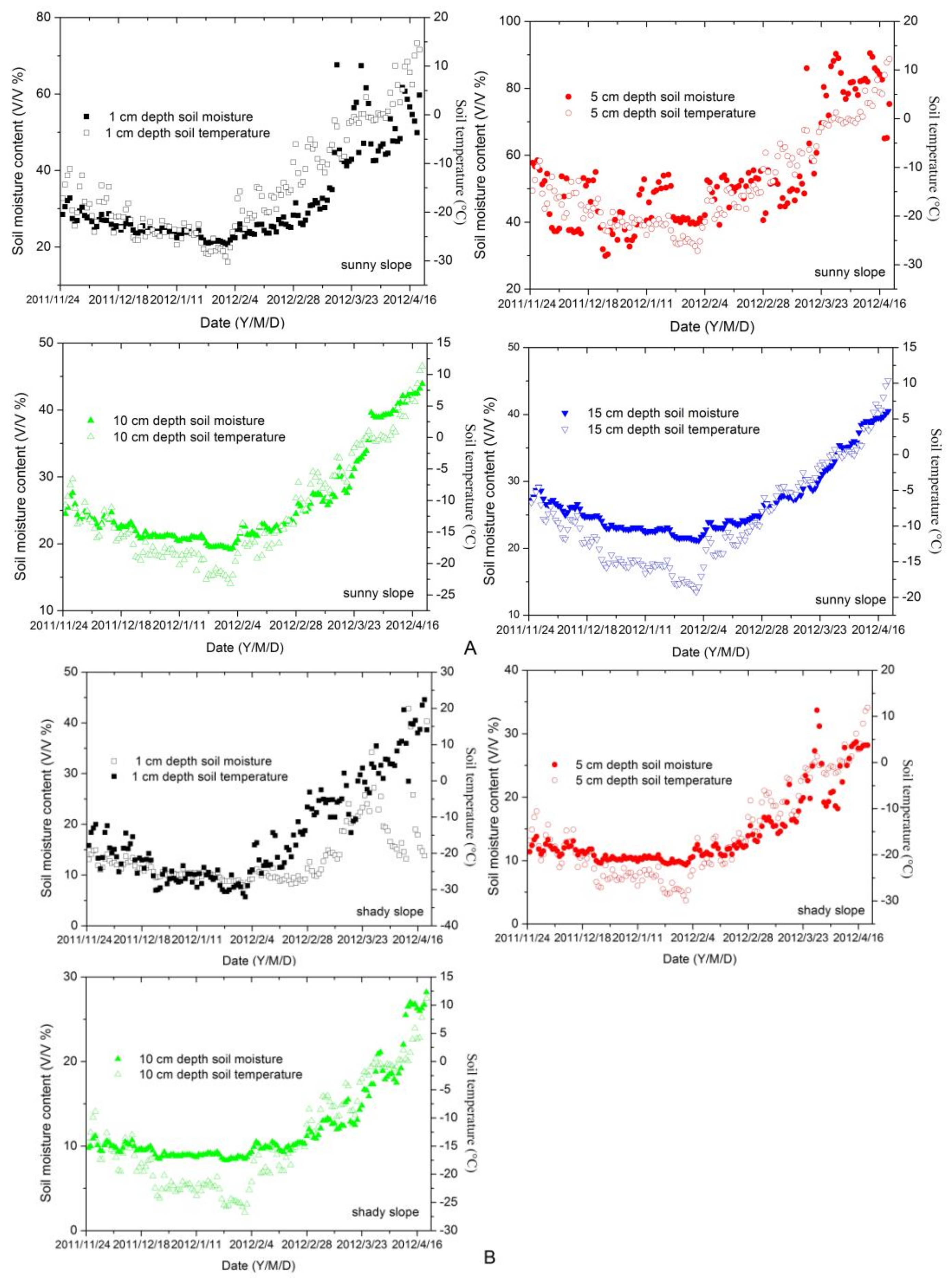
Figure 2 shows the soil moisture contents and soil temperature scatter diagrams that were observed at various depths during the 2011–2012 freeze–thaw period, including at the sunny slope depths of 1, 5, 10, and 15 cm and the shady slope depths of 1, 5, and 10 cm. The observation dates were from 20 November 2011 to18 April 2012. The daily volumetric soil moisture contents and soil temperatures were measured at experimental Site 1.
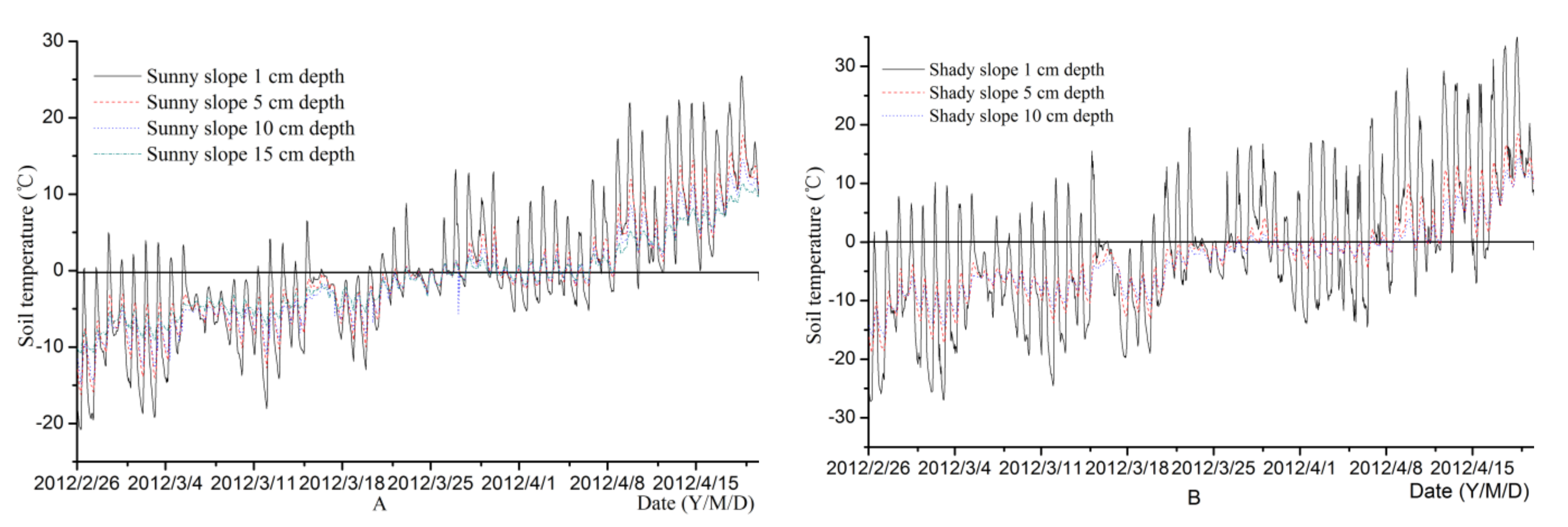
Figure 2A shows that, for the sunny slope, the surface black soil temperature at a depth of 1 cm in the study area ranged from −31.9to 15 °C. The surface of the black soil at a depth of 1 cm was seasonally covered by ice and snow and experienced approximately 39 freeze–thaw cycles in the spring season of 2012. The shady slope experienced 47 freeze–thaw cycles in the spring season of 2012, as shown in Figure 3.
The distribution of soil temperature and soil moisture was measured within the black soil plow layer during the freeze–thaw process. The soil temperature and moisture data were obtained from typical moderately deep seasonally frozen ground. This was an experimental observation field setup shown in Figure 2. Soil temperature changes affect the variations of soil moisture contents in seasonally frozen ground regions with black topsoil during soil freezing and thawing period. This shows that the soils under the plow layer in moderately deep seasonally frozen regions of black soil are usually subjected to a freeze–thaw period of approximately five months.
Figure 2 shows the distribution of the soil moisture contents and soil temperature at depths of 1, 5, 10, and 15 cm in the sunny slope black soil farmland and at depths of 1, 5, and 10 cm in the shady slope black soil farmland during the freeze–thaw period. The abscissa is always the same time of the freeze–thaw period from 20 November 2011 to18 April 2012.The left side of the ordinate Y-axis represents the soil temperature, and the temperature scale range is different at different depths. The right side of the ordinate Y-axis represents the soil moisture content, and the soil moisture content scale range is also different at different depths. Solid black squares, solid red circles, solid green up triangles, and solid blue down triangles represent soil moisture at depths of 1, 5, 10, and 15 cm, respectively. Open symbols represent soil temperature, and different symbol colors represent soil moisture content at different depths of soil temperature. It was found that the scatter patterns of soil moisture content and soil temperature are similar in the same freeze–thaw cycle period, at different depths.
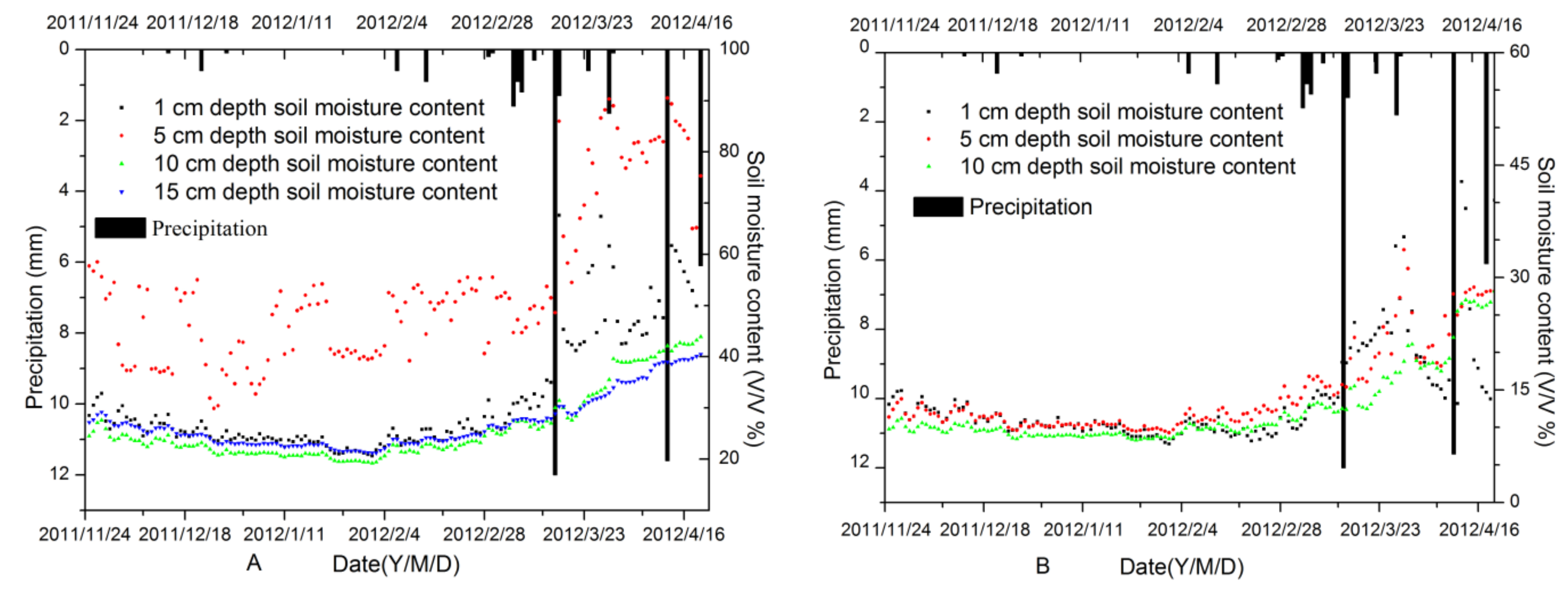
Figure 4 shows changes in the soil moisture contents in the plow layer of black soils with temperature during a period of freeze–thaw cycles in an area of seasonal frozen ground. This figure shows that the moisture in the plow layer of black soils is significantly different at different depths during the freeze–thaw process depending on precipitation and soil temperature.
Figure 4 shows the relationships between precipitation and soil moisture contents at different depths during the freeze–thaw period. Precipitation data were obtained from the CMADS data-sharing website (http://www.cmads.org). The surface temperatures of the black soils at different depths (1, 5, and 10 cm) were measured at the experimental observation Site 1.
During the winter, precipitation occurs in the form of snowfall. The black sagging histogram in Figure 4 shows the precipitation in the study area. During the freeze–thaw period from20 November 2011 to18 April 2012, the daily maximum snowfall was 12 mm snow water equivalent. The total precipitation during the freeze–thaw period accounted for 17.3% of the annual amount (10 April 2011–10 April 2012).
3.2. The Relationship between Soil Moisture and Soil Temperature
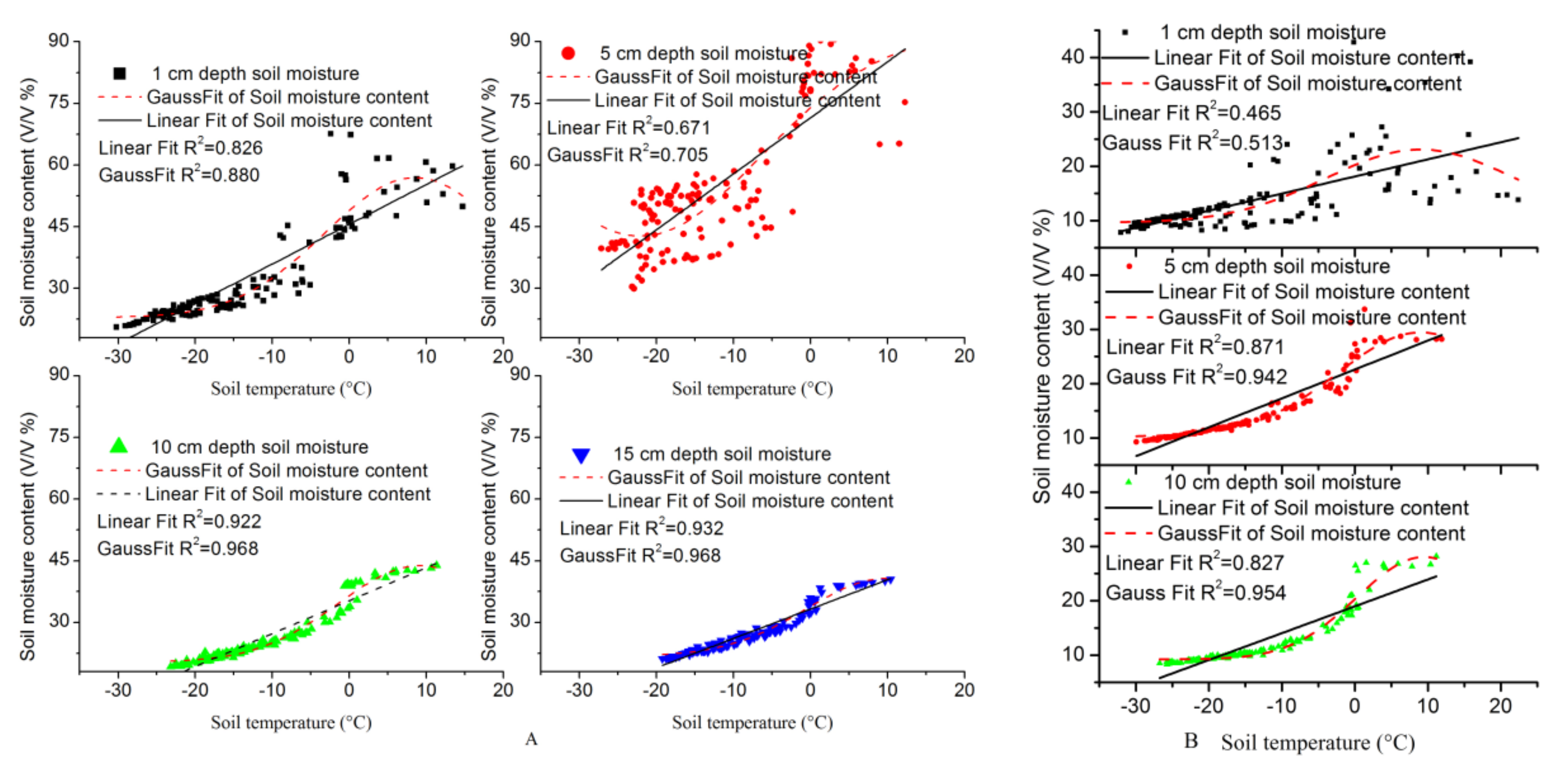
The relationship between soil temperature and soil moisture content in sloping black soil farmland during the freeze–thaw period is shown in Figure 5.
Figure 5A shows abscissa is according to the temperature with time as the axis of freeze–thawing periods from 20 November 2011 to 18 April 2012. Ordinate represent values of volumetric soil moisture contents. Small black solid squares, red solid circles, green solid up triangles, and blue solid down triangles respectively represent soil moisture contents at depths of 1, 5, 10, and 15 cm. The fitted curves plot of the solid lines correspond to a linear distribution of soil moisture contents and soil temperature. The fitted curves plot of the red dashed lines correspond to a Gaussian distribution of soil moisture and soil temperature. Figure 5A,B shows a comparison of Gaussian and linear fits of soil moisture content and temperature during the freeze–thaw periods in sun slope black soil farmland and shady slope black soil farmland, respectively.
As shown in Figure 5A, the linear fit for soil moisture content and temperature at depths of 1, 5, 10, and 15 cm in sunny slope black soil farmland during the freeze–thaw periods has coefficients of determination (R2) of 0.826, 0.671, 0.922, and 0.932, respectively. The Gaussian fit for soil moisture content and temperature at depths of 1, 5, 10, and 15 cm have R2 values of 0.880, 0.705, 0.968, and 0.968, respectively.
In Figure 5B, the linear fit for soil moisture content and temperature at depths of 1, 5, and 10 cm in shady slope black soil farmland during the freeze–thaw periods has R2 values of 0.465, 0.871, and 0.827, respectively. The Gaussian fit for soil moisture content and temperature at depths of 1, 5, and 10 cm has R2 values of 0.513, 0.942, and 0.954, respectively.
It is therefore found that the soil moisture content and soil temperature fit line is consistent with a Gaussian distribution rather than a linear distribution during the freeze–thaw period.
3.3. Soil Moisture Distribution in Freeze–Thaw Period
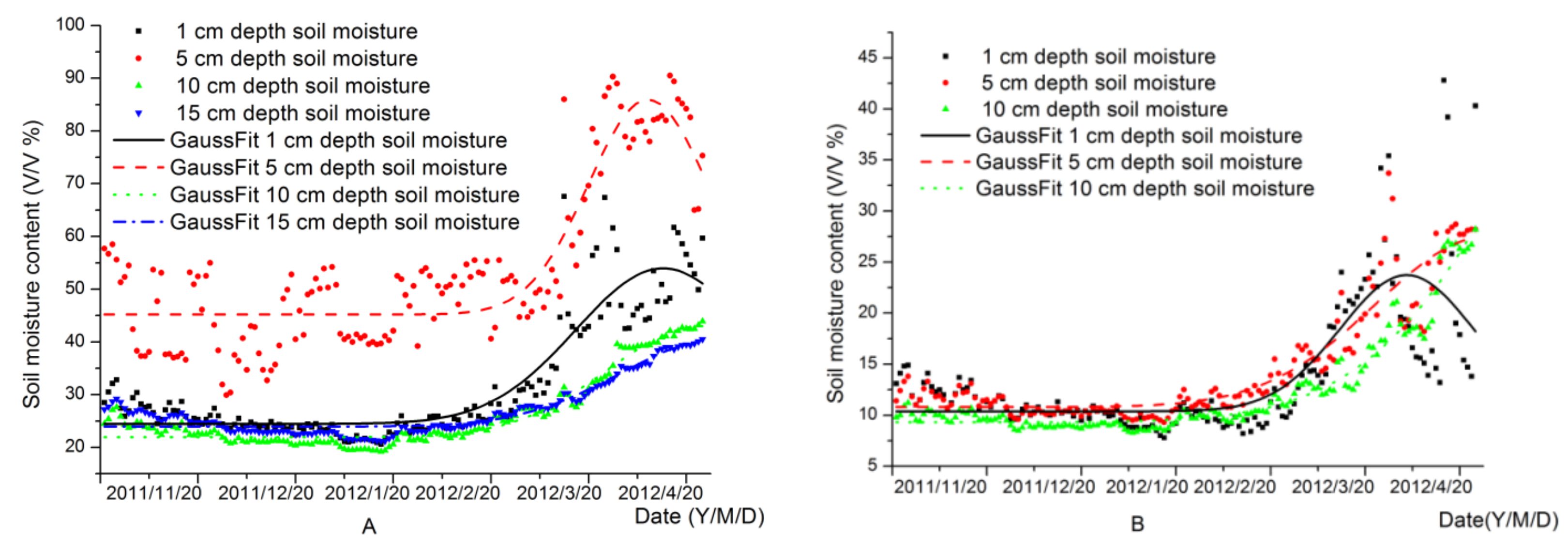
The relationship between soil moisture content and time during the freeze–thaw period in sloping black soil farmland is considered. The distribution of soil moisture content in the sunny and shady slope black soil farmland during the freeze–thaw periods is shown in Figure 6.
Figure 6A shows abscissa is according to the time as the axis of freeze–thawing periods from 20 November 2011 to 18 April 2012. Ordinate represent the values of soil volumetric moisture contents. Small black solid squares, red solid circles, green solid up triangles, and blue solid down triangles respectively represent soil moisture contents at depths of 1, 5, 10, and 15 cm. The fitted curves plot of the black solid lines, red dashed lines, green dotted lines, and blue dashed and dotted lines respectively represent depths of 1, 5, 10, and 15 cm, and correspond to a Gaussian distribution of soil moisture and time. Figure 6A shows a Gaussian fit of soil moisture content and time in sunny slope black soil farmland during the freeze–thaw periods. Figure 6B shows the same as Figure 6A but for the shady slope.
A comparison of curve-fitting parameters of the distributions of soil moisture content is shown in Table 1.
Table 1 show that the soil moisture content and time obeys a Gaussian fit at depths of 1, 5, 10, and 15 cm in sunny slope black soil farmland during the freeze–thaw periods, with R2 values of 0.835, 0.788, 0.948, and 0.910, respectively. The soil moisture content and time obeys a Gaussian fit at depths of 1, 5, and 10 cm in shady slope black soil farmland during the freeze–thaw periods, with R2 values of 0.558, 0.867, and 0.954, respectively.
Therefore, the soil moisture content and time with temperature are in accordance with a Gaussian distribution during the freeze–thaw period.
4. Analysis and Discussion
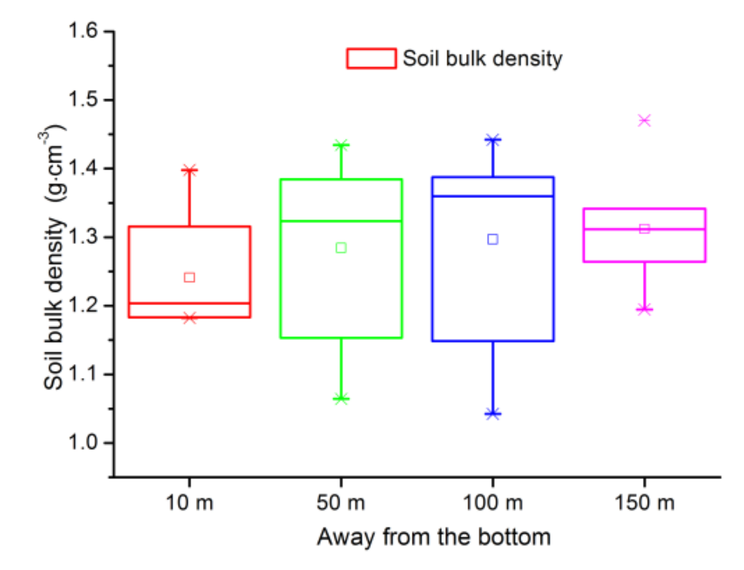
The soil moisture content and soil temperature or time fit line is in accordance with a Gaussian distribution during the freeze–thaw period. In this verification, soil samples were collected from Site 2, which is a 168 m long sloping black soil field, at distances of 10, 50, 100, and 150 m from the bottom of the slope for testing and analysis. During the freeze–thaw periods, surface-soil samples were taken from the sloping black soil farmland at depths of 0–1 cm, 1–5 cm, and 5–10 cm at the same location. At the Site 2 sampling point, in the pre-freezing period, at depths of 10, 50, 100, and 150 m from the bottom of the slope, sampling from the surface of the black soil slope farmland was conducted every 5 to 50 cm depth, and an aluminum box was used to collect the marked soil. In the laboratory, the soil samples were weighed and dried to obtain a soil bulk density measurement chart, as shown in Figure 7.
4.1. Freeze–Thaw Periods Divided into Six Periods
The freeze–thaw periods are abbreviated by F–T. The natural freeze–thaw cycle from late autumn to winter and early spring was divided into six periods: The pre-freezing period (F–Tp), freezing period (F–Tf), early freeze–thaw period (F–Te), mid freeze–thaw period (F–Tm), late freeze–thaw period (F–Tl), and post-thawing period (F–Tpo); which is a function of temperature related (f(t)).
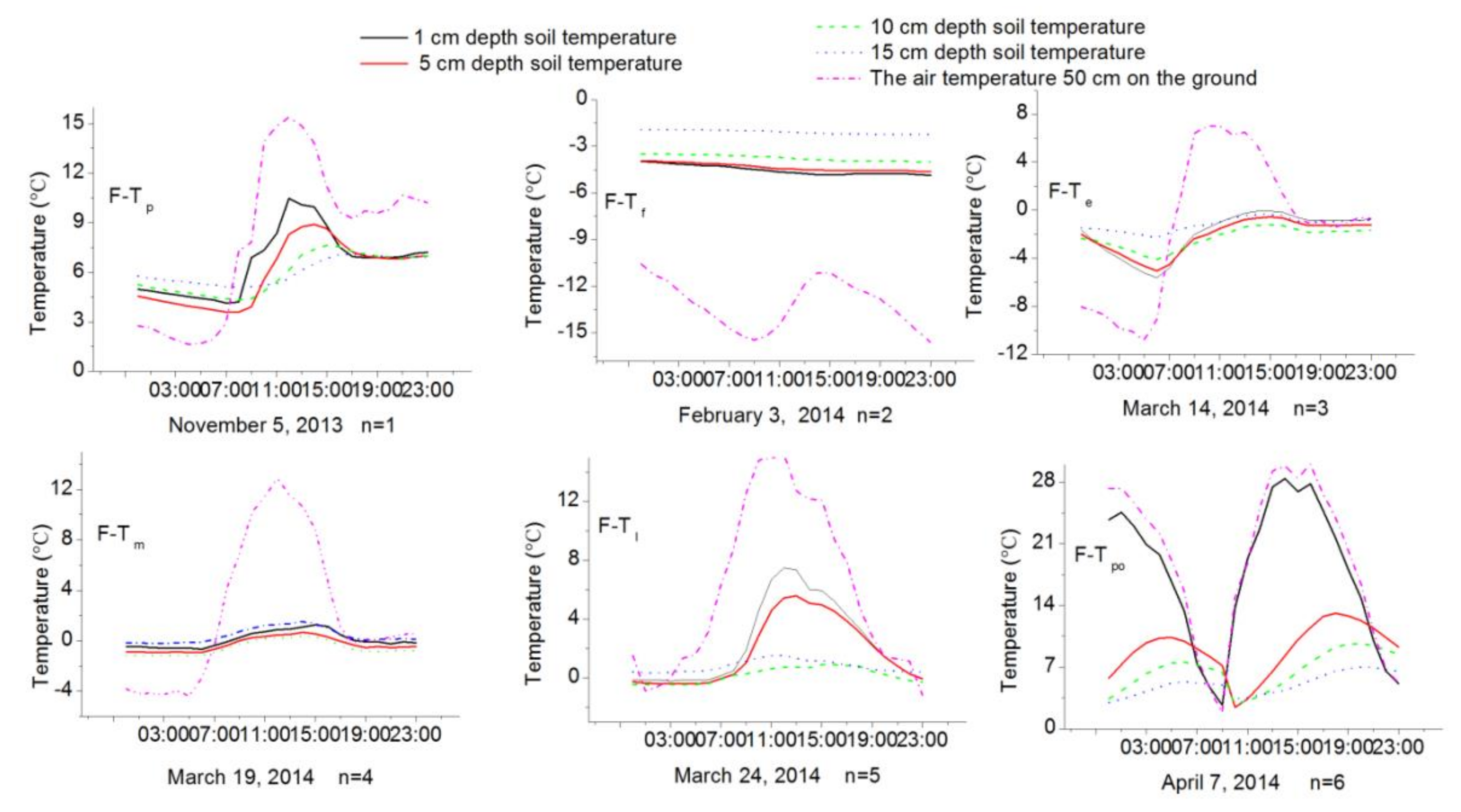
These observations are presented in Table 2 temperature for n freeze–thaw periods (F–Tn), n = 1,2,3,4,5,6, for the observational study. Taking November 2013–April 2014 as an example, the freeze–thaw period is divided into six periods of different air temperatures and different depths of soil temperature. A schematic is shown in Figure 8.
Figure 8 shows the temperatures on the day of sampling at different depths. Time is the x-coordinate, from 00:00 to 23:00 per hour. Temperature is the y-coordinate, including the soil temperature at depths of 1, 5, 10, and 15 cm and the air temperature 50 cm above the ground. The soil moisture contents at the same locations during different periods were tested at depths of 1, 5, and 10 cm, respectively. Sampling was taken at different depths in the different freeze–thaw periods including F–Tp, F–Tf, F–Te, F–Tm, F–Tl, and F–Tpo, according to the soil temperature. Take the freeze–thaw period from October 2013 to April 2014 as an example. F–Tp is from 20 October 2013 to 6 November 2013; F–Tf is from 7 November 2013 to 9 March 2014; F–Te is from 10 March 2014 to 16 March 2014; F–Tm is from 17 March 2014 to 22 March2014; F–Tl is from 23 March 2014 to 25 March 2014; and F–Tpo is after 26 March 2014 to the end of April 2014; which is a function of temperature related. The specific sampling time selection is the F–Tp on 5 November 2013, the F–Tf on 3 February 2014, the F–Te on 14 March 2014, the F–Tm on 19 March 2014, the F–Tl on 24 March2014, and the F–Tpo on 7 April 2014.
4.2. Changes of Soil Moisture Content in Freeze–Thawing Period
Soil samples were collected at depths of 0–1 cm, 1–5 cm, and 5–10 cm, and at distances of 10 m, 50 m, 100 m, and 150 m from the bottom of the sloping black soil farmland in six different periods in time according to the temperature, F–Tn, n = 1,2,3,4,5,6.The soil moisture contents at the same locations during different periods were tested at depths of 0–1 cm, 1–5 cm, and 5–10 cm, respectively. Sampling was performed at different depths in the different freeze–thaw periods including F–Tp, F–Tf, F–Te, F–Tm, F–Tl, and F–Tpo, according to the soil temperature.
4.2.1. Plots of Soil Moisture Contents at the Same Depth
Soil moisture contents at the same depth (0–1 cm, 1–5 cm, 5–10 cm) during different freeze–thaw periods are shown in Figure 9.
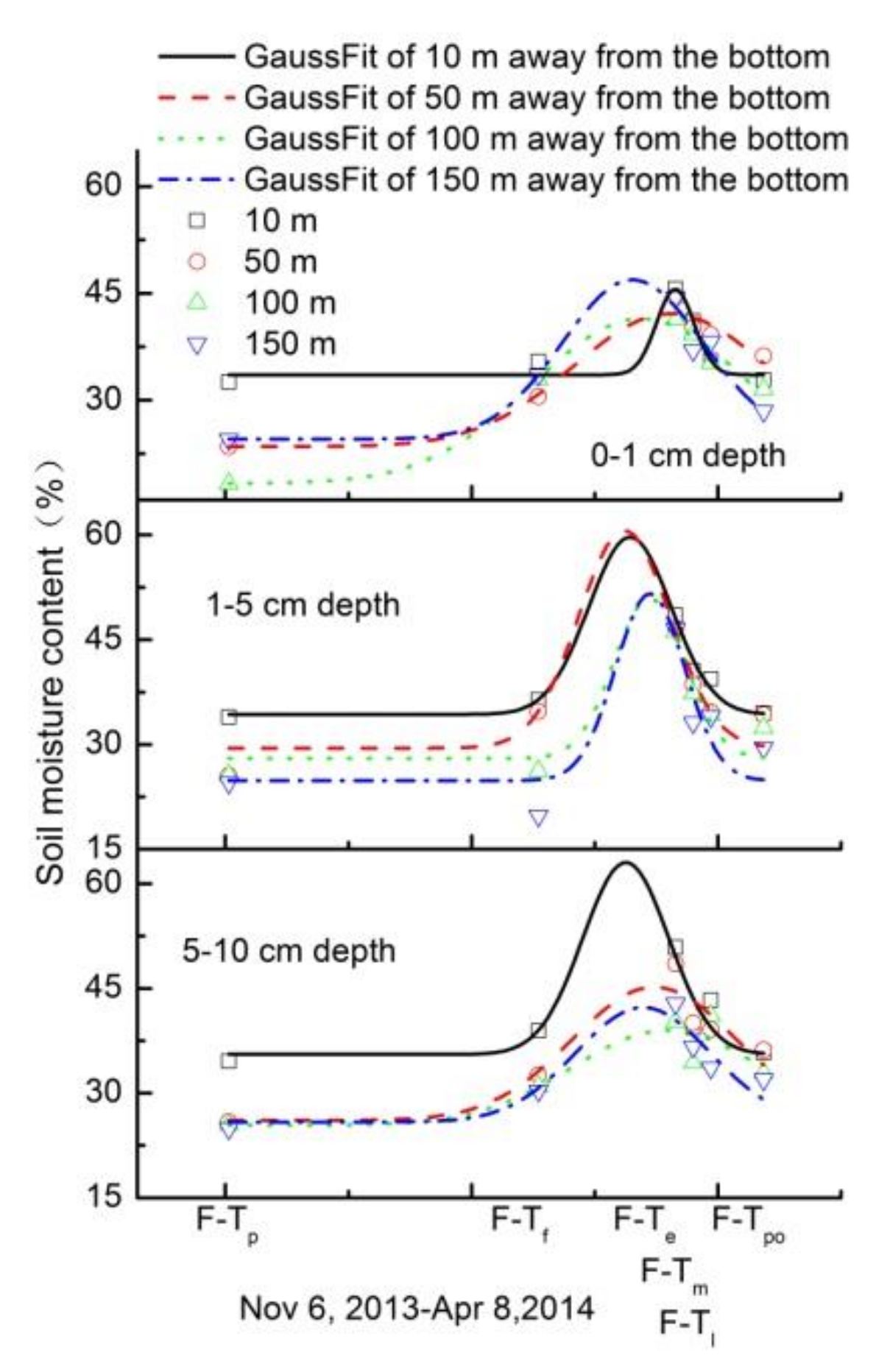
Figure 9 shows abscissa is according to the temperature with time as the axis of freeze–thaw periods from F–Tp, F–Tf, F–Te, F–Tm, F–Tl, and F–Tpo; which is from 6 November 2013 to 8 April 2014. Ordinate represent depths of 0–1 cm, 1–5 cm, and 5–10 cm of soil moisture contents, respectively. Small black open squares represent a distance of 10 m away from the bottom to the base of the 168 m long sloping black soil land, in soil moisture contents at the F–Tp, F–Tf, F–Te, F–Tm, F–Tl, and F–Tpo periods. Open red circles, open green up triangles, and open blue down triangles respectively represent distances of 50, 100, and 150 m away from the bottom in soil moisture contents in the six freeze–thaw periods.
Figure 9 shows soil moisture contents at the same depths during different freeze–thaw periods. The figure shows fitted curves plot of the black solid, red dashed, green dotted, and blue dashed and dotted lines, which respectively correspond to soil moisture contents at distances of 10, 50, 100, and 150 m away from the bottom to the base of the 168 m long sloping black soil land sampling point.
The soil moisture content is influenced by the initial soil moisture content before freezing and snowmelt [11,12,20,23,30,42] in the freeze–thaw period. The soil moisture content decreased slightly after the soil from a depth of 0–1 cm was thawed and increased at depths of 1–5 cm and 5–10 cm compared with the soil moisture content during F–Tp. The maximum soil moisture content at depths of 0–1 cm and 1–5 cm was reached during F–Te (ta > 0 °C at daytime, 1 cm depth ts > 0 °C at noon; ta < 0 °C at night, 1 cm depth ts < 0 ℃ in the morning and at night) due to snowmelt and decreased as the snow melted more with time and temperature. Additionally, the soil moisture content at depths of 0–1 cm, 1–5 cm, and 5–10 cm during F–Tpo was less than that during F–Tl but greater than that during F–Tp. Due to the melting of snow in F–Te, the surface soil moisture content is significantly increased in the F–Te compared to F–Tf, so the soil moisture content fit line is in accordance with Gaussian distribution during the six freeze–thaw periods. The fitted soil moisture content curves conform to Gaussian distributions at the same depths of 0–1 cm, 1–5 cm, and 5–10 cm at different locations in the six freeze–thaw periods.
4.2.2. Soil Moisture Contents Measured at the Same Location
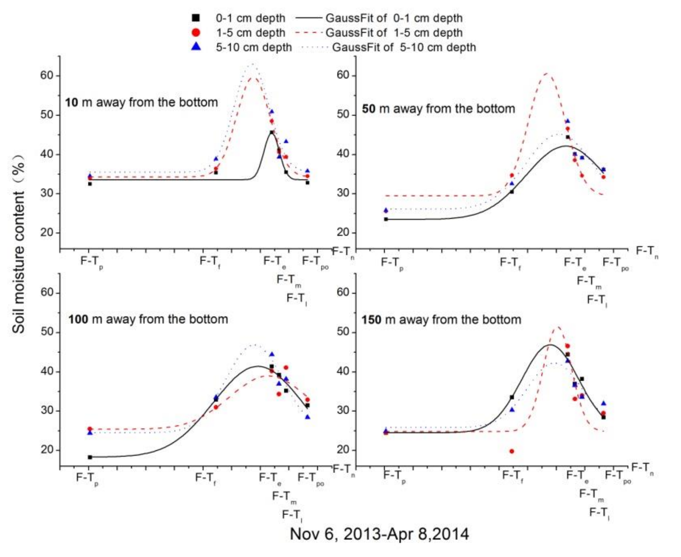
Figure 10 shows plots of soil moisture content during the six different periods according to the temperature. Abscissa is according to the temperature with time as the x-axis showing the freeze–thawing periods F–Tp, F–Tf, F–Te, F–Tm, F–Tl, and F–Tpo; which is from 6 November 2013 to 8 April 2014. Ordinate represent distances of 10, 50, 100, and 150 m away from the bottom to the base of the 168 m long sloping black soil land sampling point of soil moisture contents, respectively. The solid black squares, solid red circles, and blue up triangles correspond to soil moisture contents at depths of 1, 5, and 10 cm, respectively.
Figure 10 shows fitted curves plot of soil moisture contents at the same location during different freeze–thaw periods according to the temperature. The black solid, red dashed, and blue dotted lines correspond to soil moisture contents at depths of 0–1 cm, 1–5 cm, and 5–10 cm, respectively.
At the same location 10 m away from the bottom of the 168 m long sloping black soil land sampling point, and at depths of 0–1 cm, 1–5 cm, and 5–10 cm, the soil moisture content, increased slightly for a while, then increased and finally decreased during the six different periods according to the temperature.
The fitted soil moisture content curves conform to Gaussian distributions at the same location at different depths in the six freeze–thaw periods. From 150 m away from the bottom of the 168 m long sloping black soil land sampling point, 100 m away from the bottom, 50 m away from the bottom, to 10 m away from the bottom, the soil moisture contents gradually increased at depths of 0–1 cm, 1–5 cm, and 5–10 cm during the six freeze–thaw periods. That is to say, in the sloping black soil farmland during the freeze–thaw periods, the soil moisture contents gradually increased from the top to the bottom.
4.3. Verification Analysis of Soil Moisture Contents Distribution
The fitted soil moisture content curves are shown in Figure 9 and Figure 10, whether it is at the same depth different locations in the six freeze–thaw periods or at the same location different depths in the six freeze–thaw periods. The soil moisture content increased slightly for a while from F–Tp to F–Tf, then increased from F–Tf to F–Te. The maximum soil moisture contents occurred during the F–Te period, decreased gradually from F–Tm to F–Tl, and finally decreased during the six different periods according to the temperature. The soil moisture contents at depths of 0–1 cm, 1–5 cm, and 5–10 cm during F–Tpo were lower than those during F–Tl but greater than that during F–Tp.
The soil moisture content increased and then decreased during the six time periods according to the temperature, and the fitted curves follow a Gaussian distribution.
The soil moisture content y follow a Gaussian distribution during the six freeze–thaw periods (F–T)n according to the temperature, as follows:
where y0, A, w, and (F–T)c are parameters. A > 0; soil moisture content offset: y0; the ymax corresponds to center: (F–T)c; soil moisture content variation with time width: w; temperature area: A.
Table 3 shows the curve-fitting of the soil moisture content at distances of 10, 50, 100, and 150 m at depths of 0–1 cm, 1–5 cm, and 5–10 cm, respectively.
At the location 10 m away from the bottom of the 168 m long sloping black soil land sampling point, at depths of 0–1 cm, 1–5 cm, and 5–10 cm during the freeze–thaw period change in six different periods, the Gaussian distribution, when considering the reduced chi-squared statistic, is found to be with average standard deviations of 2.54, 2.31, and 17.79, respectively. The R2 values of 0.905, 0.921, and 0.499 and Prob > F values of 0.0012, 0.001, and 0.0071, respectively, were observed. Prob > F means Probability, less than 0.05 means significant. Additionally, a similar Gaussian distribution was found at the locations 50, 100, and 150 m away from the bottom, at depths of 0–1 cm, 1–5 cm, and 5–10 cm during the freeze–thaw period change in six different periods.
Table 3 shows that the soil moisture contents in the plow layer of black soils at depths of 0–1 cm, 1–5 cm, and 5–10 cm, and at locations 10, 50, 100, and 150 m away from the bottom during the freeze–thaw period, change in six different periods (F–Tp, F–Tf, F–Te, F–Tm, F–Tl, and F–Tpo) and following a Gaussian distribution.
Often, only the conditions before and after the freeze–thaw cycles are considered [2,3,4]. As the data are not fine enough, the daily freeze–thaw cycle is missed every day during the daily data interval. However, the freeze–thaw period can be separated into six periods in time according to the temperature (air and soil): F–Tp, F–Tf, F–Te, F–Tm, F–Tl, and F–Tpo. It is necessary to understand how the soil moisture contents change during the periods between before and after freeze–thaw cycles. Obtaining the soil moisture contents during these periods and understanding the causes of their variations is necessary.
For the results of soil moisture content distribution during the freeze–thaw period in November 2011–April 2012, the soil sample test data of wild slope farmland during the freeze–thaw period from November 2013–April 2014 were used for verification. According to the freeze–thaw cycle, periods F–Tp, F–Tf, F–Te, F–Tm, F–Tl, and F–Tpo, according to the temperature, stratified sampling the soil moisture contents at different locations of 10, 50, 100, and 150 m away from the bottom, respectively. The result is that the soil moisture content at depths of 0–1 cm, 1–5 cm, and 5–10 cm is in accordance with a Gaussian function type distribution. The Gaussian R2 values are 0.742 average soil moisture content at different locations and at different depths. Additionally, from November 2011 to April 2012 in freeze–thaw periods, according to the temperature monitoring of soil moisture sensor, results showed a similar distribution with the Gaussian, and R2 values are 0.837 average of sun and shady soil moisture content at different depths.
In the early spring, when the temperature rises and the snow melts [11,12,20,23,27,30,42], water infiltrates into the soil moisture, the shallow soil moisture increases, the bottom soil freezes and does not melt, and the soil moisture in the freeze–thaw cycle shows a Gaussian distribution, which is consistent with the natural phenomenon of peak soil moisture content.
4.4. Soil Temperature Observed Value Associated with the CMADS-ST Analysis
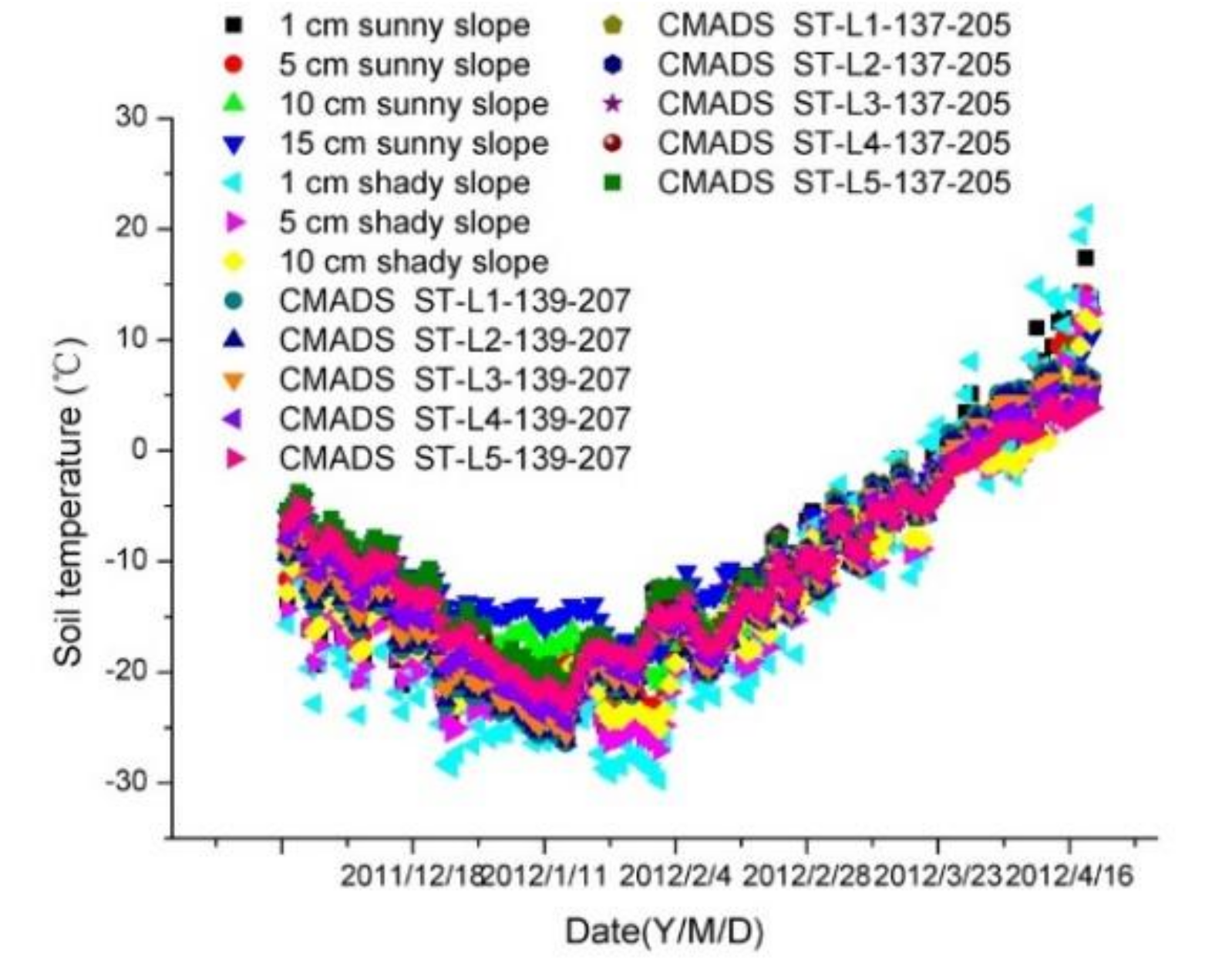
Soil temperature data monitored at Site 1 is a group of every 1 h, divided into four layers (sunny slope) or three layers (shady slope), the time scale from November 2011 to mid-April 2012. We averaged the ground temperature of four daily time periods, namely, 02:00, 08:00, 14:00, and 20:00. The temperature of these four time periods was added and then divided by four. The average daily soil temperature for different layers can be derived. We selected CMADS-ST data of the top five layers (first layer: 0.007 m; second layer: 0.028 m; third layer: 0.062 m; fourth layer: 0.119 m; fifth layer: 0.212 m) for comparison, from the time scale from November 2011 to mid-April 2012, of daily time resolution, from the locations 139–207(45°59′07″ N 128°37′45″ W) and 137–205(45°19′09″ N 127°57′47.7″ W). Soil temperature at Site 1 was correlated with the daily average soil stratification temperature of locations 139–207 and 137–205 CMADS-ST near the observation point. The soil temperature observations from November 2011 to 20 April 2012 was compared with CMADS-ST, as shown in Figure 11.
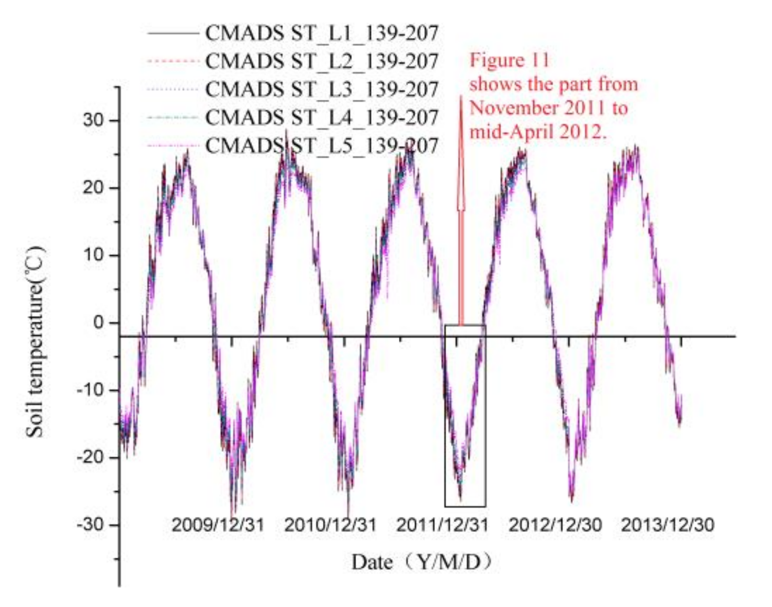
The soil temperature (sunny slope and shady slope) monitoring data of Site 1 were used to analyze the CMADS-ST position points 139–207 and 137–205, respectively, and a linear correlation was found. Soil temperatures (sunny slope and shady slope) and locations 139–207 and 137–205 correlation coefficient R2 value was calculated. The result showed that the sunny slope temperature R2 is between 0.841–0.897, with an average value of 0.880. The mean value between 0.822–0.907 on the shady slope is 0.875; R2 (CMADS-ST for locations 139–207) >R2 (CMADS-ST for locations 137–205). It can be shown that position 139–207 is closer to Site 1 than 137–205. The results of CMADS-ST are in good agreement with the soil temperature measured by the fixed point of Site 1. The practicality of CMADS-ST in black soil slope farmland in the seasonal frozen soil area of the study area is very good. The variation of soil layer temperature in the seasonally frozen ground zone of the longer series CMADS-ST from 1 January 2009 to 31 December 2013 is shown in Figure 12.
The soil temperature data of the sunny slope is more correlated with CMADS-ST, which coincides with the selection of the sunny slope in the wild slope farmland as the test Site 2.The monitored hourly data can be found in the freeze–thaw cycle with the time of day, melting during the day, and freezing at night (refer to Figure 3, the sunny slope soil experienced 39 freeze–thaw cycles, and the shady slope soil 47 cycles); however, the data period is short and the monitoring points are limited; CMADS-ST daily data can only see a large freeze–thaw cycle in the winter of the yearly cycle (refer to Figure 12); however, CMADS has a lot of spatiotemporal data, applied to a wide range of areas with a long series [11,31,33,38,39,40,41,42,43,44,45,46,47,48,49,50,51,52,53,54].Using fixed-point monitoring of refined soil temperature, soil moisture content, precipitation, temperature, nitrogen and phosphorus of nutrients, spatiotemporal CMADS data can be better promoted and applied.
5. Conclusions
This study, which investigated the distribution of soil moisture contents in the surface black soils of seasonal frozen grounds during freeze–thaw periods, lays a foundation for protecting the water resources downstream instead of water carrying soil into the water and the soil resources of sloping black soil farmlands. The soil moisture content in the black soil plow layer changed with temperature during a freeze–thaw period in an area with seasonally frozen grounds.
It was found that the soil moisture content and soil temperature fit line is consistent with Gaussian distribution during the freeze–thaw period. The soil moisture content and time with temperature are in accordance with Gaussian distribution during the freeze–thaw period. This is consistent with the natural phenomenon, that is, the surface soil moisture content in the early spring will peak, whereas in the seasonal frozen ground zone, the temperature increases, the snow melts, the soil surface melts, and the bottom layer freezes.
In this paper, the natural freeze–thaw cycle from late autumn to winter and early spring was divided into six periods according to the temperature: The pre-freezing period (F–Tp), freezing period (F–Tf), early freeze–thaw period (F–Te), mid freeze–thaw period (F–Tm), late freeze–thaw period (F–Tl), and post-thawing period (F–Tpo). According to the soil temperature in the six time periods during the different freeze–thaw periods, it was verified that the soil moisture contents followed a Gaussian distribution at different depths. The maximum surface soil moisture content was reached during the F–Te period, due to air temperature being more than 0 °C at daytime, surface soil temperature more than 0 °C, and deep soil temperature less than 0 °C at noon, and air temperature less than 0 °C at night, surface soil temperature less than0 °C in the morning and at night, start melting snow, which is consistent with the natural phenomenon of early spring peak soil moisture content under temperature rise and snow melt. The soil moisture contents gradually increased from the top to the bottom in sloping black soil farmland during the freeze–thaw period.
The used measurements and analyticalmethods are somewhat valuable as a result of difficult implementation due to the high latitude and freezing climate. These results suggest that further research is necessary on the use of spatiotemporal data CMADS-ST and precipitation datasets of the northeast black soil area for the freeze–thaw cycle prediction of soil moisture content change trend. Based on the relationship between soil temperature and soil moisture content, we can use CMADS-ST data to predict and analyze soil moisture changes in large areas (black soil areas) rather than at several points during freezing and thawing cycles. This study has important significance for decision-making for protecting water and soil environments in black soil slope farmland.
Author Contributions
X.Z. and S.X. conceived and designed the field experiments; X.Z. and T.L. performed the field experiments; P.Q. analyzed the soil sample; G.Q. analyzed the CMADS-ST; X.Z. contributed test site/monitoring instrument/reagents/materials/analysis tools; and X.Z. wrote the paper.
Funding
This study was supported by the National Natural Science Foundation of China (NSFC) (41201264, 51579157, 51779156), the National key research and development plan project of China, (2018YFC0507000), the Heilongjiang Province of China Youth Science Foundation (QC2010099), Heilongjiang Province of China Science and Technology Special Foundation (201606).
Conflicts of Interest
The authors declare no conflict of interest.
References
- Kaighin, A.M.; Alemohammad, S.H.; Akbar, R.; Konings, A.G.; Yueh, S.; Entekhabi, D. The global distribution and dynamics of surface soil moisture. Nat. Geosci. 2017, 10, 100–104. [Google Scholar] [CrossRef]
- Yang, M.; Yao, T.; Gou, X.; Koike, T.; He, Y. The soil moisture distribution, thawing-freezing processes and their effects on the seasonal transition on the Qinghai-Xizang (Tibetan) plateau. J. Asian Earth Sci. 2003, 21, 457–465. [Google Scholar] [CrossRef]
- Li, T.; Shao, M.; Jia, X.; Huang, L. Profile distribution of soil moisture in the gully on the northern Loess Plateau, China. Catena 2018, 171, 460–468. [Google Scholar] [CrossRef]
- Zhang, X.; Zhao, W.; Wang, L.; Liu, Y.; Liu, Y.; Feng, Q. Relationship between soil water content and soil particle size on typical slopes of the Loess Plateau during a drought year. Sci. Total Environ. 2019, 648, 943–954. [Google Scholar] [CrossRef] [PubMed]
- Wei, W.; Feng, X.; Yang, L.; Chen, L.; Feng, T.; Chen, D. The effects of terracing and vegetation on soil moisture retention in a dry hilly catchment in China. Sci. Total Environ. 2019, 647, 1323–1332. [Google Scholar] [CrossRef]
- Yang, L.; Chen, L.; Wei, W. Effects of vegetation restoration on the spatial distribution of soil moisture at the hillslope scale in semi-arid regions. Catena 2015, 124, 138–146. [Google Scholar] [CrossRef]
- Yang, L.; Wei, W.; Chen, L.; Mo, B. Response of deep soil moisture to land use and afforestation in the semi-arid Loess Plateau, China. J. Hydrol. 2012, 475, 111–122. [Google Scholar] [CrossRef]
- Wang, X.; Pan, Y.; Zhang, Y.; Dou, D.; Hu, R.; Zhang, H. Temporal stability analysis of surface and subsurface soil moisture for a transect in artificial revegetation desert area, China. J. Hydrol. 2013, 507, 100–109. [Google Scholar] [CrossRef]
- Zhao, N.; Yu, F.; Li, C.; Wang, H.; Liu, J.; Mu, W. Investigation of Rainfall-Runoff Processes and Soil Moisture Dynamics in Grassland Plots under Simulated Rainfall Conditions. Water 2014, 6, 2671–2689. [Google Scholar] [CrossRef]
- Lazzari, M.; Piccarreta, M.; Manfreda, S. The role of antecedent soil moisture conditions on rainfall-triggered shallow landslides. Nat. Hazards Earth Syst. Sci. Discuss. 2018. [Google Scholar] [CrossRef]
- Meng, X.; Dan, L.; Liu, Z. Energy balance-based SWAT model to simulate the mountain snowmelt and runoff—Taking the application in Juntanghu watershed (China) as an example. J. Mt. Sci. 2015, 12, 368–381. [Google Scholar] [CrossRef]
- Wang, Y.; Meng, X. Snowmelt runoff analysis under generated climate change scenarios for the Juntanghu River basin in Xinjiang, China. Tecnol. Cienc. Agua 2016, 7, 41–54. [Google Scholar]
- Ala, M.; Ya, L.; Anzhi, W.; Cunyang, N. Characteristics of soil freeze–thaw cycles and their effects on water enrichment in the rhizosphere. Geoderma 2016, 264, 132–139. [Google Scholar]
- Chen, S.; Ouyang, W.; Hao, F.; Zhao, X. Combined impacts of freeze–thaw processes on paddy land and dry land in Northeast China. Sci. Total Environ. 2013, 456, 24–33. [Google Scholar] [CrossRef] [PubMed]
- Kelln, C.; Barbour, S.L.; Qualizza, C. Controls on the spatial distribution of soil moisture and solute transport in a sloping reclamation cover. Can. Geotech. J. 2008, 45, 351–366. [Google Scholar] [CrossRef]
- Messiga, A.J.; Ziadi, N.; Morel, C.; Parent, L.E. Soil phosphorus availability in no-till versus conventional tillage following freezing and thawing cycles. Can. J. Soil Sci. 2010, 90, 419–428. [Google Scholar] [CrossRef]
- Lei, Z.; Shang, S.; Yang, S.; Wang, Y.; Zhao, D. Simulation on phreatic evaporation during soil freezing. J. Hydraul. Eng. 1999, 6, 8–12. [Google Scholar]
- Harlan, R.L. Analysis of coupled heat-fluid transport in partially frozen soil. Water Resour. Res. 1973, 9, 1314–1323. [Google Scholar] [CrossRef]
- Zhang, H.; Chen, X.; Hu, Y. Freeze under the conditions of unsaturated soil, water, heat, and solute coupled transport modeling. Yangtze River 2009, 40, 78–80. [Google Scholar]
- Warrach, K.; Mengelkamp, H.T.; Raschke, E. Treatment of frozen soil and snow cover in the land surface model SEWAB. Theor. Appl. Climatol. 2001, 69, 23–37. [Google Scholar] [CrossRef]
- Sinha, T.; Cherkauer, K.A. Time series analysis of soil freeze and thaw processes in Indiana. J. Hydrometeorol. 2008, 9, 936–950. [Google Scholar] [CrossRef]
- Zhang, X.; Sun, S. The impact of soil freezing/thawing processes on water and energy balances. Adv. Atmos. Sci. 2011, 28, 169–177. [Google Scholar] [CrossRef]
- Wei, D.; Chen, X.; Wang, T. Migration of different snow cover conditions, soil freezing and soil water. J. Anhui Agric. Sci. 2007, 12, 3570–3572. [Google Scholar]
- Liu, T.; Huang, Y.; Zhang, R.; Li, J. Experiment study on the law of thermal motion of water of soil freeze-thaw on the black land. In Proceedings of the Second International Conference on Mechanic Automation and Control Engineering Institute of Electrical and Electronics Engineers, Inner Mongolia, China, 15–17 July 2011. [Google Scholar]
- Li, R.; Shi, H.; Flerchinger, G.N.; Akae, T.; Wang, C. Simulation of freezing and thawing soils in inner Mongolia Hetao irrigation district, China. Geoderma 2012, 173, 28–33. [Google Scholar] [CrossRef]
- French, H.K.; van der Zee, S.E. Improved management of winter operations to limit subsurface contamination with degradable deicing chemicals in cold regions. Environ. Sci. Pollut. Res. 2014, 21, 8897–8913. [Google Scholar] [CrossRef] [PubMed]
- Zhao, X.; Xu, S.; Liu, Z. Study on Freeze-Thaw erosion lead to black soil and agricultural non-point source pollution. In 8th China Water Forum; China Water & Power Press: Beijing, China, 2010; pp. 268–272. [Google Scholar]
- Zhao, X.; Liu, T.; Xu, S.; Liu, Z. Freezing-thawing process and soil moisture migration within the black soil plow layer in seasonally frozen ground regions. J. Glaciol. Geocryol. 2015, 37, 233–240. [Google Scholar]
- Zhao, X.; Liu, Z.; Xu, S.; Liu, T. Study of the black soil plow layer moisture changing with temperature in freeze-thaw cycle period in the seasonal frozen soil regions. J. Glaciol. Geocryol. 2015, 37, 931–939. [Google Scholar]
- Zhao, X.; Xu, S.; Li, M. Freeze-Thaw lead to black soil erosion and non-point source pollution preferences: Alterable fuzzy optimum model of semi-structural decision applied. World Hydrol. 2015, 272, 14–18. [Google Scholar]
- Meng, X.; Wang, H.; Wu, Y.; Long, A.; Wang, J.; Shi, C.; Ji, X. Investigating spatiotemporal changes of the land surface processes in Xinjiang using high-resolution CLM3.5 and CLDAS: Soil temperature. Sci. Rep. 2017, 7, 13286. [Google Scholar] [CrossRef] [PubMed]
- Nayak, H.P.; Osuri, K.K.; Sinha, P.; Nadimpalli, R.; Mohanty, U.C.; Chen, F.; Rajeevan, M.; Niyogi, D. High-resolution gridded soil moisture and soil temperature datasets for the Indian monsoon region. Sci. Data 2018, 5, 180264. [Google Scholar] [CrossRef]
- Yang, K.; Zhang, J. Evaluation of reanalysis datasets against observational soil temperature data over China. Clim. Dyn. 2018, 50, 317–337. [Google Scholar] [CrossRef]
- Davtian, N.; Menot, G.; Bard, E.; Poulenard, J.; Podwojewski, P. Consideration of soil types for the calibration of molecular proxies for soil pH and temperature using global soil datasets and Vietnamese soil profiles. Org. Geochem. 2016, 101, 140–153. [Google Scholar] [CrossRef]
- Gómez, I.; Caselles, V.; Estrela, M.J.; Niclòs, R. Impact of Initial Soil Temperature Derived from Remote Sensing and Numerical Weather Prediction Datasets on the Simulation of Extreme Heat Events. Remote Sens. 2016, 8, 589. [Google Scholar] [CrossRef]
- Ambadan, J.T.; Berg, A.A.; Merryfield, W.J.; Lee, W. Influence of snowmelt on soil moisture and on near surface air temperature during winter–spring transition season. Clim. Dyn. 2018, 51, 1295–1309. [Google Scholar] [CrossRef]
- Meng, X.; Wang, H.; Lei, X.; Cai, S.; Wu, H. Hydrological Modeling in the Manas River Basin Using Soil and Water Assessment Tool Driven by CMADS. Teh. Vjesn. 2017, 24, 525–534. [Google Scholar]
- Meng, X.; Wang, H.; Cai, S.; Zhang, X.; Leng, G.; Lei, X.; Shi, C.; Liu, S.; Shang, Y. The China Meteorological Assimilation Driving Datasets for the SWAT Model (CMADS) Application in China: A Case Study in Heihe River Basin. Preprints 2016, 120091. [Google Scholar] [CrossRef]
- Shi, C.; Xie, Z.; Qian, H.; Liang, M.; Yang, X. China land soil moisture EnKF data assimilation based on satellite remote sensing data. China Earth Sci. 2011, 54, 1430. [Google Scholar] [CrossRef]
- Stamnes, K.; Tsay, S.C.; Wiscombe, W.; Jayaweera, K. Numerically stable algorithm for discrete-ordinate method radiative transfer in multiple scattering and emitting layered media. Appl. Opt. 1988, 27, 2502–2509. [Google Scholar] [CrossRef] [PubMed]
- Meng, X. Spring Flood Forecasting Based on the WRF-TSRM mode. Teh. Vjesn. 2018, 25, 27–37. [Google Scholar]
- Zhao, F.; Wu, Y. Parameter Uncertainty Analysis of the SWAT Model in a Mountain Loess Transitional Watershed on the Chinese Loess Plateau. Water 2018, 10, 690. [Google Scholar] [CrossRef]
- Liu, J.; Shanguan, D.; Liu, S.; Ding, Y. Evaluation and Hydrological Simulation of CMADS and CFSR Reanalysis Datasets in the Qinghai Tibet Plateau. Water 2018, 10, 513. [Google Scholar] [CrossRef]
- Cao, Y.; Zhang, J.; Yang, M. Application of SWAT Model with CMADS Data to Estimate Hydrological Elements and Parameter Uncertainty Based on SUFI-2 Algorithm in the Lijiang River Basin, China. Water 2018, 10, 742. [Google Scholar] [CrossRef]
- Shao, G.; Guan, Y.; Zhang, D.; Yu, B.; Zhu, J. The Impacts of Climate Variability and Land Use Change on Streamflow in the Hailiutu River Basin. Water 2018, 10, 814. [Google Scholar] [CrossRef]
- Zhou, S.; Wang, Y.; Chang, J.; Guo, A.; Li, Z. Investigating the Dynamic Influence of Hydrological Model Parameters on Runoff Simulation Using Sequential Uncertainty Fitting-2-Based Multilevel-Factorial-Analysis Method. Water 2018, 10, 1177. [Google Scholar] [CrossRef]
- Qin, G.; Liu, J.; Wang, T.; Xu, S.; Su, G. An Integrated Methodology to Analyze the Total Nitrogen Accumulation in a Drinking Water Reservoir Based on the SWAT Model Driven by CMADS: A Case Study of the Biliuhe Reservoir in Northeast China. Water 2018, 10, 1535. [Google Scholar] [CrossRef]
- Guo, B.; Zhang, J.; Xu, T.; Croke, B.; Jakeman, A.; Song, Y.; Yang, Q.; Lei, X.; Liao, W. Applicability Assessment and Uncertainty Analysis of Multi-Precipitation Datasets for the Simulation of Hydrologic Models. Water 2018, 10, 1611. [Google Scholar] [CrossRef]
- Dong, N.; Yang, M.; Meng, X.; Liu, X.; Wang, Z.; Wang, H.; Yang, C. CMADS-Driven Simulation and Analysis of Reservoir Impacts on the Streamflow with a Simple Statistical Approach. Water 2018, 11, 178. [Google Scholar] [CrossRef]
- Vu, T.; Li, L.; Jun, K. Evaluation of Multi-Satellite Precipitation Products for Streamflow Simulations: A Case Study for the Han River Basin in the Korean Peninsula, East Asia. Water 2018, 10, 642. [Google Scholar] [CrossRef]
- Meng, X.; Wang, H. Significance of the China Meteorological Assimilation Driving Data sets for the SWAT Model (CMADS) of East Asia. Water 2017, 9, 765. [Google Scholar] [CrossRef]
- Meng, X.; Wang, H.; Shi, C.; Wu, Y.; Ji, X. Establishment and Evaluation of the China Meteorological Assimilation Driving Datasets for the SWAT Model (CMADS). Water 2018, 10, 1555. [Google Scholar] [CrossRef]
- Meng, X. Simulation and spatiotemporal pattern of air temperature and precipitation in Eastern Central Asia using RegCM. Sci. Rep. 2018, 8, 3639. [Google Scholar] [CrossRef] [PubMed]
- Tian, Y.; Zhang, K.; Xu, Y.; Gao, X.; Wang, J. Evaluation of Potential Evapo-transpiration Based on CMADS Reanalysis Dataset over China. Water 2018, 10, 1126. [Google Scholar] [CrossRef]
Figure 1.
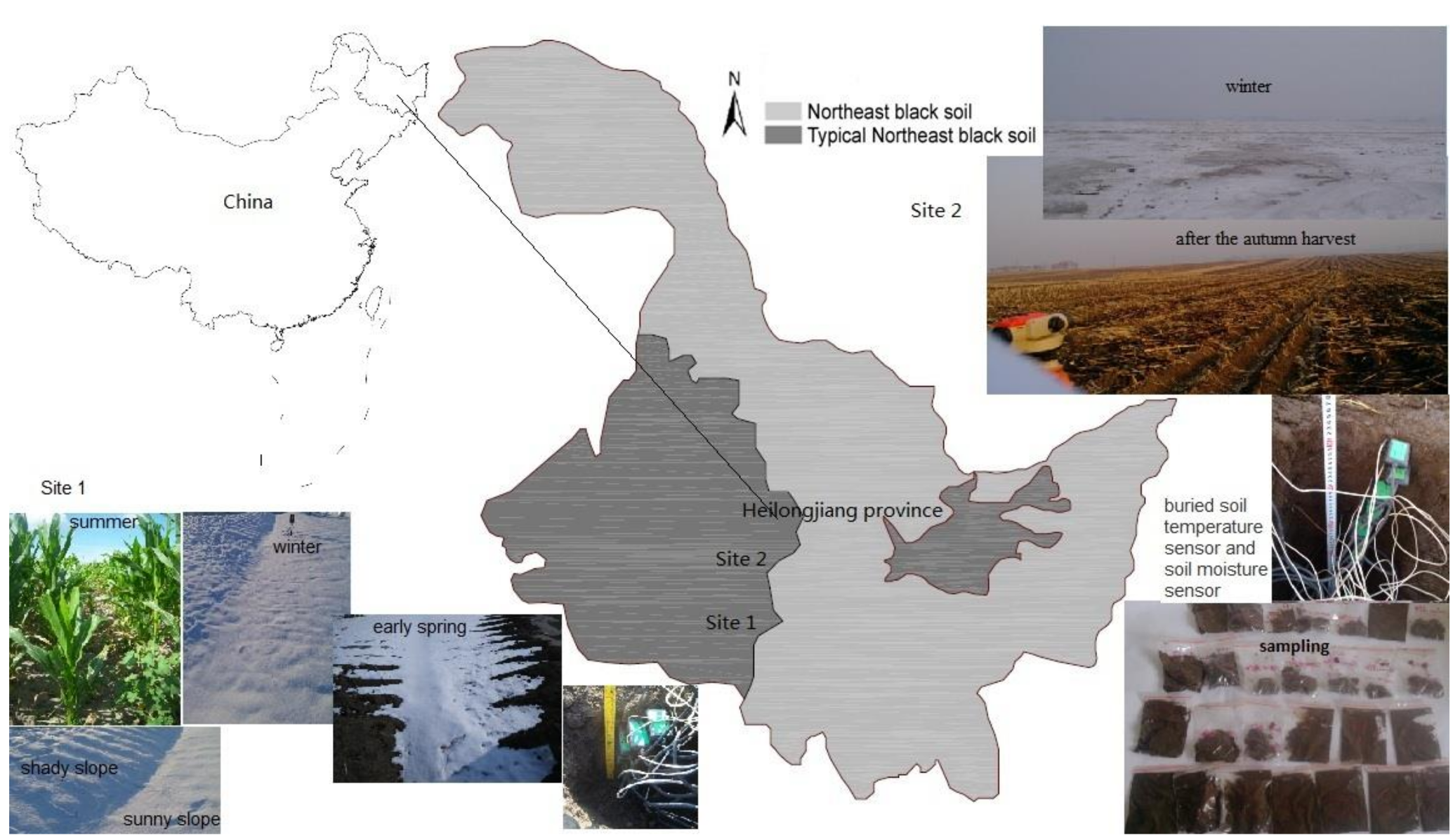
Map of the observation point locations and site case diagram, Heilongjiang Province, Northeastern China. Light gray indicates the northeast black soil zone and dark gray indicates the typical northeast black soil zone. Site 1—corn is grown in summer, snow cover in winter, shady slope and sunny slope obvious, early spring snowmelt. Site 2—using the level gauge to measure the height of black soil slope farmland after autumn harvest, buried soil temperature sensor and soil moisture sensor, snow in winter, black soil sampling.
Figure 1.
Map of the observation point locations and site case diagram, Heilongjiang Province, Northeastern China. Light gray indicates the northeast black soil zone and dark gray indicates the typical northeast black soil zone. Site 1—corn is grown in summer, snow cover in winter, shady slope and sunny slope obvious, early spring snowmelt. Site 2—using the level gauge to measure the height of black soil slope farmland after autumn harvest, buried soil temperature sensor and soil moisture sensor, snow in winter, black soil sampling.

Figure 2.
Moisture contents and soil temperature distribution at different depths during the freeze–thaw period. (A) Sunny slope black soil farmland; (B) shady slope black soil farmland. Solid symbols (squares, circle, up triangle, down triangle) represent soil moisture and open symbols represent soil temperature. Different colors represent soil moisture content at different depths of soil temperature. The abscissa is always the same and the ordinate is different each time.

Figure 3.
Variations of soil temperature in the black soil plow layer during the soil thawing period at different underground depths. (A) is sunny slope black soil farmland, soil temperature recorded hourly, 39 freeze–thaw cycles in the freeze–thaw period; (B) is shady slope black soil farmland, 47 freeze–thaw cycles in the freeze–thaw period. Data are from the period 26 February–20 April 2012.

Figure 4.
Moisture content and precipitation during the freeze–thaw periods. (A) is sunny slope black soil farmland; (B) is shady slope black soil farmland.
Figure 4.
Moisture content and precipitation during the freeze–thaw periods. (A) is sunny slope black soil farmland; (B) is shady slope black soil farmland.

Figure 5.
Comparison of Gaussian and linear fits of soil moisture content and temperature during the freeze–thaw periods. (A) is in sunny slope black soil farmland; (B) is in shady slope black soil farmland. The black solid line represents linear fit and the red dashed line represents Gaussian fit.
Figure 5.
Comparison of Gaussian and linear fits of soil moisture content and temperature during the freeze–thaw periods. (A) is in sunny slope black soil farmland; (B) is in shady slope black soil farmland. The black solid line represents linear fit and the red dashed line represents Gaussian fit.

Figure 6.
Distribution of soil moisture content during the freeze–thaw periods. (A) is in sunny slope black soil farmland; (B) is in shady slope black soil farmland.
Figure 6.
Distribution of soil moisture content during the freeze–thaw periods. (A) is in sunny slope black soil farmland; (B) is in shady slope black soil farmland.

Figure 7.
Soilbulk density measurement chart.

Figure 8.
Temperatures on the day of sampling at different depths. Freeze–thaw periods are divided into six periods, including the pre-freezing period (F–Tp), freezing period (F–Tf), early freeze–thaw period (F–Te), mid freeze–thaw period (F–Tm), late freeze–thaw period (F–Tl), and post-thawing period (F–Tpo), according to the soil temperature.

Figure 9.
Distribution of soil moisture content at the same depth during the freeze–thaw periods.

Figure 10.
Plots of the soil moisture contents at the same location during the freeze–thaw periods.

Figure 11.
Comparison of observed soil temperature with the China meteorological assimilation driving datasets for the soil and water assessment tool (SWAT) model–soil temperature (CMADS-ST) (November 2011 to mid-April 2012).
Figure 11.
Comparison of observed soil temperature with the China meteorological assimilation driving datasets for the soil and water assessment tool (SWAT) model–soil temperature (CMADS-ST) (November 2011 to mid-April 2012).

Figure 12.
Seasonal variation of soil layer temperature with the CMADS-ST in seasonally frozen ground zone between 1 January 2009 and 31 December 2013 for CMADS-ST locations 139–207. The black box section shows some soil layer temperature data from November 2011 to mid-April 2012, as shown in Figure 11.


Table 1.
Curve-fitting parameters of the distribution of soil moisture content, 20 November 2011–18 April 2012.
Table 1.
Curve-fitting parameters of the distribution of soil moisture content, 20 November 2011–18 April 2012.
| Model | Gaussian | ||||||||
|---|---|---|---|---|---|---|---|---|---|
| Equation | |||||||||
| Sunny slope | Depth | 1 cm | 5 cm | 10 cm | 15 cm | ||||
| Reduced Chi-Sqr | 22.52 | 52.48 | 2.5 | 2.4 | |||||
| R2 | 0.835 | 0.788 | 0.948 | 0.91 | |||||
| Prob > F | 0.0001 | 0.0001 | 0.0001 | 0.0001 | |||||
| Parameter | Value | Standard Error | Value | Standard Error | Value | Standard Error | Value | Standard Error | |
| y0 | 24.46 | 0.53 | 45.22 | 0.74 | 21.93 | 0.18 | 23.93 | 0.17 | |
| xc | 138.29 | 2.22 | 134.59 | 1.07 | 148.18 | 2.57 | 152.63 | 4.79 | |
| w | 42.78 | 3.98 | 29.31 | 2.41 | 46.92 | 3.28 | 49.92 | 5.37 | |
| A | 1581.8 | 159.9 | 1496.6 | 114.2 | 1240.6 | 124 | 1039.1 | 182.8 | |
| Shady slope | Depth | 1 cm | 5 cm | 10 cm | |||||
| Reduced Chi-Sqr | 18 | 4.4 | 1.14 | ||||||
| R2 | 0.558 | 0.867 | 0.954 | ||||||
| Prob > F | 0.0001 | 0.0001 | 0.0001 | ||||||
| Parameters | Value | Standard Error | Value | Standard Error | Value | Standard Error | |||
| y0 | 10.38 | 0.46 | 10.8 | 0.25 | 9.31 | 0.13 | |||
| xc | 130.54 | 1.86 | 151.28 | 6.02 | 204.25 | 26.85 | |||
| w | 33.8 | 4.37 | 56.95 | 7.18 | 82.07 | 15.14 | |||
| A | 565.5 | 69.2 | 1193 | 233.8 | 5023.9 | 3807.4 | |||
Note: Where y0, A, w, and xc are parameters. A > 0; offset: y0; center: xc; width: w; area: A. Prob > F: Probability is greater than F test (Also called Homogeneity test of variance).
Table 2.
Freeze–thaw periods divided into six periods.
| n | Periods | F–Tn = f(t) | Season | ta | ts |
|---|---|---|---|---|---|
| 1 | Pre-freezing period | F–T1 = F–TP = f(t) | After the autumn harvest to winter | >0 °C | >0 °C (all day) |
| 2 | Freezing period | F–T2 = F–Tf = f(t) | Winter | <0 °C | <0 °C |
| 3 | Early freeze–thaw period | F–T3 = F–Te = f(t) | Early spring | >0 °C at daytime | 1 cm depth >0 °C at noon |
| <0 °C at night | 1 cm depth <0 °C in the morning and at night | ||||
| 4 | Mid freeze–thaw period | F–T5 = F–Tl = f(t) | Early-mid spring | >0 °C at daytime | >0 °C at daytime |
| <0 °C at night | <0 °C at night | ||||
| 5 | Late freeze–thaw period | F–T5 = F–Tl = f(t) | Mid spring | >0 °C at daytime | >0 °C at daytime |
| >0 °C during night (most of the time, and occasionally below 0 °C) | ≈0 °C ↓↑ at night | ||||
| 1 cm depth >0 ℃ | |||||
| 5 cm depth <0 °C at night | |||||
| 6 | Post-thawing period | F–T6 = F–TPo = f(t) | Late spring | >0 °C | >0 °C at depths of 1 cm, 5 cm, to 10 cm and 15 cm |
Notes: The freeze–thaw periods are abbreviated by F−T, which is a function of temperature related (f(t)); F–Tn = f(t), n = 1,2,3,4,5,6; >is more than, < is less than, ≈ is about equal, ↓↑ is up and down fluctuating; t is short for temperature, including air temperature and soil temperature, ta is short for air temperature, and ts is short for soil temperature.
Table 3.
Curve-fitting parameters of the soil moisture content.
| Model | Gaussian | ||||||
|---|---|---|---|---|---|---|---|
| Equation | |||||||
| Location | Depth | 0–1 cm | 1–5 cm | 5–10 cm | |||
| 10 m away from the bottom | Reduced Chi-Sqr | 2.54 | 2.31 | 17.79 | |||
| R2 | 0.905 | 0.921 | 0.499 | ||||
| Prob > F | 0.0012 | 0.001 | 0.0071 | ||||
| Parameters | Value | Standard Error | Value | Standard Error | Value | Standard Error | |
| y0 | 33.57 | 0.92 | 34.3 | 1.12 | 35.56 | 3.12 | |
| (F–T)c | 127.86 | 3.7 | 115.01 | 2.16 | 113.83 | 4.47 | |
| W | 10.6 | 5.87 | 23.41 | 3.42 | 24.38 | 9.37 | |
| A | 160.1 | 100.9 | 745.2 | 199.8 | 840.4 | 527.7 | |
| 50 m away from the bottom | Reduced Chi-Sqr | 5.38 | 18.15 | 17.21 | |||
| R2 | 0.905 | 0.612 | 0.703 | ||||
| Prob > F | 0.0027 | 0.0092 | 0.0081 | ||||
| Parameters | Value | Standard Error | Value | Standard Error | Value | Standard Error | |
| y0 | 23.49 | 2.32 | 29.49 | 3.23 | 26.11 | 4.14 | |
| (F–T)c | 126.54 | 4.35 | 113.43 | 3.47 | 121.97 | 6.31 | |
| W | 55.04 | 9.94 | 25.95 | 8.64 | 46.72 | 14.33 | |
| A | 1286.6 | 326.8 | 1013.7 | 479.2 | 1118.1 | 497.2 | |
| 100 m away from the bottom | Reduced Chi-Sqr | 2.91 | 15.76 | 15.69 | |||
| R2 | 0.956 | 0.73 | 0.55 | ||||
| Prob > F | 0.0017 | 0.0089 | 0.0087 | ||||
| Parameters | Value | Standard Error | Value | Standard Error | Value | Standard Error | |
| y0 | 18.31 | 1.72 | 27.99 | 3.02 | 25.43 | 3.96 | |
| (F–T)c | 118.3 | 2.39 | 120.6 | 32.1 | 125.61 | 9.92 | |
| W | 61.83 | 7.86 | 20.13 | 30.46 | 54.31 | 22.84 | |
| A | 1791.3 | 265.9 | 579.2 | 1837.6 | 923.5 | 547.1 | |
| 150 m away from the bottom | Reduced Chi-Sqr | 6.69 | 38.79 | 10.76 | |||
| R2 | 0.87 | 0.544 | 0.705 | ||||
| Prob > F | 0.0036 | 0.0245 | 0.0063 | ||||
| Parameters | Value | Standard Error | Value | Standard Error | Value | Standard Error | |
| y0 | 24.52 | 2.51 | 24.83 | 4.58 | 25.87 | 3.2 | |
| (F–T)c | 115.75 | 2.7 | 120.73 | 49.38 | 118.72 | 5.25 | |
| W | 39.85 | 8.15 | 19.6 | 45.74 | 38.11 | 12.26 | |
| A | 1117.9 | 254.2 | 657.3 | 3268.8 | 784.4 | 334.2 | |
© 2019 by the authors. Licensee MDPI, Basel, Switzerland. This article is an open access article distributed under the terms and conditions of the Creative Commons Attribution (CC BY) license (http://creativecommons.org/licenses/by/4.0/).
Share and Cite
MDPI and ACS Style
Zhao, X.; Xu, S.; Liu, T.; Qiu, P.; Qin, G. Moisture Distribution in Sloping Black Soil Farmland during the Freeze–Thaw Period in Northeastern China. Water 2019, 11, 536. https://doi.org/10.3390/w11030536
AMA Style
Zhao X, Xu S, Liu T, Qiu P, Qin G. Moisture Distribution in Sloping Black Soil Farmland during the Freeze–Thaw Period in Northeastern China. Water. 2019; 11(3):536. https://doi.org/10.3390/w11030536
Chicago/Turabian StyleZhao, Xianbo, Shiguo Xu, Tiejun Liu, Pengpeng Qiu, and Guoshuai Qin. 2019. "Moisture Distribution in Sloping Black Soil Farmland during the Freeze–Thaw Period in Northeastern China" Water 11, no. 3: 536. https://doi.org/10.3390/w11030536
Note that from the first issue of 2016, this journal uses article numbers instead of page numbers. See further details here.