Future Hydrological Drought Risk Assessment Based on Nonstationary Joint Drought Management Index

Abstract

As the environment changes, the stationarity assumption in hydrological analysis has become questionable. If nonstationarity of an observed time series is not fully considered when handling climate change scenarios, the outcomes of statistical analyses would be invalid in practice. This study established bivariate time-varying copula models for risk analysis based on the generalized additive models in location, scale, and shape (GAMLSS) theory to develop the nonstationary joint drought management index (JDMI). Two kinds of daily streamflow data from the Soyang River basin were used; one is that observed during 1976–2005, and the other is that simulated for the period 2011–2099 from 26 climate change scenarios. The JDMI quantified the multi-index of reliability and vulnerability of hydrological drought, both of which cause damage to the hydrosystem. Hydrological drought was defined as the low-flow events that occur when streamflow is equal to or less than Q80 calculated from observed data, allowing future drought risk to be assessed and compared with the past. Then, reliability and vulnerability were estimated based on the duration and magnitude of the events, respectively. As a result, the JDMI provided the expected duration and magnitude quantities of drought or water deficit.

1. Introduction

The stationarity assumption in traditional hydrological analysis indicates that statistical characteristics of data do not vary over time. However, handling hydrological data becomes more challenging because the effects of global climate change have led to the nonstationarity of hydrometeorological variables. If the nonstationarity of hydrometeorological variables is not fully considered, the statistical results would be invalid in practice [1], especially when using climate change scenarios.

Therefore, many researchers have been focusing on identifying the time-varying characteristics. Nonstationarity can be simply checked by the trend test and change point analysis [2,3,4], however, the most common way of accounting for nonstationarity is the time-varying moment method [5]. This method assumes that the distribution parameters are functions of time, although variables of interest remain the same [6,7,8,9]. Rigby and Stasinopoulos [10] developed generalized additive models in location, scale, and shape (GAMLSS). GAMLSS overcomes the limitations of generalized linear models (GLM) and generalized additive models (GAM), by expanding the types of distributions and their parameters. Furthermore, it allows modeling of not only the mean and location but also skewness and kurtosis, and introduces the parametric, semi-parametric, non-parametric, or random effect terms of explanatory variables.

The GAMLSS framework has been applied to hydrological frequency analysis to provide the design criteria for managing future drought risk [11,12]. Bivariate frequency analysis based on the GAMLSS–copula model was also conducted and proved useful in hydrological prediction [13,14,15]. GAMLSS can be useful to estimate nonstationary index. For example, Wang et al. [16] proposed the time-dependent standardized precipitation index and Bazrafshan and Hejabi [17] suggested using the nonstationary reconnaissance drought index.

This study performed statistical analyses with 26 climate change scenarios for the Soyang River basin in South Korea to construct the bivariate time-varying copula models based on GAMLSS theory. Copula functions were used to combine the drought information estimated from low-flow events, which were reliability and vulnerability. Then a new drought index, joint drought management index (JDMI), was developed based on the nonstationary copula model. The potential drought or water supply failure events were quantified as durations and magnitudes by JDMI-based risk assessment.

2. Study Area and Data

The climate of South Korea has large seasonal variability in temperature and precipitation, with hot and humid summers and cold and dry winters. The range of those characteristics has been changing under the global climate change effects. The Intergovernmental Panel on Climate Change (IPCC) determined the emission density of greenhouse gases in the form of representative concentration pathway (RCP) scenarios [18]. In particular, under RCP 8.5, temperature and precipitation are projected to increase by 4.73 °C and 19.1%, respectively, more than the current average values in the late 21st century [19,20].

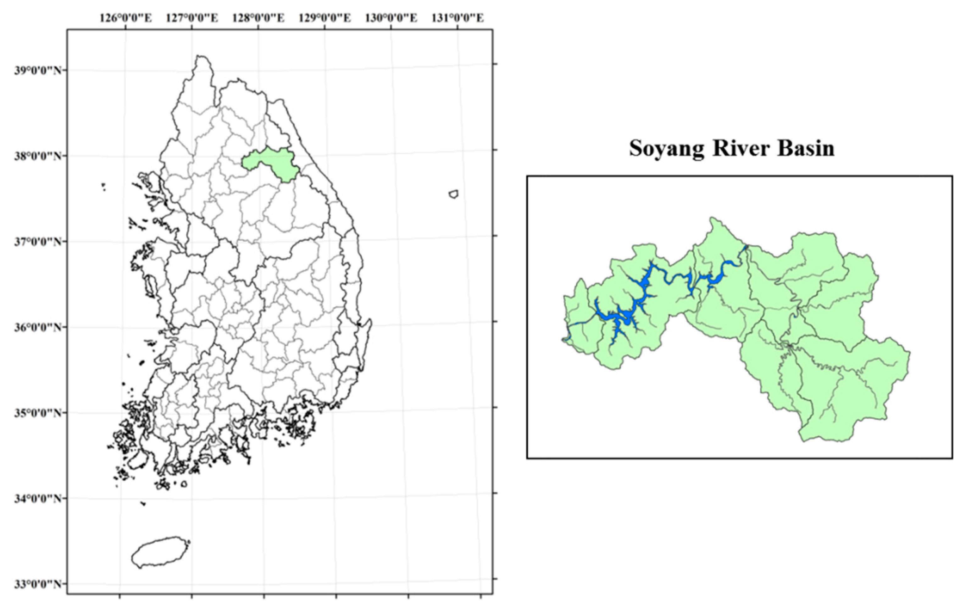
The target area is the Soyang River basin in South Korea described in Figure 1. It is one of the mid-sized basins located in the upper stream of Han River. Past observed daily streamflow data of the Soyang River basin were collected during 1976–2005, and future daily streamflow data were simulated according to precipitation estimates from the climate change scenarios for the period of 2011–2099 using the Precipitation Runoff Modeling System (PRMS). The PRMS was developed by United States Geological Survey for use in runoff analysis [21]. The 26 climate change scenarios using different Global Climate Models (GCMs) following RCP 8.5 were applied in this study and their details are depicted in

Table 1. Information of climate change scenarios.

No.	GCMs	Resolution	Institution
1	BCC-CSM1-1	2.813 × 2.791	Beijing Climate Center, China Meteorological Administration
2	BCC-CSM1-1-M	1.125 × 1.122
3	CanESM2	2.813 × 2.791	Canadian Centre for Climate Modelling and Analysis
4	CCSM4	1.250 × 0.942	Centro Euro-Mediterraneo per I Cambiamenti Climatici
5	CESM1-BGC	1.250 × 0.942	National Center for Atmospheric Research
6	CESM1-CAM5	1.250 × 0.942
7	CMCC-CM	0.750 × 0.748	Centro Euro-Mediterraneo per I Cambiamenti Climatici
8	CMCC-CMS	1.875 × 1.865
9	CNRM-CM5	1.406 × 1.401	Centre National de Recherches Meteorologiques
10	FGOALS-s2	2.813 × 1.659	LASG, Institute of Atmospheric Physics, Chinese Academy of Sciences
11	GFDL-ESM2G	2.500 × 2.023	Geophysical Fluid Dynamics Laboratory
12	GFDL-ESM2M	2.500 × 2.023
13	HadGEM2-AO	1.875 × 1.250	Met Office Hadley Centre
14	HadGEM2-CC	1.875 × 1.250
15	HadGEM2-ES	1.875 × 1.250
16	INM-CM4	2.000 × 1.500	Institute for Numerical Mathematics
17	IPSL-CM5A-LR	3.750 × 1.895	Institut Pierre-Simon Laplace
18	IPSL-CM5A-MR	2.500 × 1.268
19	IPSL-CM5B-LR	3.750 × 1.895
20	MIROC5	1.406 × 1.401	Atmosphere and Ocean Research Institute (The University of Tokyo)
21	MIROC-ESM	2.813 × 2.791	Japan Agency for Marine-Earth Science and Technology, Atmosphere and Ocean Research Institute (The University of Tokyo), and National Institute for Environmental Studies
22	MIROC-ESM-CHEM	2.813 × 2.791
23	MPI-ESM-LR	1.875 × 1.865	Max Planck Institute for Meteorology (MPI-M)
24	MPI-ESM-MR	1.875 × 1.865
25	MRI-CGCM3	1.125 × 1.122	Meteorological Research Institute
26	NorESM1-M	2.500 × 1.895	Norwegian Climate Centre

. The statistical downscaling of GCMs was performed by Eum and Cannon [22].

3. Methodology

3.1. Definition of Low-Flow Event and Water Supply Performance Indices

A flow duration curve (FDC) that shows the percent of times that a given discharge is exceeded, or equaled, is widely applied for the threshold level of the streamflow drought definition [23,24,25,26]. In this study, the 80th percentile of FDC was chosen as the threshold using past streamflow data. Low streamflow provoked by the deficit of precipitation may cause a water supply failure.

The future period (2011–2099) was divided into 85 blocks using a 5-year moving window (MV), i.e., MV1 (2011–2015), MV2 (2012–2016), and so on. The characteristics of low-flow events were defined in each moving window as reliability (rel) and vulnerability (vul), as proposed by Hashimoto et al. [27] to describe the performance of water resource systems under drought conditions.

Reliability is originally defined as the probability that the desired water demand is fully supplied to users within the design period. However, in this study, reliability was expressed as Equation (1), which is the ratio of the failure period and the total design period. Vulnerability refers to the quantitative risk of water supply failure, that is, the potential magnitude or damage of failure events. Vulnerability can be estimated as the mean of the total deficit during failures as shown in Equation (2).

$$rel={\displaystyle {\sum }_{n=1}^N{d}_n}/T,$$

(1)

$$vul={\displaystyle {\sum }_{n=1}^N{s}_n}/N,$$

(2)

where T is the total design period and N is the number of event occurrences during design period. In this study, T is 1825 days because a 5-year moving window was used for the design period. $d_n$ is the duration and $s_n$ is the total deficit or magnitude of the nth low-flow event.

3.2. Time-Varying Copula Model Using GAMLSS

The nonstationary analysis may be modeled assuming the parameters are time-dependent. The mean and standard deviation are generally employed for time-varying modeling, however, shape parameters are usually considered to be constant coefficients. Rigby and Stasinopoulos [10] proposed GAMLSS that can involve two to four parameters, i.e., location (mean), scale (standard deviation), and shape (skewness, kurtosis) parameters.

A GAMLSS assumes independent observations $y_i$ for $i=1,2$ ($y_1=\left\{re{l}_1,re{l}_2,\cdots ,re{l}_p\right\}$ and $y_2=\left\{vu{l}_1,vu{l}_2,\cdots ,vu{l}_p\right\}$) with probability function $f(y_i|{\mathsf{\Theta }}_i)$. ${\mathsf{\Theta }}_i=\left({\mu }_i,{\sigma }_i\right)$ is a vector of distribution parameters, which are ${\mu }_i=\left\{{\mu }_1,{\mu }_2,\cdots ,{\mu }_p\right\}$ and ${\sigma }_i=\left\{{\sigma }_1,{\sigma }_2,\cdots ,{\sigma }_p\right\}$. Each parameter can be related to explanatory variables. Since we assumed the drought risk to be time-dependent and induced by climate change, time was selected as an explanatory variable in the study. Explanatory variable $t_k$, $g(\cdot )$ is a known link function relating $\mathsf{\Theta }$ to $t_k$ given by Equation (3) without an additive term of random effects.

$$g_k({\theta }_k)={\eta }_k=\mathsf{\beta }{t}_k,$$

(3)

where $\mathsf{\beta }$ is the vector of estimated coefficient of time-varying parameters and the length of $\mathsf{\beta }$ can be two or four, described as Equation (5). The explanatory variable time $t_k=\left\{t_1,t_2,\cdots ,t_p\right\}=\left\{1,2,\cdots ,p\right\}$ is the number of the moving window, thus p is the length of the datasets (reliability and vulnerability).

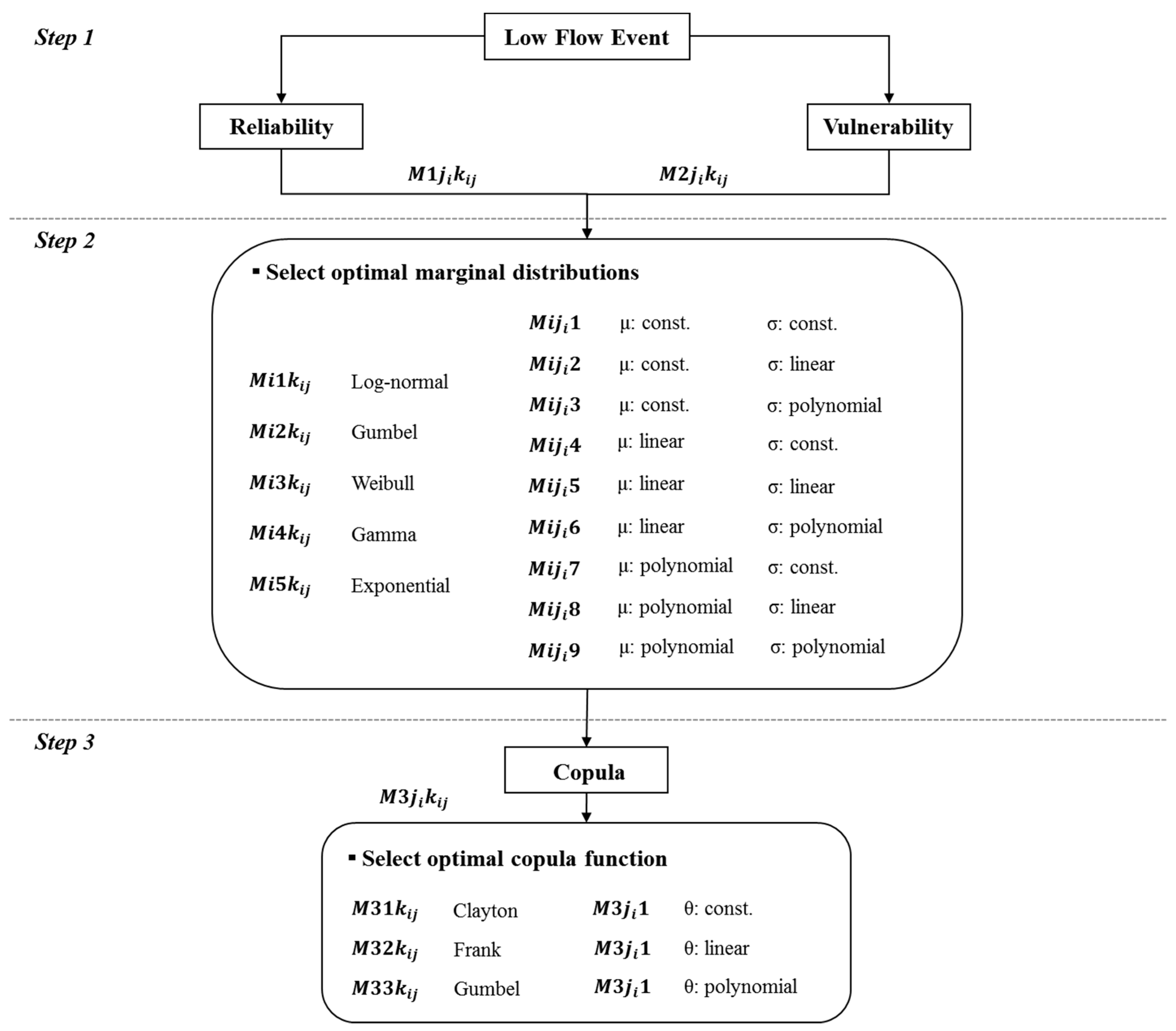
The joint cumulative distribution function (JCDF) is expressed using copula of two random variables of reliability and vulnerability, as shown in Equation (4). The implementation of the time-varying copula model includes three major steps, as shown in Figure 2: (1) The estimation of reliability and vulnerability, (2) the estimation of the marginal distribution, and (3) the modeling of the copula parameter depending on the margins.

The parameters of marginal distributions (${\mathsf{\Theta }}_i$) and copula ($\theta$) were assumed to be constant, linear, or polynomial function as Equation (5). The parametric vector ${\beta }_k$ were estimated within the GAMLSS framework by maximizing the log–likelihood function for copula with continuous margins written as Equation (6) [28].

$$F(y_1,y_2|\vartheta )=C\left(F_1(y_1|{\mu }_1,{\sigma }_1),F_2(y_2|{\mu }_2,{\sigma }_2);\theta \right),$$

(4)

$${\eta }_k=const.,$$

(5a)

$${\eta }_k={\beta }_0+{\beta }_{1}t,$$

(5b)

$${\eta }_k={\beta }_0+{\beta }_{1}t+{\beta }_2{t}^2+{\beta }_3{t}^3,$$

(5c)

$$\log L(\vartheta )={\displaystyle \sum _{k=1}^p\log \left\{c(F_1(y_{1k}|{\mu }_{1k},{\sigma }_{1k}),F_2(y_{2k}|{\mu }_{2k},{\sigma }_{2k});{\theta }_k\right\}}+{\displaystyle \sum _{k=1}^p{\displaystyle \sum _{i=1}^2\log \left\{f_i(y_{ik}|{\mu }_{ik},{\sigma }_{ik})\right\}}}$$

(6)

where C and c are joint cumulative distribution function and joint probability density function estimated by copula, respectively. $\vartheta =\left\{{\mathsf{\Theta }}_1,{\mathsf{\Theta }}_2,\theta \right\}$ is a set of distribution parameters used in a time-dependent copula model.

3.3. Joint Drought Management Index (JDMI)

From Equation (4), the JCDF with bivariate marginal, $u=F_1(y_1|{\mathsf{\Theta }}_1)$ and $v=F_2(y_2|{\mathsf{\Theta }}_2)$ is expressed as shown in Equation (7). The cumulative probability q is usually treated as an indicator of a destructive event, thus a smaller q implies a less-dry condition. Therefore, it would be of interest in the risk analysis to know what the probability is for a random event. In this context, Salvadori and De Michele [29] adopted Kendall distribution of Archimedean copulas.

A Kendall distribution is useful to project multivariate information onto a single dimension as described as Equation (8). The copula function can have the same quantiles with different combinations of variables, e.g., C(u,v) = q and C(u*,v*) = q. Therefore, it is difficult to specify the drought characteristics with the copula quantile. Since the JDMI implied the joint probability of nonexceedance of water supply performance indices, it is important to capture the ranges of sets of variables that can produce the same quantile.

In this study, the JDMI was designed to increase when reliability and vulnerability increase and vice versa. In other words, the larger the JDMI, the higher the risk. From the probability of Kendall distribution shown in Equation (8), the JDMI can be defined as shown in Equation (9).

$$C(u,v)=P\left[Y_1\le rel*,Y_2\le vul*\right]=C\left[F_1(Y_1|{\mathsf{\Theta }}_1),F(Y_2|{\mathsf{\Theta }}_2)\right]=q,$$

(7)

$$K_c(q)=P\left[C(u,v)\le q\right],$$

(8)

$$JDMI={\varphi }^{-1}\left(K_c(q)\right),$$

(9)

where rel* and vul* are random values of reliability and vulnerability, respectively. $\varphi$ is the standard normal distribution function.

4. Results and Discussion

4.1. Drought Events and Water Supply Performance Indices

The drought was defined as a period in which flow is equal or less than Q80 calculated from observed data, so that future drought risk could be assessed and compared with the past. Water supply performance indices were estimated based on low-flow drought events. The Mann–Kendall (MK) test was employed to find the monotonic trend in reliability and vulnerability estimated in 85 moving windows.

The monotonic trend was observed in 15 scenarios for reliability and vulnerability, but the scenarios were not identical. The Z-statistics of the MK test suggested that there was a significant decreasing trend in reliability in the 20 scenarios with the significance level of 0.05. A decreasing trend for vulnerability that was observed in 16 scenarios, while a significant increasing trend was observed in 10 scenarios. Thus, it is expected that the duration and the magnitude of future hydrological droughts would be less than those of the past.

The multi-index using water supply performance indices have already been tested in previous research. The drought management index (DMI) was developed using resilience and vulnerability, that account for the ability of the system to recover from drought damage [30,31]. On the contrary, the JDMI inspired by the DMI is estimated based on D and S. Thus, the JDMI can reflect the drought aspects that cause damage to the system.

4.2. Model Selection and Parameter Estimation

Five probability distributions in

Table 2. Definition and properties of the marginal distributions used in the study.

Distribution	PDF	Link Function
	${\mathit{f}}_{\mathit{m}}({\mathit{y}}_{\mathit{m}}|{\mathit{\mu }}_{\mathit{m}},{\mathit{\sigma }}_{\mathit{m}})$	${\mathit{g}}_{\mathit{m}}({\mathit{\mu }}_{\mathit{m}})$	${\mathit{g}}_{\mathit{m}}({\mathit{\sigma }}_{\mathit{m}})$
Log-normal	$\frac{1}{y\sigma \sqrt{2\pi }}\exp \left[-\frac{{\left\{\log (y)-\mu \right\}}^2}{2{\sigma }^2}\right]$	$\log ({\mu }_m)$	$\log ({\sigma }_m)$
Gumbel	$\frac{1}{\sigma }\exp \left\{\left(\frac{y-\mu }{\sigma }\right)-\exp \left(\frac{y-\mu }{\sigma }\right)\right\}$	${\mu }_m$	$\log ({\sigma }_m)$
Weibull	$\frac{\sigma }{\mu }{\left(\frac{y}{\mu }\right)}^{\sigma -1}\exp \left\{-{\left(\frac{y}{\mu }\right)}^{\sigma }\right\}$	$\log ({\mu }_m)$	$\log ({\sigma }_m)$
Gamma	$\frac{1}{{(\mu {\sigma }^2)}^{1/{\sigma }^2}}\frac{y^{1/{\sigma }^2-1}\exp \left(-y/\mu {\sigma }^2\right)}{\mathsf{\Gamma }\left(1/{\sigma }^2\right)}$	$\log ({\mu }_m)$	$\log ({\sigma }_m)$
Exponential	$\frac{1}{\mu }{\mathrm{e}}^{-\raisebox{1ex}{$y$}\!\left/ \!\raisebox{-1ex}{$\mu $}\right.}$	$\log ({\mu }_m)$	—

, i.e., log-normal, Gumbel, Weibull, Gamma, and exponential distribution, were explored to define the appropriate marginal distributions of reliability and vulnerability. In addition to investigating the relationship between the two margins, three copula functions in

Table 3. Definition and properties of the Archimedean copula used in the study ($\mathbf{\epsilon }={\mathbf{10}}^{-7}$).

Copula	CDF	Link Function
	$\mathit{C}(\mathbf{u},\mathbf{v};\mathit{\theta })$	$\mathit{g}(\mathit{\theta })$
Clayton	${\left(u^{-\theta }+v^{-\theta }-1\right)}^{-\raisebox{1ex}{$1$}\!\left/ \!\raisebox{-1ex}{$\theta $}\right.}$	$\log (\theta -\epsilon )$
Frank	$-\frac{1}{\theta }\log \left\{\frac{1+(e^{-\theta u}-1)(e^{-\theta v}-1)}{e^{-\theta }-1}\right\}$	$\theta$
Gumbel	$\exp \left[-{\left\{{(-\log u)}^{\theta }+{(-\log v)}^{\theta }\right\}}^{\raisebox{1ex}{$1$}\!\left/ \!\raisebox{-1ex}{$\theta $}\right.}\right]$	$\log (\theta -1-\epsilon )$

, i.e., Clayton, Frank, and Gumbel copula, were tested. The parameters of marginal distributions and copula were assumed to be a function of the explanatory variable, which is time, t.

The time-dependent copula model was fitted by the nonstationary marginal distributions. The parameters of the margins and copula were assumed to be constant, linear, and polynomial functions with the design parameters and time as described in Equations 5a, 5b, and 5c, respectively. If the parameters are independent from time, the model will be stationary with constant parameters.

Table 4. Time-dependent copula model selection of each scenarios.

SCN	Reliability			Vulnerability			Copula
	Distribution		P-KS	Distribution	P-KS		Distribution	AIC
S#01	Weibull	M134	0.31	Weibull	M231	0.91	Clayton	M313	455.21
S#02	Weibull	M132	0.48	log-normal	M215	0.09	Gumbel	M333	430.79
S#03	Weibull	M131	0.93	Weibull	M235	0.62	Frank	M323	428.96
S#04	Gamma	M141	0.76	log-normal	M211	1.00	Gumbel	M333	443.54
S#05	Weibull	M137	0.67	log-normal	M213	0.20	Gumbel	M333	444.26
S#06	log-normal	M113	0.97	log-normal	M211	0.73	Clayton	M313	414.55
S#07	Weibull	M134	0.51	log-normal	M214	0.33	Gumbel	M333	413.12
S#08	Gamma	M144	0.46	log-normal	M214	0.18	Clayton	M313	472.41
S#09	Weibull	M131	0.86	log-normal	M211	0.98	Gumbel	M333	415.80
S#10	Gamma	M147	0.33	log-normal	M212	0.68	Clayton	M313	443.71
S#11	Weibull	M131	0.67	Gamma	M241	0.80	Frank	M323	446.45
S#12	Weibull	M135	0.11	log-normal	M214	0.34	Gumbel	M333	419.45
S#13	Weibull	M131	0.54	log-normal	M212	0.60	Gumbel	M333	439.64
S#14	Gamma	M142	0.10	Gamma	M247	0.22	Clayton	M313	405.54
S#15	Weibull	M138	0.75	Gamma	M241	0.26	Clayton	M313	417.80
S#16	Gamma	M145	0.28	log-normal	M213	0.35	Gumbel	M333	419.98
S#17	Weibull	M135	0.56	Gamma	M247	0.75	Clayton	M313	429.78
S#18	Weibull	M137	0.92	Gamma	M241	1.00	Frank	M323	420.80
S#19	Weibull	M134	0.63	log-normal	M211	0.34	Frank	M323	447.95
S#20	log-normal	M111	0.76	Gamma	M247	0.07	Clayton	M313	399.52
S#21	log-normal	M113	0.54	Gumbel	M224	0.42	Clayton	M313	443.96
S#22	Weibull	M133	0.88	Weibull	M232	0.95	Frank	M323	412.28
S#23	log-normal	M111	0.90	Gamma	M241	0.39	Frank	M323	419.94
S#24	Gamma	M144	0.60	log-normal	M211	0.49	Gumbel	M333	415.35
S#25	Gamma	M145	0.08	log-normal	M214	0.64	Gumbel	M333	397.11
S#26	Gamma	M145	0.27	Gamma	M243	0.23	Gumbel	M333	446.31

* P-KS is the p-value of the Kolmogorov–Smirnov (KS) test; if the p-value is larger than a significance level (0.05), the result of distribution selection is valid.

represents the result of model selection. It was decided that the distributions of best fit for reliability and vulnerability were the Weibull and log-normal, respectively. The p-value of the Kolmogorov–Smirnov (KS) test for each marginal distribution supported the model decision with 5% significance level. Finally, the most appropriate copula models were determined based on the Akaike information criterion (AIC), and Gumbel was dominantly selected.

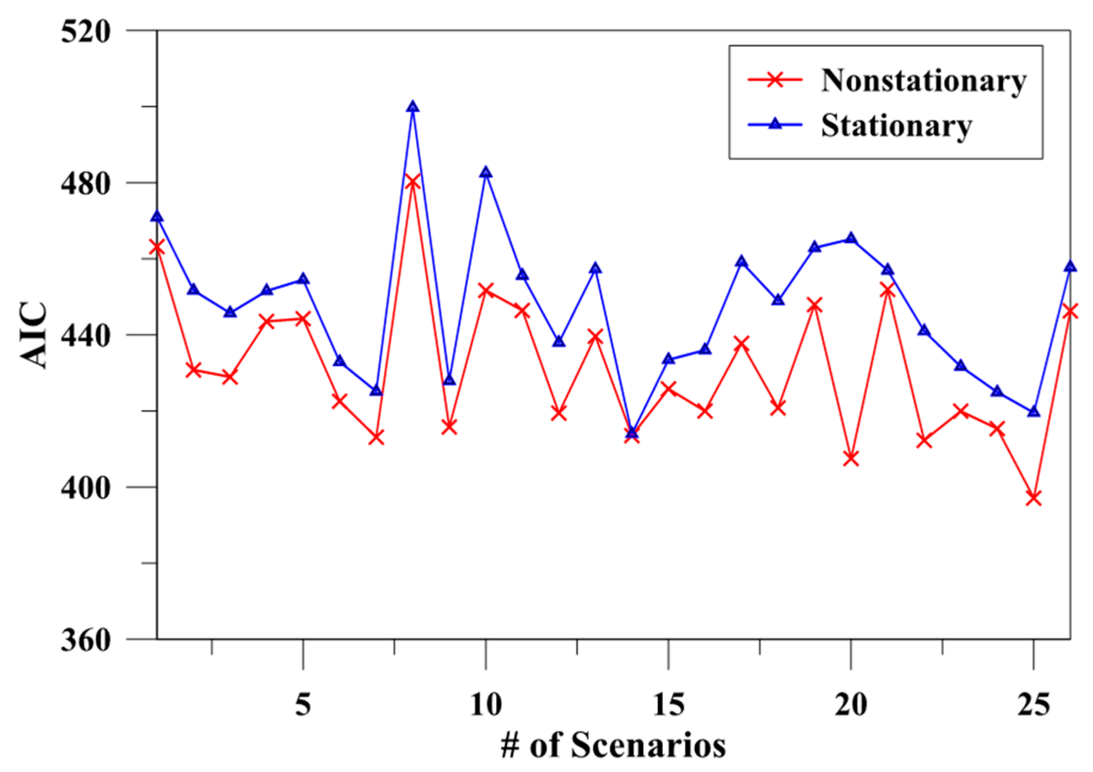
The stationary copula models were also estimated for comparison. Figure 3 describes the AIC comparison between the stationary and nonstationary copula models. The AIC values of nonstationary models were estimated to be lower than those of stationary models in all scenarios. The lower AIC indicates a better model, thus, the time-dependent copula would be more appropriate in the study area. It should be noted that the marginal distributions and the copula of the stationary and nonstationary model were not identical; log-normal was selected for all of the margins and Gumbel copula was dominant for the stationary model.

4.3. Risk Assessment Based on Nonstationary JDMI

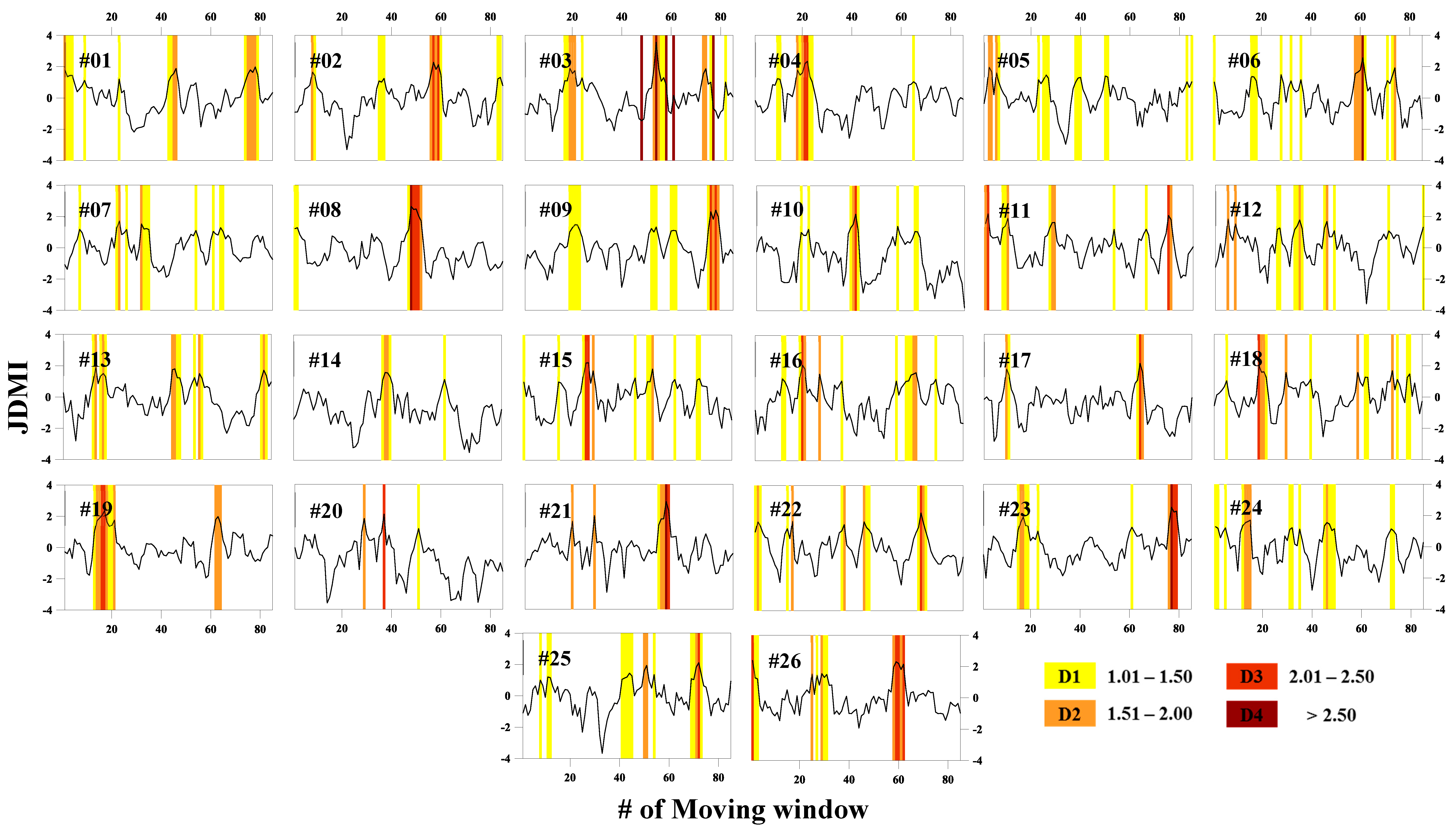
The drought event was defined when both reliability and vulnerability were larger than average values in a probabilistic approach. The droughts based on JDMI can be classified into five states, i.e., normal (D0), mild (D1), moderate (D2), severe (D3), and extreme (D4). Figure 4 shows the drought state classification based on the JDMI estimated for all scenarios.

The future period was divided into three time domains to clarify drought occurrence patterns and their characteristics. The periods of P1 (2011–2040), P2 (2041–2070), and P3 (2071–2099) can be substituted to the moving windows, which are MV1–30, MV31–60, and MV61–85, respectively. In other words, each period consists of about 30 different 5-year moving windows: (1) P1: MV1 (2011–2015) to MV30 (2040–2044); (2) P2: MV31 (2041–2045) to MV60 (2070–2074); (3) P3: MV61 (2071–2075) to MV85 (2095–2099).

As shown in Figure 4, the extreme drought (D4) rarely occurred but only five events were observed in all scenarios (scenario #03, #6, #08, #21, and #23), and appeared in P2 and P3. The number of droughts was larger in P1 compared with P2 and P3, however, the mild and moderate droughts (D1 and D2) were concentrated in P1. Among the scenarios, results from the severe and extreme drought (D3 and D4) occurrences were slightly more frequent in P2 and P3 than P1. Nevertheless, it was obvious that drought appearance declined in P2 and P3; thus, P1 would be more prone to water deficit.

Table 5. Maximum events based on JDMI of each scenario and the corresponding values of reliability and vulnerability.

SCN	# of Moving Window (year)		JDMI	Reliability	Vulnerability (m3/s)
S#01	78	(2088–2092)	1.98	0.46	570.15
S#02	57	(2067–2071)	2.28	0.39	929.20
S#03	54	(2064–2068)	3.56	0.32	780.31
S#04	22	(2032–2036)	2.36	0.40	1078.86
S#05	3	(2013–2017)	1.98	0.33	550.76
S#06	61	(2071–2075)	2.56	0.31	926.85
S#07	23	(2033–2037)	1.73	0.34	563.84
S#08	48	(2058–2062)	2.64	0.43	1273.97
S#09	78	(2088–2092)	2.40	0.42	783.54
S#10	41	(2051–2055)	2.18	0.50	892.56
S#11	2	(2012–2016)	2.19	0.39	838.17
S#12	6	(2016–2020)	1.86	0.25	781.09
S#13	14	(2024–2028)	1.93	0.34	749.63
S#14	38	(2048–2052)	1.62	0.35	792.17
S#15	27	(2037–2041)	2.26	0.33	685.77
S#16	20	(2030–2034)	2.14	0.31	778.84
S#17	64	(2074–2078)	2.15	0.40	816.04
S#18	19	(2029–2033)	2.03	0.36	743.18
S#19	17	(2027–2031)	2.39	0.35	814.58
S#20	37	(2047–2051)	2.09	0.37	992.74
S#21	58	(2068–2072)	2.89	0.37	1075.18
S#22	68	(2078–2082)	2.25	0.33	908.85
S#23	77	(2087–2091)	2.53	0.36	704.78
S#24	15	(2025–2029)	1.73	0.21	545.02
S#25	72	(2082–2086)	2.12	0.29	497.73
S#26	1	(2011–2015)	2.39	0.36	633.40

depicts the maximum drought events in all scenarios and the corresponding values of reliability and vulnerability. Reliability and vulnerability could be representative of drought duration and magnitude and, thus, we can deduce the drought characteristics from those indexes. In the S#01, for example, reliability and vulnerability were estimated as 0.46 and 570.15 m³/s based on JDMI of 1.98. During a 5-year moving window, the expected drought occurrence duration would be 0.46 × 365 (days) × 5 (years) = 839.5 days. Also, the expected maximum drought magnitude would be 570.15 × 24 (h) × 60 (min) × 60 (s) = 49,260,960 m³ per day, due to the daily streamflow data basis.

The JDMI can quantify the potential hydrological drought characteristics that would cause severe water shortage every five years. According to Table 5, the corresponding values of reliability and vulnerability of each maximum JDMI ranged from 0.21 to 0.50, and from 497.73 to 1273.97 m³/s, respectively. Therefore, it is expected for the Soyang River basin that the maximum drought damage would last at least 386 to 915 days and induce a water deficit from 43 × 10⁶ to maximum 110 × 10⁶ m³ for an event during five years (represented as 5-year moving window in the study).

5. Summaries and Conclusions

This study proposed the nonstationary JDMI built under the time-dependent copula model to assess the potential risk of hydrological droughts that could induce water deficit. The focus was on the nonstationarity in the parameters of distribution function of margins and copula detected using the GAMLSS framework. The appropriate model selection procedure was generally carried out based on the log–likelihood functions and AIC.

The data corresponding to 26 climate change scenarios of Soyang River basin of were used in the analysis. The future low-flow drought was defined using the future simulated data, but the threshold level was estimated from past data. The water supply performance indexes, reliability and vulnerability, were respectively calculated from the duration and magnitude of the drought events occurring in 5-year moving windows.

Not all marginal distributions were found to be nonstationary based on the MK test, however, some of the datasets showed best fitting when using the time-varying parameter, even when they were under a stationary condition. It should be noted that among 11 datasets of reliability and vulnerability revealed not to have a trend, the constant parameters showed the best fitting for only 5 and 6 datasets, respectively. On the other hand, the copula with the polynomial function of time for the dependence parameter had better performance than the one with the constant or linear functions in all datasets. Therefore, we can conclude that the time-varying model is more suitable for the study area.

An appropriate drought index can serve as the important base in drought management, preparation, and mitigation. The nonstationary JDMI may provide the expected quantities of drought risk under changing environmental conditions. Therefore, it is possible to establish the targeted safety level through reliability and vulnerability, which are corresponding values of JDMI in the specific period. Water supply safety assessment is a priority for drought response/mitigation and also water supply system design.

However, the nonstationary model developed in this research does not include other hydrometeorological variables, with only time as an explanatory variable. Thus, it cannot fully consider the nonstationary behaviors of drought characteristics. However, the multi-index would increase uncertainty by combining the variables in a probabilistic approach. Nevertheless, future studies should establish new drought indexes with climate variables, i.e., temperature, precipitation, and evaporation.

References

- Milly, P.C.D.; Betancourt, J.; Falkenmark, M.; Hirsch, R.M.; Kundzewicz, Z.W.; Lettenmaier, D.P.; Stouffer, R.J. Stationarity is Dead: Whither Water Management? Science 2008, 319, 573–574. [Google Scholar] [CrossRef]
- Kendall, M.G. Rank correlation methods. Biometrika 1957, 44, 298. [Google Scholar] [CrossRef]
- Mann, H.B. Nonparametric Tests Against Trend. Econometrica 1945, 13, 245–259. [Google Scholar] [CrossRef]
- Pettitt, A.N. A Non-Parametric Approach to the Change-Point Problem. Appl. Stat. 1979, 28, 126–135. [Google Scholar] [CrossRef]
- Strupczewski, W.G.; Singh, V.P.; Feluch, W. Non-stationary approach to at-site flood frequency modelling I. Maximum likelihood estimation. J. Hydrol. 2001, 248, 123–142. [Google Scholar] [CrossRef]
- El Adlouni, S.; Ouarda, T.B.M.J.; Zhang, X.; Roy, R.; Bobée, B. Generalized maximum likelihood estimators for the nonstationary generalized extreme value model. Water Resour. Res. 2007, 43. [Google Scholar] [CrossRef] [Green Version]
- Read, L.K.; Vogel, R.M. Reliability, return periods, and risk under nonstationarity. Water Resour. Res. 2015, 51, 6381–6398. [Google Scholar] [CrossRef] [Green Version]
- Sugahara, S.; da Rocha, R.P.; Silveira, R. Non-stationary frequency analysis of extreme daily rainfall in Sao Paulo, Brazil. Int. J. Climatol. 2009, 29, 1339–1349. [Google Scholar] [CrossRef] [Green Version]
- Wi, S.; Valdés, J.B.; Steinschneider, S.; Kim, T.W. Non-stationary frequency analysis of extreme precipitation in South Korea using peaks-over-threshold and annual maxima. Stoch. Environ. Res. Risk Assess. 2015, 30, 583–606. [Google Scholar] [CrossRef]
- Rigby, R.A.; Stasinopoulos, D.M. Generalized additive models for location, scale and shape. J. R. Stat. Soc. Ser. C-Appl. Stat. 2005, 54, 507–544. [Google Scholar] [CrossRef]
- Du, T.; Xiong, L.; Xu, C.Y.; Gippel, C.J.; Guo, S.; Liu, P. Return period and risk analysis of nonstationary low-flow series under climate change. J. Hydrol. 2015, 527, 234–250. [Google Scholar] [CrossRef]
- Yan, L.; Xiong, L.; Guo, S.; Xu, C.-Y.; Xia, J.; Du, T. Comparison of four nonstationary hydrologic design methods for changing environment. J. Hydrol. 2017, 551, 132–150. [Google Scholar] [CrossRef]
- Ahn, K.H.; Palmer, R.N. Use of a nonstationary copula to predict future bivariate low flow frequency in the Connecticut river basin. Hydrol. Process. 2016, 30, 3518–3532. [Google Scholar] [CrossRef]
- Jiang, C.; Xiong, L.; Wang, D.; Liu, P.; Guo, S.; Xu, C.Y. Separating the impacts of climate change and human activities on runoff using the Budyko-type equations with time-varying parameters. J. Hydrol. 2015, 522, 326–338. [Google Scholar] [CrossRef]
- Zhang, T.; Wang, Y.; Wang, B.; Tan, S.; Feng, P. Nonstationary Flood Frequency Analysis Using Univariate and Bivariate Time-Varying Models Based on GAMLSS. Water 2018, 10, 819. [Google Scholar] [CrossRef]
- Wang, Y.; Li, J.; Feng, P.; Hu, R. A Time-Dependent Drought Index for Non-Stationary Precipitation Series. Water Resour. Manag. 2015, 29, 5631–5647. [Google Scholar] [CrossRef]
- Bazrafshan, J.; Hejabi, S. A Non-Stationary Reconnaissance Drought Index (NRDI) for Drought Monitoring in a Changing Climate. Water Resour. Manag. 2018, 32, 2611–2624. [Google Scholar] [CrossRef]
- Intergovernmental Panel on Climate Change. Climate Change 2014 Mitigation of Climate Change; Cambridge University Press: Cambridge, UK, 2014. [Google Scholar] [CrossRef]
- Suh, M.S.; Oh, S.G.; Lee, Y.S.; Ahn, J.B.; Cha, D.H.; Lee, D.K.; Hong, S.Y.; Min, S.K.; Park, S.C.; Kang, H.S. Projections of high resolution climate changes for South Korea using multiple-regional climate models based on four RCP scenarios. Part 1: Surface air temperature. Asia-Pac. J. Atmos. Sci. 2016, 52, 151–169. [Google Scholar] [CrossRef]
- Oh, S.G.; Suh, M.S.; Lee, Y.S.; Ahn, J.B.; Cha, D.H.; Lee, D.K.; Hong, S.Y.; Min, S.K.; Park, S.C.; Kang, H.S. Projections of high resolution climate changes for South Korea using multiple-regional climate models based on four RCP scenarios. Part 2: Precipitation. Asia-Pac. J. Atmos. Sci. 2016, 52, 171–189. [Google Scholar] [CrossRef]
- Markstrom, S.L.; Regan, R.S.; Hay, L.E.; Viger, R.J.; Webb, R.M.; Payn, R.A.; LaFontaine, J.H. PRMS-IV, the precipitation-runoff modeling system, version 4. US Geol. Surv. Tech. Methods 2015, 6-B7. [Google Scholar] [CrossRef]
- Eum, H.I.; Cannon, A.J. Intercomparison of projected changes in climate extremes for South Korea: Application of trend preserving statistical downscaling methods to the CMIP5 ensemble. Int. J. Climatol. 2017, 37, 3381–3397. [Google Scholar] [CrossRef]
- Beyene, B.S.; Van Loon, A.F.; Van Lanen, H.A.J.; Torfs, P.J.J.F. Investigation of variable threshold level approaches for hydrological drought identification. Hydrol. Earth Syst. Sci. Discuss. 2014, 11, 12765–12797. [Google Scholar] [CrossRef]
- Fleig, A.K.; Tallaksen, L.M.; Hisdal, H.; Demuth, S. A global evaluation of streamflow drought characteristics. Hydrol. Earth Syst. Sci. 2006, 10, 535–552. [Google Scholar] [CrossRef] [Green Version]
- Rivera, J.A.; Araneo, D.C.; Penalba, O.C. Threshold level approach for streamflow drought analysis in the Central Andes of Argentina: A climatological assessment. Hydrol. Sci. J. 2017, 62, 1949–1964. [Google Scholar] [CrossRef]
- Tallaksen, L.M.; Madsen, H.; Clausen, B. On the definition and modelling of streamflow drought duration and deficit volume. Hydrol. Sci. J.-J. Des. Sci. Hydrol. 1997, 42, 15–33. [Google Scholar] [CrossRef] [Green Version]
- Hashimoto, T.; Stedinger, J.R.; Loucks, D.P. Reliability, Resiliency, and Vulnerability Criteria for Water-Resource System Performance Evaluation. Water Resour. Res. 1982, 18, 14–20. [Google Scholar] [CrossRef]
- Marra, G.; Radice, R. Bivariate copula additive models for location, scale and shape. Comput. Stat. Data Anal. 2017, 112, 99–113. [Google Scholar] [CrossRef] [Green Version]
- Salvadori, G.; De Michele, C. Frequency analysis via copulas: Theoretical aspects and applications to hydrological events. Water Resour. Res. 2004, 40, W12511. [Google Scholar] [CrossRef]
- Chanda, K.; Maity, R.; Sharma, A.; Mehrotra, R. Spatiotemporal variation of long-term drought propensity through reliability-resilience-vulnerability based Drought Management Index. Water Resour. Res. 2014, 50, 7662–7676. [Google Scholar] [CrossRef] [Green Version]
- Maity, R.; Sharma, A.; Nagesh Kumar, D.; Chanda, K. Characterizing Drought Using the Reliability-Resilience-Vulnerability Concept. J. Hydrol. Eng. 2013, 18, 859–869. [Google Scholar] [CrossRef]
Figure 1.
Study area.
Figure 2.
The time-dependent copula modeling procedure and model description.
Figure 3.
Akaike information criterion (AIC) comparison of nonstationary and stationary copula model.
Figure 4.
Joint drought management index (JDMI) estimation and drought state classification of 26 scenarios.