Remediation of Stormwater Pollutants by Porous Asphalt Pavement


1
Washington Stormwater Center, Washington State University, Puyallup, WA 98371, USA
2
Department of Crop, Soil and Environmental Sciences, Auburn University, Auburn, AL 35412, USA
3
Washington Stormwater Center, Washington State University, Puyallup, WA 98371, USA
4
Herrera Environmental Inc., Bellingham, WA 98225, USA
*
Author to whom correspondence should be addressed.
†
Current address: 2606 W Pioneer, Puyallup, WA 98371, USA.
Water 2019, 11(3), 520; https://doi.org/10.3390/w11030520
Submission received: 9 December 2018
/
Revised: 5 March 2019
/
Accepted: 6 March 2019
/
Published: 13 March 2019
(This article belongs to the Section Urban Water Management)
Abstract
:Porous Asphalt (PA) pavements are an increasingly adopted tool in the green stormwater infrastructure toolbox to manage stormwater in urbanized watersheds across the United States. This technology has seen particular interest in western Washington State, where permeable pavements are recognized as an approved best management practice per the National Pollutant Discharge Elimination System (NPDES) municipal stormwater permit. Stormwater effluent concentrations from six PA cells were compared with runoff concentrations from three standard impervious asphalt cells to quantify pollutant removal efficiencies by porous asphalt systems. Additionally, the effects of maintenance and pavement age on pollutant removal efficiencies were examined. Twelve natural and artificial storms were examined over a five-year period. Street dirt and pollutant spikes were added to the pavements prior to some storm events to simulate high loading conditions. Results from this work show that porous asphalt pavements are highly efficient at removing particulate pollutants, specifically coarse sediments (98.7%), total Pb ( 98.4%), total Zn (97.8%), and total suspended solids (93.4%). Dissolved metals and Polycyclic Aromatic Hydrocarbons (PAH) were not significantly removed. Removal efficiencies for total Pb, total Zn, motor oil, and diesel H. improved with the age of the system. Annual maintenance of the pavements with a regenerative air street sweeper did not yield significant pollutant removal efficiency differences between maintained and unmaintained PA cells.
1. Introduction
Stormwater pollution is a critical source of impairment to receiving water bodies in the United States. In western Washington State, stormwater is a principal threat to the Puget Sound ecosystem [1]. Green Stormwater Infrastructure (GSI) is a system of practices that aim to mitigate both water quantity and quality issues employing ecosystem processes to treat stormwater close to its source [2,3,4]. For a wider perspective on the advantages and appropriateness of GSI systems to manage stormwater, see Pataki et al. [5], Lucas and Sample [6], Pennino et al. [7], Miles and Band [8]. In western Washington State, GSI is a requirement of the National Pollutant Discharge Elimination System (NPDES) municipal stormwater permit for certain new and redevelopment projects [9].
An important tool in the GSI toolbox is permeable pavements, a system that sees widening adoption in municipalities across the United States [10,11]. Permeable pavements typically consist of a permeable upper wearing course supported by a layer of coarse aggregate material that also functions as a reservoir for stormwater infiltrating through the upper porous wearing course. Ultimately, the stormwater that is stored temporarily in the aggregate reservoir layer gradually exfiltrates into the native soils below [12,13]. Permeable pavements are typically not suited where native soils have very low infiltration rates; however, with an overflow drain in the reservoir layer, permeable pavements can be adapted for use in low infiltration soils.
Porous asphalt is a specific type of permeable pavement that incorporates hot-mix asphalt to form the upper wearing layer. Porous asphalt differs from standard hot-mix asphalt in that finer aggregates are precluded [14] from the mix. Roseen et al. [15] pointed out that the process of creating a porous asphalt mix has been in place for several decades in the form of Open-Graded Friction Course (OGFC), a process of installing a thin surface porous layer overlaying an impervious standard asphalt layer. The distinction between OGFC and porous asphalt is that the porous layer extends all the way to the supporting coarse aggregate layer below. Typical porous asphalt is currently only suitable for low traffic uses such as parking lots, sidewalks, and driveways [15,16,17]. However, recent incorporations of additional materials like carbon fiber and Kevlar strands to the asphalt are purported to improve the durability of the wearing course [16,18].
In a review of published studies that measured the effectiveness of Low Impact Development (LID) practices, Ahiablame et al. [19] reported that permeable pavements reduce runoff generation between 50 and 93% and may eliminate runoff completely in some cases, e.g., [15,20,21]. While this study aims to report the results of water quality mitigation by a system of porous asphalt pavement cells, a companion study on these same cells showed that porous asphalt cells are capable of infiltrating around 99% of incident rainfall into the coarse aggregate layer below [20].
1.1. Pollutant Removal by Permeable Pavements
Typical stormwater pollutants in urban runoff include a large suite of pollutants that range from particulate sediments to organic hydrocarbons in a dissolved phase. Most pollutants in urban stormwater are derived from wet and dry deposition of industrial, vehicular, and residential-sourced pollutants [22]. Malmqvist [23] showed that by identifying sources of pollutants in urban catchments, steps can be taken to limit nutrient and metal loadings to receiving waters. In a study of tropical urban catchments, Chow and Yusop [24] showed that most stormwater pollutants in residential areas came from lawns and gardens, and in industrial zones from factory and workshop lots. In a comprehensive study on urban stormwater samples from the Birmingham, AL, area, Pitt et al. [25] found that organic pollutants such as Polycyclic Aromatic Hydrocarbon (PAH) loadings were greatest from parking lots and areas where vehicles are serviced. This study also showed that of all areas and pollutants considered, storage areas and parking lots were the most toxic per a microbics-suggested toxicity protocol. Lee and Bang [26] analyzed pollutant loads from nine cities in Korea and showed that the highest nutrient loads per unit area came from high-density residential areas; metals and organic pollutants were not evaluated. However, a study of highway runoff by Du et al. [27] detected a large fraction of new organic contaminants, several that have yet to be fully characterized. Four mechanisms are broadly understood to impact pollutant fate within permeable pavements, and these are biological action [28], adsorption, filtration [29,30], and desorption [31]. For particulate pollutants like total suspended solids (TSS), filtration is thought to be the prevalent mechanism for removal [32].
In a study using simulated storm events on a series of permeable pavement blocks at a laboratory bench-top scale, Tota-Maharaj and Scholz [33] found that TSS removal efficiencies ranged from 53–94%. In addition, Tota-Maharaj and Scholz [33] showed that average nitrate-nitrogen removal efficiencies ranged between 41 and 63%, and ammonia-nitrogen removal efficiency was also reported to be over 70%, average orthophosphate-phosphorous around 78%, and a mean microbial removal efficiency of 98%. Brown et al. [34] reported TSS removal of around 80% for a TSS size fraction m with open jointed paving blocks and porous asphalt pavements. In a summary of studies related to pollutant removal by porous pavements, Roseen et al. [15] pointed out that hydrocarbons, metals, and TSS appear to be captured or transformed, while chlorides and nutrients were not removed in a consistent manner. The majority of the pollutant removal and degradation appeared to occur in the pavement layer with lower treatment efficiencies in the coarse aggregate layer below [35]. Roseen et al. [15] also measured pollutant treatment efficiencies for a series of porous asphalt cells at the University of New Hampshire Stormwater Center. They found that dissolved anionic contaminants such as nitrate and chloride were not removed, and phosphorous removal efficiency was 42%, while cationic and undissolved constituents (petroleum hydrocarbons, zinc, and total suspended solids) were almost completely eliminated. A summary of pollutant removal efficiencies by porous asphalt systems was also presented by Hammes et al. [36] for further reading.
In the State of Washington, water quality treatment performance by stormwater BMPs is governed by performance goals set by the Washington State Department of Ecology (ECY); see [9]. For TSS and Total Phosphorous (TP), these are:
- Basic treatment: 80% removal of TSS for influent concentrations between 100 and 200 . For influent concentrations above 200 , a higher treatment goal may be appropriate. For influent concentrations less than 100 , the facilities are intended to achieve an effluent goal of 20 of TSS.
- Phosphorus treatment: 50% removal of TP for influent concentrations ranging from 0.1– .
1.2. Maintenance of Permeable Pavements
The maintenance of permeable pavements is important for ensuring that design standards or performance goals are maintained over time [35,37,38,39]. Winston et al. [40] showed that the maintenance of porous asphalt quantified through measured surface infiltration rates was highest when the pavements were cleaned with industrial hand-held vacuum cleaning, pressure washing, and milling. However, at the jurisdictional scale, the more common commercially-available practices to clean permeable pavements tend to be mobile street sweepers [41], broadly classified as mechanical, vacuum, and regenerative air street sweepers [42]. The process by which street dirt is dislodged from the pavement surface and transported to a holding hopper defines street sweeper nomenclature. Mechanical street sweepers, the oldest of the three technologies, employ rotating brushes that dislodge particles from the street surface onto a moving belt. Vacuum sweepers use high vacuum suction technology in place of the moving belt to move street dirt from pavement to hopper. With an air regenerative street sweeper, the most recent of these technologies, percussive blasts of air dislodge particulate matter off the street into a boundary layer a few centimeters off the pavement surface, where they are entrained by a high vacuum suction hose and transported to the hopper [43].
1.3. Study Objectives
Given the large suite of possible urban pollutants in stormwater, the particularly toxic nature of stormwater emanating from areas exposed to vehicular traffic, and the promise shown through lab-scale and small-scale permeable pavement experiments, a study to quantify removal of typical stormwater pollutants using a full-scale replicated porous pavement system was initiated in 2011. This study was also initiated to address the lack of information on how well porous asphalt pavements meet current performance goals for stormwater treatment BMPs as defined by the Washington State Department of Ecology. The objectives of this research were therefore to:
- quantify the pollutant removal efficiencies for a suite of stormwater pollutants by porous asphalt pavements,
- quantify the impact of annual maintenance on pollutant removal efficiencies,
- determine if measured pollutant removal efficiencies change with the age of the system.
2. Materials and Methods
A parking lot on the campus of Washington State University’s Research and Extension Center in Puyallup, WA (4711’20.57” N, 12219’49.59” W) was retrofitted with porous asphalt for the purposes of this work. The parking lot was converted into nine cells, six with a Porous Asphalt (PA) wearing course and three control cells with a standard Impervious Asphalt (IA) wearing course (Figure 1A).
The dimensions of each cell were by (Figure 1B), and each cell was isolated laterally from adjacent cells by a concrete wall. The concrete wall protruded above ground level approximately 15 mm to form a low level curb that ensured that surface runoff within a cell did not flow into adjacent cells. Every PA cell was isolated vertically from the native soils below by an impermeable geotextile lining. For IA cells, a 76 mm layer of hot mix asphalt was poured on a 102 mm layer of crushed stone #57 (Figure 1D). For PA cells, a 76 mm layer of porous asphalt was poured on a 457 mm layer of crushed stone #57 (Figure 1C). All stone material used for construction was granitic in origin.
The PA section had a 2% grade to the west to ensure that surface and subsurface flow drained to sampling locations located on the western boundary of the test facility. V-notches installed on the downstream end of each cell channeled surface flow, while sub-surface flows were collected by elevated drains and under drains (see Figure 1C). For every PA cell, slotted PVC pipes (102 mm diameter) were installed just above the impermeable geotextile to drain all the water in the reservoir layer. This pipe at the bottom of the PA cell will hereafter be referred to as the under drain. Additionally, half-cut PVC pipes (102 mm diameter) were placed 51 mm below the porous asphalt layer, and these pipes will be hereafter referred to as the elevated drain. Stormwater from the V-notches on the IA cells and stormwater from the under drain of the PA cells were routed to tipping bucket flow meters (Model TB1L, Hydrological Services Pty, Sydney, Australia) to measure flow rates. Additionally, total surface runoff volume from PA cells were estimated for some qualifying storms by collecting all the water that flowed through the surface-level V-notches. The tipping bucket flow meters were calibrated annually, and the outflow rate measurements were corrected for instrument bias when detected. For additional details related to the construction of the cells, see Knappenberger et al. [20]. The only source of runoff to these systems came from direct rainfall, with no run-on from adjacent impermeable surfaces.
2.1. Experimental Design
Pollutant removal efficiency was calculated by comparing runoff samples obtained at the surface V-notches of the IA cells, to runoff samples obtained at the elevated drains and under drains of PA cells. To examine the effect of maintenance on stormwater pollutant mitigation, three of the six PA cells were maintained, and three were left unmaintained. All three IA cells were maintained. Maintenance of cells involved an annual cleaning with two passes of a regenerative air street sweeper (Schwarze A4000, Schwarze Industries Inc., Huntsville, AL, USA) set to 2000–2200 RPM. A schematic of maintained and unmaintained cells is presented in Figure 1A.
2.2. Street Dirt Application and Storm Dosing
Each test cell comprised two parking stalls, one stall on the east and the other on the west (Figure 1A). Typically, only the east side stalls saw usage on any given day, while the west-side stalls functioned mostly as overflow parking. With this relatively low parking usage, the pollutant concentrations in runoff from the PA cells were at levels considered irreducible using conventional treatment practices. With background concentrations so low, pollutant concentrations in runoff were increased with the application of “street dirt” [20] and dosing of the pavements with a spiked solution that included sediments, metals, oils, and nutrients. Representative street dirt batches were also obtained from high efficiency street sweepers that operated in the City of Puyallup, and spread evenly across all treatment cells with a drop spreader at a rate of 75 . This application rate represented the median street dirt yield for residential land use in Seattle [44]. Initially, street dirt was applied on a quarterly basis; however, the application frequency was adjusted as measured pollutant concentrations were frequently below levels that were considered treatable, or were sometimes above levels considered representative of urban stormwater runoff. The spiked analyte solution was added to the pavement prior to 9 storm events (see dosed storms in Table 1) using a walk-behind wheeled chemical sprayer. Application was done prior to an anticipated storm and only when the pavement was relatively dry.
2.3. Storm Event Measurements
Rainfall was measured in 5-min increments with a rain gauge tipping bucket (Model TB3, Hydrological Services Pty, Sydney, Australia) located 75 m from the test pavement cells. Storms that met a threshold for intensity and duration were sampled per the requirements established by The Washington State Department of Ecology for evaluating emerging stormwater treatment technologies [43]. These guidelines require a minimum storm duration of 1 , a minimum precipitation of mm, an antecedent dry period of 6 h with less than 1 mm precipitation, and a period of at least 6 h with less than 1 mm precipitation after the storm to ensure representativeness of the collected stormwater data. Over the period of the study between 1 October 2011 and 31 December 2015, 8 storms that met these guidelines were sampled for water quality performance. Four synthetic storms were generated artificially with irrigation sprinklers controlled by a flowmeter (Table 1).
2.4. Water Quantity Monitoring
Flow rates from the surface V-notches of the IA cells and the under drains for the PA cells were recorded continuously using tipping bucket flow meters. Runoff volumes measured at 5-min logging intervals were summed and converted to flow rate estimates at each sampling location. The total volume of water discharging from surface drains and elevated drains of the PA cells were expected to be low; therefore, L glass containers were placed directly below the surface and elevated drains prior to a storm event. The containers were left in place during the storm event to collect the entire volume of runoff discharged from the surface and elevated drains of the PA cells.
2.5. Water Quality Monitoring
Runoff from the asphalt treatment cells was sampled during storm events between 2012 and 2015. For each storm event that met a certain threshold of intensity and duration, flow-weighted composite samples were collected from the surface drain of every IA cell, and from the under drain of every PA cell. Whole-flow composite samples (i.e., the entire storm runoff volume) from the surface and elevated drains of every PA cell were also collected. Lastly, grab samples (for analysis of total petroleum hydrocarbons) were collected from all drains for all cells. Grab and composite samples were refrigerated and shipped to a commercial water quality testing laboratory for analysis. Analytes were broadly classified into several groups: conventionals, nutrients, metals, and PAHs.
2.6. Statistical Testing
All statistical analyses was carried out using the R programming language [45]. Non-parametric statistical tests were employed since the bulk of the sample data violated conditions for data normality, limiting the use of standard parametric testing. The non-parametric Mann–Whitney U-test (also known as Mann–Whitney–Wilcoxon) was used to test if two sample sets were significantly different (). The choice of the Mann–Whitney U-test was driven by its documented strengths [46] and ubiquity in the analyses of stormwater quality data. Sample data were grouped on a per-storm basis and further by type of pavement: impervious (control) or porous, drain position, and whether the cell was maintained or unmaintained. Sample set pairs and hypotheses that were tested by one-sided Mann–Whitney U-tests were:
- elevated drain sample concentrations from unmaintained PA cells were higher than elevated drain samples from maintained PA cells, to test the effect of maintenance on analyte removal efficiency at the elevated drain.
- under drain sample concentrations from unmaintained PA cells were higher than under drain samples from maintained PA cells, to test the effect of maintenance practices on analyte removal efficiency at the under drain.
- surface effluent sample concentrations from IA cells were higher than elevated drain sample concentrations from PA cells, to test the effect of the upper wearing course on analyte removal efficiency.
- surface effluent sample concentrations from IA cells were higher than under drain sample concentrations from PA cells, to test the effect of the entire PA cell profile (upper wearing course + lower reservoir courses) on analyte removal efficiency.
All analyses were conducted on a per-analyte basis and in terms of analyte concentrations. Pollutant removal efficiencies were calculated for a specific drain position, and on a per-storm basis using the following equation:
where:
ΔC is the per-storm difference between analyte concentrations emanating from an IA cell and a PA cell, expressed as a percentage.
Geometric Mean is the geometric mean of three effluent concentration values emanating from IA surface drains during a particular storm event. There were three IA cells.
Geometric Mean is the geometric mean of effluent concentration values emanating from either the PA elevated drains or the PA under drains during a particular storm event. There were six PA cells, three that were maintained and three unmaintained.
The geometric mean was chosen to describe the central tendency of a set of per-storm measured (concentration) data since it incorporates every value in a sample set, and is more robust to outliers. For example, the geometric mean was used to determine the mean concentration of Total Suspended Solids (TSS) emanating from all elevated drains in all three maintained PA cells, during Storm 1. Similarly, the mean TSS concentration emanating from unmaintained elevated drains during Storm 1 was defined by calculating the geometric mean of TSS concentrations measured at the three elevated drains of the three unmaintained PA cells. These geometric mean concentration values were always calculated on a per-storm basis and then further grouped by drain position or maintenance regime. Geometric mean values specific to a storm and a drain position were then used in Equation (1) to calculate ΔC for every storm, and for both PA drain positions (e.g., TSS removal efficiency at the elevated drain during Storm 1). The median of calculated pollutant removal efficiencies for all storms was then used to characterize the overall removal efficiency of an analyte at a specific drain position (e.g., median TSS removal efficiency at the elevated drain across all storms).
Due to small sample sizes associated with grouping data on a per-storm basis, a bootstrapping procedure was used to estimate confidence intervals associated with the reported median value. To achieve this, the set of calculated ΔCs was resampled 9999 times (with replacement), and for each resampled iteration, a median value was calculated. The interval within this generated distribution of bootstrapped medians that contained 95% of median values represented the bootstrap confidence interval for that reported median value. Censored samples that were below analytical detection limits were analyzed using a Regression on Order Statistics (ROS) technique per Helsel [47]. Trends in pollution removal efficiency with the age of pavement were evaluated by testing for a monotonic trend in pollutant removal efficiencies with storm number using the non-parametric Mann–Kendall test. When significant monotonic trends were found, the rate of change of the trend lines was estimated using the Theil–Sen slope estimator [48,49].
3. Results
Over the period of study, eight storms both met the requirements for a qualifying storm, and were comprehensively sampled. Four storms were “synthetic” storms generated with a sprinkler system that simulated artificial rainfall. Street dirt was added prior to nine storm events. Forty analytes were characterized in effluent samples that included sediments, nutrients, metals, and Polycyclic Aromatic Hydrocarbons (PAHs). To ensure sufficient statistical power, analytes that were not sampled at all drain positions and for less than seven storms were dropped from further analyses. A few PAH analytes were dropped due to a large number of non-detect samples from both IA and PA cells. Eventually, 33 analytes were adequately represented across at least seven storms and were set aside for further analyses. A listing of all 33 analytes, analyte grouping category, and the number of storms that samples were collected from are presented in Table 2.
3.1. The Effect of Maintenance
For every one of the 33 analytes tested, the per storm geometric means of effluent concentrations from maintained PA cells were not significantly different from samples from unmaintained cells at the significance level, at both the elevated drain and under drain positions. Even though the differences were statistically not significant, for 22 of the 33 analytes, the median effluent concentration from maintained cells (when grouped by storm) was numerically higher than the median value from unmaintained cells. Notable analytes whose median values were higher from maintained cells compared to unmaintained cells included all three class of sediments, total P, ortho-P, and motor oil. As a representative example of this phenomena, the distribution of TSS concentrations across all storms, two drain positions, and maintenance regime, is illustrated in Figure 2.
3.2. Sediments
Sediments were analyzed as fine (< ) and coarse (> ) sediments, as well as by measuring TSS content. Of all three analytes comprising the sediment group, coarse sediments had the highest removal efficiencies at both elevated drain and under drain positions, across all measured storms. The median removal efficiency for coarse sediment at the elevated drain and under drain were 99.7% and 98.7%, respectively. Effluent concentrations of coarse sediment at both drain positions were significantly different from surface drain effluents coming from IA cells. Similarly, TSS concentrations from both drain positions of PA cells, were significantly different from surface samples obtained at IA cells. Removal efficiencies for TSS at elevated drains and under drains were 97.3% and 93.4%, respectively. Fine sediments performed the worst, with median removal efficiencies at the two drains measured at 59.4% and 57.0%, respectively. There were no significant differences between samples obtained from IA cells and PA cells. There was a net export of fine sediments observed for Storms 7 and 8 at the under drain position. Median removal efficiencies, number of samples, and p-values associated with Mann–Whitney U-tests for the three sediment analyte classes are presented in Table 2. Of the three sediment types, coarse sediments were consistently removed at the highest rates with little variation across all storms (Figure 3). None of the three sediment analytes showed significant monotonic trends in removal efficiencies with system age (storm number).
3.3. Nutrients
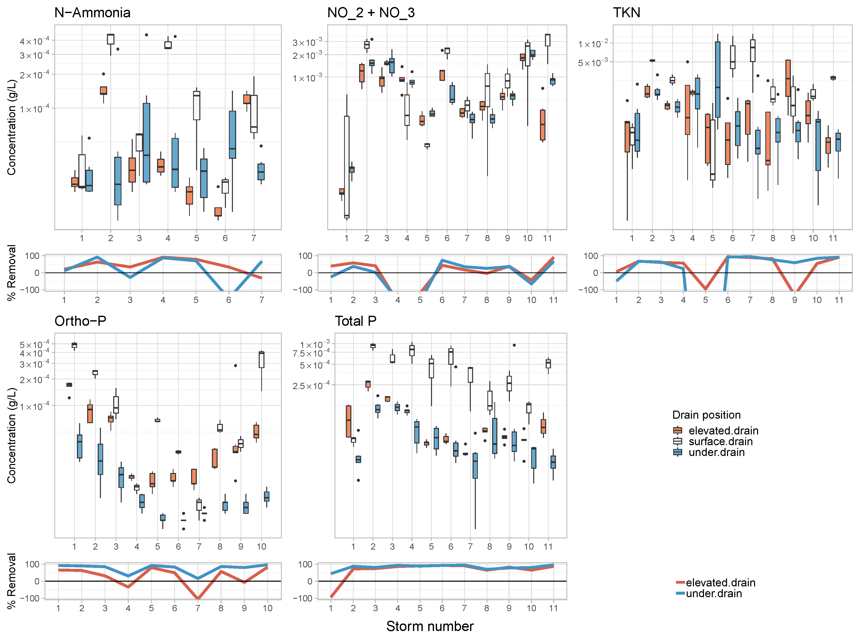
Of the nutrients evaluated, total phosphorous was removed at the highest level at both elevated drain and under drain positions. Median removal efficiencies across all storms was 82.7% and 87.7%, at the elevated drains and under drains, respectively. The geometric means of per storm concentrations were significantly different between surface versus elevated drains (Mann–Whitney statistic U = 0, p = 0.018) and surface versus under drains (U = 18, p = 0.014). Median removal efficiencies of ortho-P were highest at the under drain position (86.0%) and significantly different from surface samples (U = 18, p = 0.014). Ortho-P removal efficiency at the elevated drain was also significant (U = 0, p = 0.018) with a median removal efficiency of 53.4%. However, it is important to note that every nutrient analyte exhibited export at either the elevated drain, or the under drain for at least one storm event. In Figure 4, the lower row of sub-figures illustrates this issue where every analyte crosses the 0% removal (export) line at least once, with the exception of ortho-P and total P at the under drain position where there is removal across all storms. Both N-ammonia and Total Kjeldahl Nitrogen (TKN) were removed at significant levels at the under drain position, despite a large export of TKN at the under drain during Storm 5. TKN removal efficiency was also significant at the elevated drain. Median removal efficiencies, number of samples, and p-values associated with Mann–Whitney U-tests for the six nutrient analyte classes are presented in Table 2. Of all nutrients analyzed, total P was the most consistently removed across all storms and at both drain positions. None of the five nutrient analytes showed significant monotonic trends in removal efficiencies with system age.
3.4. Heavy Metals
The removal of metals by porous asphalt at the elevated drain was most pronounced for total Pb (96.3%) and total Zn (95.0%); both analyte concentrations were significantly different when compared to surface concentrations from IA cells. Total Pb and total Zn were also removed at the highest rates at the under drain position Figure 5; again, both analyte concentrations at the under drain were significantly different from surface IA samples. In the dissolved phase, dissolved Zn had a median removal efficiency of 85.5% across 12 storm events. Other dissolved metals fared relatively poorly in terms of removal efficiencies; most median removal efficiencies at both drain positions were below 50.0% with the exception of dissolved Zn and dissolved Pb. A listing of heavy metal removal efficiencies, p-values associated with the Mann–Whitney U-test, and the number of samples is presented in Table 2. Removal efficiencies of total Pb showed an increasingly monotonic trend with system age at both the elevated drain (Kendall’s Tau = 0.56, p = 0.01, Theil–Sen slope estimate = 0.42% increase per storm) and under drain ( = 0.51, p = 0.02, Theil–Sen slope estimate = 0.75% increase per storm). Total Zn also showed a low, but significant increasing trend in removal efficiencies with system age at the under drain ( = 0.61, p = 0.005, Theil–Sen slope estimate = 0.04% increase per storm).
3.5. Polycyclic Aromatic Hydrocarbons
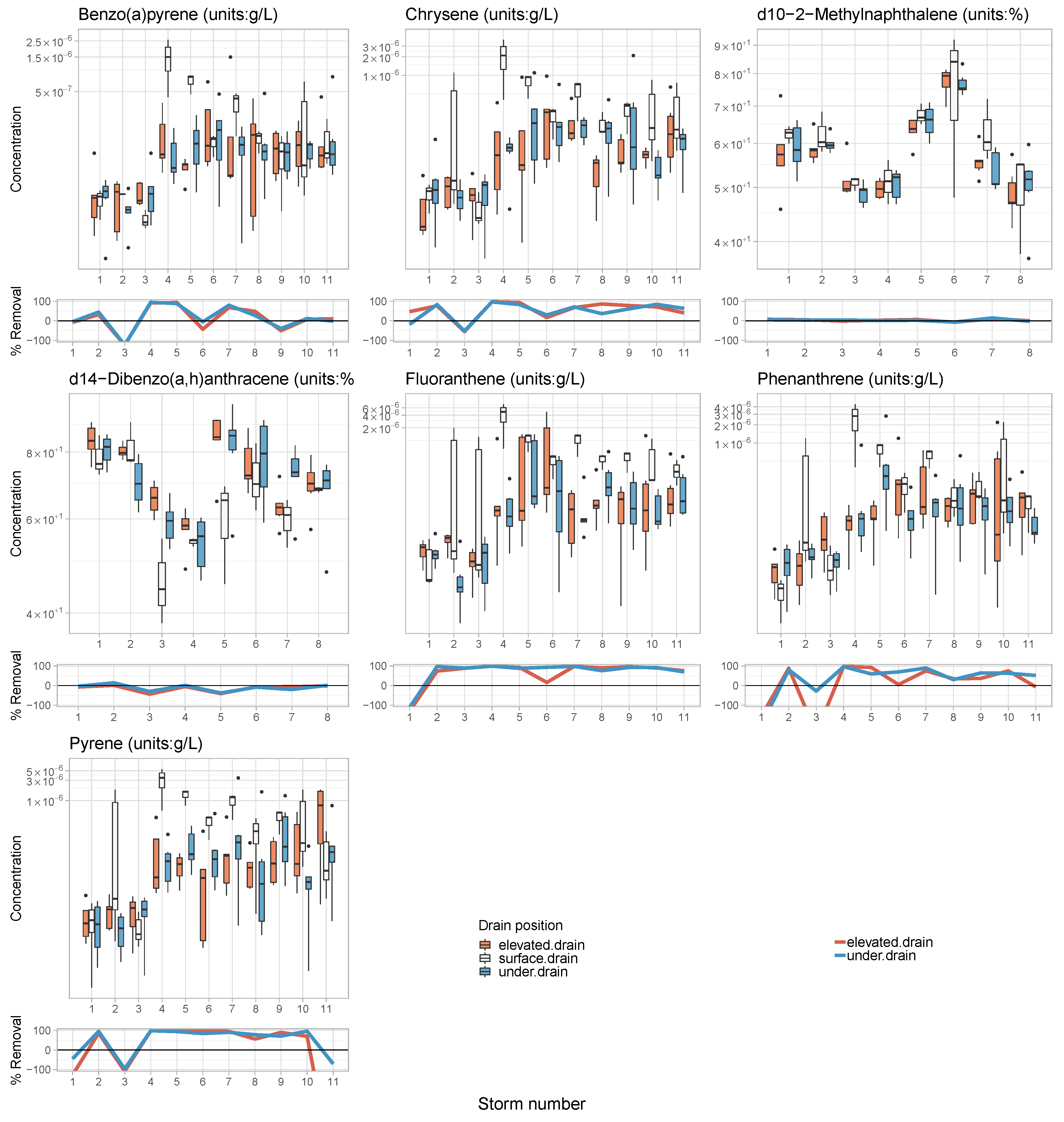
The two PAHs best removed by porous asphalt at the elevated drain were fluoranthene (89.9%) and pyrene (86.8%); however, neither analyte was significantly different from IA surface sample concentrations. Fluoranthene and pyrene also had the highest pollutant removal efficiencies at the under drain position, 91.8% and 84.6%, respectively. Both analyte concentrations at the under drain were significantly different from surface samples based on the Mann–Whitney U-test. The median removal efficiency for d14-dibenzo(a,h)anthracene was negative at both drains with only Storm 2 (Figure 6) exhibiting a nominal positive removal efficiency. A listing of all PAH removal rates, p-values associated with the Mann–Whitney U-test, and the number of samples from different drain position is presented in Table 2. None of the seven PAH analytes showed significant monotonic trends in removal efficiencies with system age.
3.6. Total Petroleum Hydrocarbons
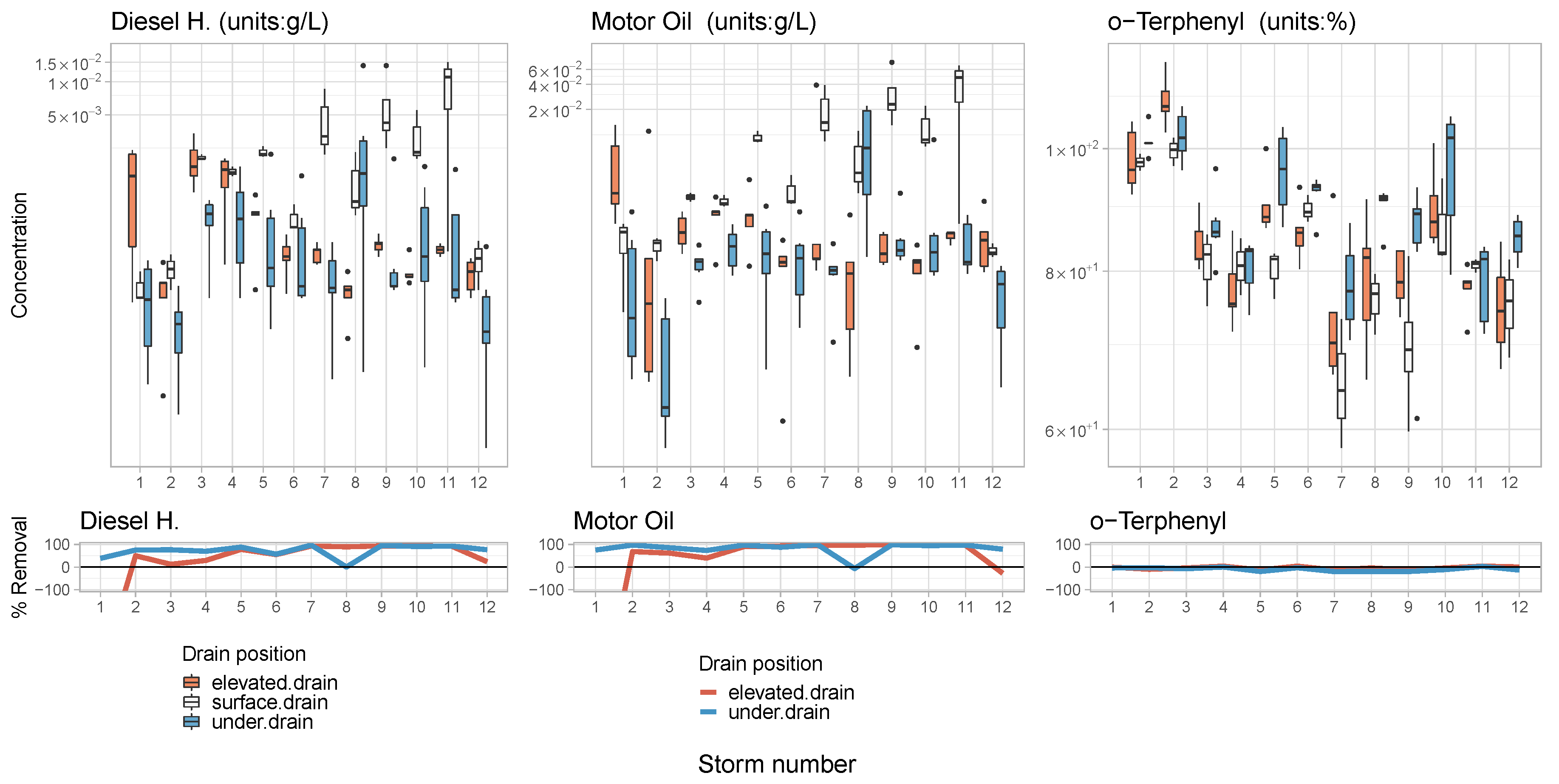
The highest median removal efficiency of any TPH analyte was motor oil, which was highest at both elevated drain and under drains, followed by diesel H.removal. The third highest removal of a TPH analyte was o-terphenyl which exhibited negative removal efficiencies (Figure 7) for all 12 storms at both elevated and under drain positions. Elevated drain and under drain samples from PA cells for both motor oil and diesel H. were significantly different from corresponding surface IA samples. These two analytes exhibited positive removal efficiencies for all sampled storms with the exception of Storm 1 when removal efficiencies for both analytes at the elevated drain position were below −400% (not shown in Figure 7). A listing of all TPH removal rates, p-values associated with the Mann–Whitney U-test, and number of samples from different drain positions, is presented in Table 2. Removal efficiencies of diesel H. showed an increasingly monotonic trend with system age at the under drain ( = 0.51, p = 0.02, Theil–Sen slope estimate = 0.10% increase per storm). Motor oil also exhibited a significantly increasing trend in removal efficiencies with system age, also at the under drain ( = 0.48, p = 0.03, Theil–Sen slope estimate = 0.06% increase per storm).
3.7. Stormwater Chemistry
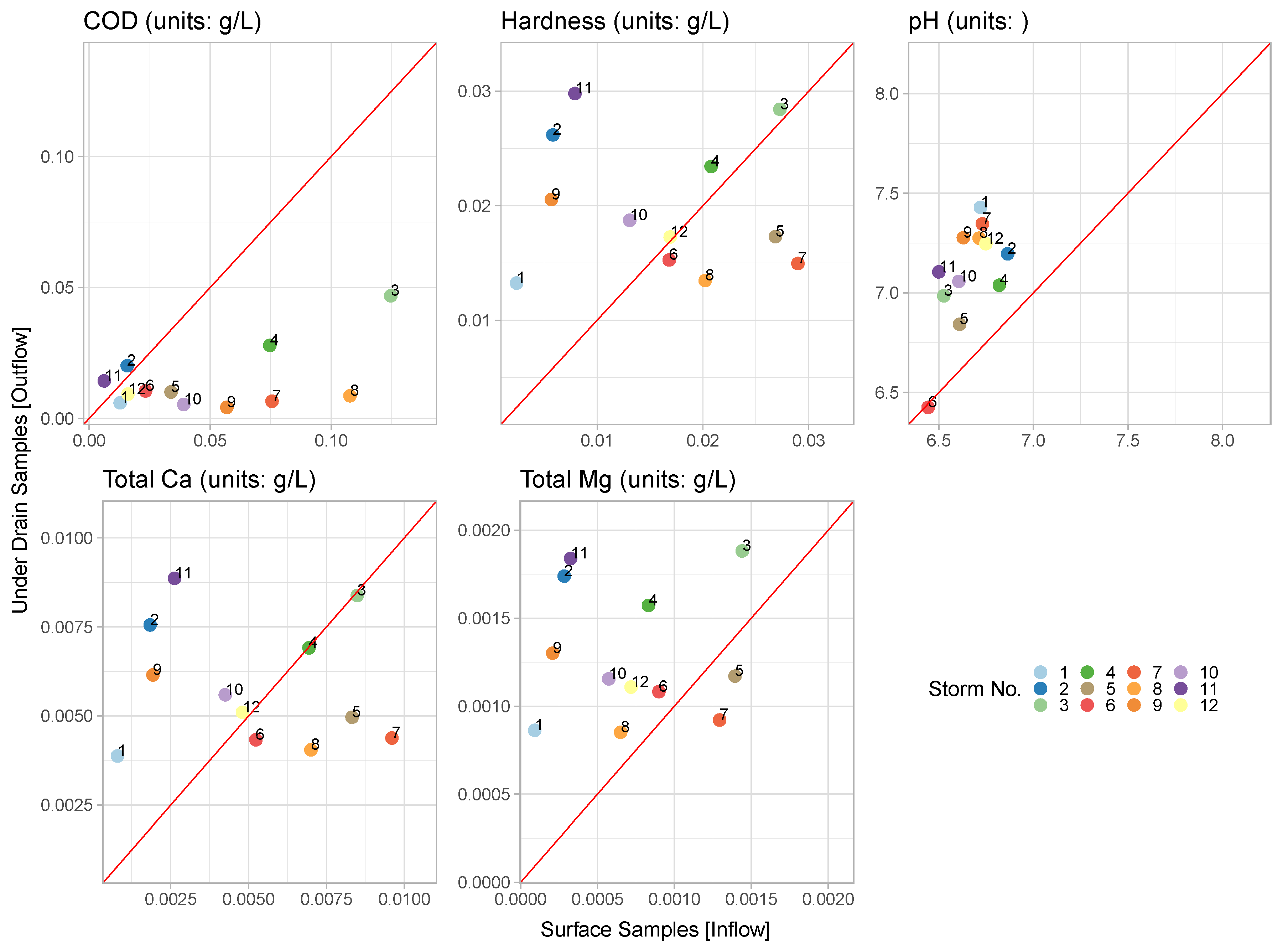
Changes in stormwater chemistry are described in terms of pH, COD, and hardness. COD between surface and elevated drain samples was significantly different, with COD almost 62.0% lower at the elevated drain compared to surface samples (Table 2). While neither hardness nor pH were significantly different, pH values at the under drain were consistently higher than samples at the surface for all but one of the 12 storms measured. The majority of total Mg samples at the under drain position showed analyte export, while the majority of total Ca samples reflected export or remained unchanged (Figure 8). Both analytes are described by negative values in terms of median removal rates (Table 2).
4. Discussion
4.1. Overall Performance
Pollutant removal efficiencies of all 33 stormwater analytes tested through this work and when viewed in totality (Figure 9) show that coarse sediments had the highest removal efficiency rates at both elevated drain (median removal: 99.5%, 95%-CI: 98.2–99.9%) and under drain positions (median removal: 98.7%, 95%-CI: 97.6–99.8%), followed by total Pb and total Zn. There was a clear relationship between analyte size or phase, and its removal when compared with its finer or dissolved-state analog. For example and expectedly, coarser sediment had better removal compared with fine sediment, and total metals removal was greater compared to removals of the corresponding dissolved forms. These results are consistent with [34], who found that coarser fractions of suspended sediment had higher removals from a porous asphalt test facility compared with finer fractions. The greater removal of particulate metals compared to the dissolved state was also demonstrated in a study by Pagotto et al. [50] where runoff from a conventional and porous asphalt systems was compared. These results suggest that filtration is likely a dominant process in the performance of porous asphalt systems, a result that was also suggested by Stotz and Krauth [32]. Additionally, the study of Pagotto et al. [50] also showed that total Pb, total Zn, and total Cd had considerably greater removals than total Cu, a result that is reflected in our study, as well. The differential removal of metals by porous asphalt systems is attributed to particulate affinity [31], where metals that are primarily in the particulate phase tend to adsorb to sediments that are trapped within the pavement system, and therefore removed from effluent stormwater. It was also clear that with the age of the system, removal efficiencies of total Pb, total Zn, diesel H., and motor oil improved by a small, but significant extents.
In terms of nutrient removal, the highest concentration of nitrogen species emanating from the IA surface drains was of the organic form (calculated by: organic-N = TKN − N-ammonia) and comprised approximately 68% of total nitrogen (calculated by: total N = TKN + nitrite + nitrate). Similarly, a greater fraction of organic-N was removed at the under drain position compared to removal of the inorganic fraction of total nitrogen. The high organic fraction of influent nitrogen and the greater removal of the organic form of nitrogen are consistent with a study by Drake et al. [51] on two kinds of interlocking permeable concrete pavements. However, per Brown and Borst [52], the relative abundance of organic nitrogen in the influent stormwater was wholly dependent on local traffic and site conditions, and is therefore not necessarily a generalizable result.
4.2. Maintenance
The effect of maintenance was not clearly discerned, with effluent sample concentrations from maintained cells indistinguishable from those measured from unmaintained cells. We hypothesize this result to be a function of the low annual cleaning frequency, low traffic conditions over the five-year study, and infrequent addition of street dirt over a five-year period. These results are also consistent with a stormwater quantity analysis [20] performed on the same system that did not find significant differences in infiltration rates between maintained and unmaintained PA cells. However, it is noteworthy that analytes with high removal efficiencies like sediments, total P, and motor oil were also analytes that had a propensity to appear in higher concentrations from the under drains of maintained cells, when compared with contemporaneous samples from unmaintained cells. In other words, the action of maintenance seemed to slightly inhibit the ability of a PA cell to remove certain pollutants. One possible hypothesis to explain this phenomenon is that while the porous asphalt systems retain particulate pollutants well, most of that retention occurs in the top wearing porous asphalt layer. With the action of annual maintenance by an air regenerative street sweeper, percussive blasts of air from the street sweeper designed to dislodge particulate matter deposited on the surface, actually force retained particulate matter downward through the porous asphalt wearing layer into the reservoir layer below. Once within the more permeable reservoir layer, these pollutants move more easily downward through the rocks and are eventually transported to the under drain. A simpler explanation is that suction by the vacuum hose opens surface pores enough to allow particulate contaminants to pass more easily compared with unmaintained cells where pores may be slightly more clogged. However, this would also mean that the maintained cells would have better infiltration rates, a phenomenon not supported by results reported by Knappenberger et al. [20]. It is also important to note that despite the low concrete curb between sample cells, the transfer of fines and materials from outside locations, and between maintained and unmaintained cells was not quantified and could have potentially confounded the determination of how influential maintenance was on pollutant removal efficiencies.
4.3. Ca and Mg Export
The increase in pH values in most samples from slightly acidic to slightly basic, between the surface drain and the under drain, highlights the buffering capacity of the granitic material used in the reservoir course [53], and of the porous asphalt system as a whole when granitic material is used in the reservoir course. Knauss and Wolery [54] showed that mineral quartz dissolution, a major mineral in granitic rocks, increases as pH levels in the water that the rock is in contact increase above a threshold value of six.
Several studies have shown that the dissolution of granite by water produces Mg and Ca cations through a complex relationship of rock–water interactions that are controlled by pH, temperature, pressure, and ionic concentrations in the aqueous solution [55,56,57,58,59,60]. A granite dissolution study by Chae et al. [61] showed that ionic Ca concentrations in leachate water in contact with granitic particles gradually increased over time. In another granite dissolution study by Savage et al. [62] where ionic concentrations of both Ca and Mg in leachate were measured, dissolution rates associated with Ca and Mg increased with a change in pH from 6.0–7.3. However, the rate of production of Mg cations (units: kg/m/s) through granite dissolution was a whole order of magnitude higher than for Ca cations over an identical change in pH. These studies are consistent with this work where both total Ca and total Mg export from the porous asphalt system was observed for a majority of the storms, accompanied by the observation that the relative increase in analyte concentration between surface drain and under drain was greater for total Mg.
4.4. Relevance to Stormwater BMP Performance Standards
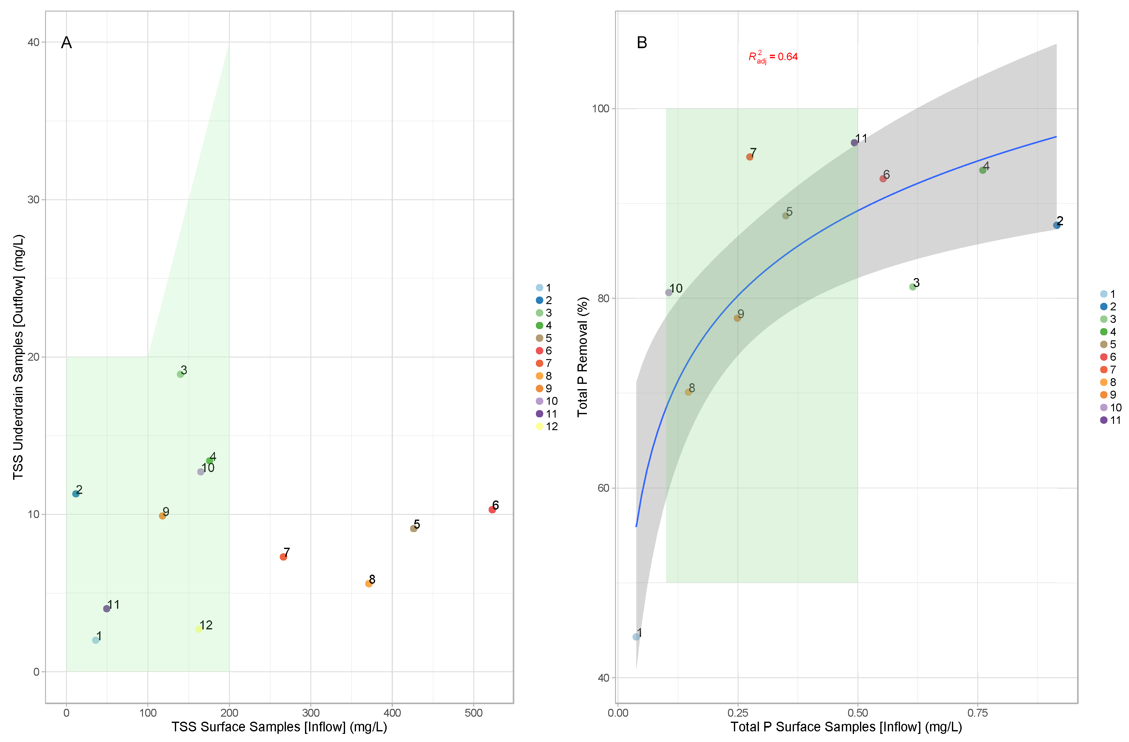
Median TSS removal, in fourth place (in Figure 9), was over 90.0% at both elevated drains (median removal: 97.3%, 95%-CI: 89.9–99.2%) and under drains (median removal: 93.4%, 95%-CI: 86.5–98.2%). Based on this work, porous asphalt pavements met the performance criteria for a primary treatment stormwater BMP in the states of Washington [9], New Jersey [63], New Hampshire [64], and North Carolina [65]. In Washington State, the criteria for this goal require TSS removal above 80.0% when inflows are > 100 and < 200 ; additionally, when inflows are below 100 , outflow concentrations must be below 20 [9]. Figure 10A illustrates this performance goal in relation to storms evaluated in this study. In fact, the maximum measured effluent TSS concentration was across all storms, and across all influent (surface) concentrations. Performance criteria for total P require removal above 50.0% for influent concentrations ranging from 0.1– . Total P in ninth place also showed reasonably good median removals (>80.0%) at both elevated drain and under drains; however, the 95.0% bootstrapped confidence intervals at the elevated drain (confidence interval: −1.7–90.3%) showed a wide range compared to the under drain position (95%-CI: 70.1–94.5%). The performance standard in Washington State is a removal of 50.0% provided that influent concentrations range between 0.1 and . The mean total P concentrations from the surface of IA cells (influent) fell within this range for six storms, with all six storms meeting the total P performance criteria (Figure 10B) at the under drain position. Storm 1 had the lowest mean surface sample concentration of , and the lowest pollutant removal efficiency at the under drain. An exponential regression curve explained over 64.0% of the variation in the data and suggested that total P removal increased with higher influent concentrations.
5. Conclusions
The ability of six porous asphalt pavement cells to remove stormwater pollutants was evaluated over five years by comparing analyte concentrations emanating from elevated drains and under drains, with corresponding concentrations from three proximal impervious asphalt surfaces. A minimum of seven storms and a maximum of 12 storm events were evaluated for pollutant removal efficiencies. The change in pollutant removal efficiency with the age of the cells, as well as the effect of maintenance on removal efficiencies were examined. It was shown that neither age nor the type of maintenance regime deployed had significant effects on a majority of pollutant removal efficiencies. However, removal efficiencies of total Pb, total Zn, motor oil, and diesel H. improved with the age of the system. Additional work is needed to examine if cleaning of the pavements at a higher than annual frequency would result in discernible differences of effluent concentrations. There is also the possibility that air-regenerative sweepers exacerbate the movement of pollutants through the upper wearing course, also a topic for future examination. Porous asphalt pavements appear to act as large filtration systems, with particulate pollutants removed at the highest rates. Performance standards for TSS and TP removal stipulated by several states were met for the majority of storms examined. Granitic rock used for the subsurface aggregate course appeared to influence the chemistry of stormwater emanating from the porous asphalt cells. Further work is clearly necessitated to determine how basaltic rock or other added materials might influence effluent chemistry. A final area of critically needed future work is the role of biotic processes underway within the upper wearing coarse and lower aggregate courses. Mosses are frequently seen in the interstitial spaces of the upper wearing course, elucidating microbial and other processes associated with contaminant breakdown would inform maintenance frequencies, given that maintenance typically removes moss.
Author Contributions
Conceptualization, C.H. and J.S.; methodology, A.J., T.K., and C.H.; software, A.J. and T.K.; validation, A.J. and T.K.; formal analysis, A.J. and T.K.; investigation, A.J.; resources, J.S.; data curation, T.K.; writing, original draft preparation, A.J.; writing, review and editing, A.J., T.K., J.S., and C.H.; visualization, A.J.; supervision, A.J.; project administration, J.S.; funding acquisition, J.S. and C.H.
Funding
This research was funded by the Puget Sound National Estuary Program (NEP) Watershed Grant Program Grant Number G1200452.
Acknowledgments
Our complete gratitude to technicians Richard Bembenek and Carly Thompson, who played crucial roles in data collection. Thanks to MIG|SvR for design, engineering and permitting of the test pavements, and for blending the rigors of research compliance with functional aesthetics for the visiting public. Lastly, huge thanks to Tanyalee Erwin, the former Asst. Director of the Washington Stormwater Center, her vision and leadership made much of this work possible.
Conflicts of Interest
The authors declare no conflicts of interest. The funders reviewed the design of the study to ensure that performance goal criteria for stormwater BMPs as defined by the Washington State Department of Ecology were likely to be met. The funders had no role in data collection, analyses, or interpretation of the data; in the writing of the manuscript; nor in the decision to publish the results.
Abbreviations
The following abbreviations are used in this manuscript:
| BMP | Best Management Practice |
| COD | Chemical Oxygen Demand |
| GSI | Green Stormwater Infrastructure |
| IA | Impervious Asphalt |
| OGFC | Open-Graded Friction Course |
| PA | Porous Asphalt |
| PAH | Polycyclic Aromatic Hydrocarbon |
| ROS | Regression on Order Statistics |
| TKN | Total Kjeldahl Nitrogen |
| TP | Total Phosphorous |
| TPH | Total Petroleum Hydrocarbon |
| TSS | Total Suspended Solids |
References
- Puget Sound Action Team. The State of the Sound; Technical Report; Puget Sound Partnership: Tacoma, WA, USA, 2007.
- Grumbes, B.H. Using Green Infrastructure to Protect Water Quality in Stormwater, CSO, Nonpoint Source and Other Water Programs; Technical Report; United States Environmental Protection Agency (EPA): Washington, DC, USA, 2007.
- Fletcher, T.D.; Shuster, W.; Hunt, W.F.; Ashley, R.; Butler, D.; Arthur, S.; Trowsdale, S.; Barraud, S.; Semadeni-Davies, A.; Bertrand-Krajewski, J.L.; et al. SUDS, LID, BMPs, WSUD and more—The evolution and application of terminology surrounding urban drainage. Urb. Water J. 2015, 12, 525–542. [Google Scholar] [CrossRef]
- Askarizadeh, A.; Rippy, M.A.; Fletcher, T.D.; Feldman, D.L.; Peng, J.; Bowler, P.; Mehring, A.S.; Winfrey, B.K.; Vrugt, J.A.; AghaKouchak, A.; et al. From rain tanks to catchments: Use of low-impact development to address hydrologic symptoms of the urban stream syndrome. Environ. Sci. Technol. 2015, 49, 11264–11280. [Google Scholar] [CrossRef] [PubMed]
- Pataki, D.E.; Carreiro, M.M.; Cherrier, J.; Grulke, N.E.; Jennings, V.; Pincetl, S.; Pouyat, R.V.; Whitlow, T.H.; Zipperer, W.C. Coupling biogeochemical cycles in urban environments: Ecosystem services, green solutions, and misconceptions. Front. Ecol. Environ. 2011, 9, 27–36. [Google Scholar] [CrossRef]
- Lucas, W.C.; Sample, D.J. Reducing combined sewer overflows by using outlet controls for Green Stormwater Infrastructure: Case study in Richmond, Virginia. J. Hydrol. 2015, 520, 473–488. [Google Scholar] [CrossRef]
- Pennino, M.J.; McDonald, R.I.; Jaffe, P.R. Watershed-scale impacts of stormwater green infrastructure on hydrology, nutrient fluxes, and combined sewer overflows in the mid-Atlantic region. Sci. Total Environ. 2016, 565, 1044–1053. [Google Scholar] [CrossRef] [PubMed] [Green Version]
- Miles, B.; Band, L.E. Green infrastructure stormwater management at the watershed scale: Urban variable source area and watershed capacitance. Hydrol. Process. 2015, 29, 2268–2274. [Google Scholar] [CrossRef]
- Washington State Department of Ecology. Stormwater Management Manual for Western Washington (SWMMWW); Washington State Department of Ecology: Lacey, WA, USA, 2014.
- Drake, J.A.P.; Bradford, A.; Marsalek, J. Review of environmental performance of permeable pavement systems: state of the knowledge. Water Qual. Res. J. Can. 2013, 48, 203–222. [Google Scholar] [CrossRef]
- Fassman, E.A.; Blackbourn, S. Urban runoff mitigation by a permeable pavement system over impermeable soils. J. Hydrol. Eng. 2010, 15, 475–485. [Google Scholar] [CrossRef]
- United States Environmental Protection Agency. Stormwater Technology Fact Sheet: Porous Pavement; United States Environmental Protection Agency: Washington, DC, USA, 1999.
- Collins, K.A.; Hunt, W.F.; Hathaway, J.M. Hydrologic comparison of four types of permeable pavement and standard asphalt in eastern North Carolina. J. Hydrol. Eng. 2008, 13, 1146–1157. [Google Scholar] [CrossRef]
- Dietz, M.E. Low impact development practices: A review of current research and recommendations for future directions. Water Air Soil Pollut. 2007, 186, 351–363. [Google Scholar] [CrossRef]
- Roseen, R.M.; Ballestero, T.P.; Houle, J.J.; Briggs, J.F.; Houle, K.M. Water quality and hydrologic performance of a porous asphalt pavement as a storm-water treatment strategy in a cold climate. J. Environ. Eng. 2011, 138, 81–89. [Google Scholar] [CrossRef]
- Scholz, M.; Grabowiecki, P. Review of permeable pavement systems. Build. Environ. 2007, 42, 3830–3836. [Google Scholar] [CrossRef]
- Al-Rubaei, A.M.; Stenglein, A.L.; Viklander, M.; Blecken, G.T. Long-term hydraulic performance of porous asphalt pavements in northern Sweden. J. Irrig. Drain. Eng. 2013, 139, 499–505. [Google Scholar] [CrossRef]
- Hinman, C. Low Impact Development: Technical Guidance Manual for Puget Sound; Puget Sound Action Team: Tacoma, WA, USA, 2005.
- Ahiablame, L.M.; Engel, B.A.; Chaubey, I. Effectiveness of low impact development practices: Literature review and suggestions for future research. Water Air Soil Pollut. 2012, 223, 4253–4273. [Google Scholar] [CrossRef]
- Knappenberger, T.; Jayakaran, A.D.; Stark, J.D.; Hinman, C.H. Monitoring porous assphalt stormwater infiltration and outflow. J. Irrig. Drain. Eng. 2017, 143, 04017027. [Google Scholar] [CrossRef]
- Bean, E.Z.; Hunt, W.F.; Bidelspach, D.A. Field survey of permeable pavement surface infiltration rates. J. Irrig. Drain. Eng. 2007, 133, 249–255. [Google Scholar] [CrossRef]
- Brinkmann, W. Urban stormwater pollutants: Sources and loadings. GeoJournal 1985, 11, 277–283. [Google Scholar] [CrossRef]
- Malmqvist, P.A. Urban Stormwater Pollutant Sources—An Analysis of Inflows and Outflows of Nitrogen, Phosphorus, Lead, Zinc and Copper in Urban Areas; Chalmers University of Technology: Göteborg, Sweden, 1983. [Google Scholar]
- Chow, M.; Yusop, Z. Characterization and source identification of stormwater runoff in tropical urban catchments. Water Sci. Technol. 2014, 69, 244–252. [Google Scholar] [CrossRef]
- Pitt, R.; Field, R.; Lalor, M.; Brown, M. Urban stormwater toxic pollutants: Assessment, sources, and treatability. Water Environ. Res. 1995, 67, 260–275. [Google Scholar] [CrossRef]
- Lee, J.H.; Bang, K.W. Characterization of urban stormwater runoff. Water Res. 2000, 34, 1773–1780. [Google Scholar] [CrossRef]
- Du, B.; Lofton, J.M.; Peter, K.T.; Gipe, A.D.; James, C.A.; McIntyre, J.K.; Scholz, N.L.; Baker, J.E.; Kolodziej, E.P. Development of suspect and non-target screening methods for detection of organic contaminants in highway runoff and fish tissue with high-resolution time-of-flight mass spectrometry. Environ. Sci. Process. Impacts 2017, 19, 1185–1196. [Google Scholar] [CrossRef]
- Pratt, C.; Newman, A.; Bond, P. Mineral oil bio-degradation within a permeable pavement: Long term observations. Water Sci. Technol. 1999, 39, 103–109. [Google Scholar] [CrossRef]
- Simon Beecham, G.; BE, D.P. Stormwater treatment using permeable pavements. Proc. Inst. Civ. Eng. 2012, 165, 161. [Google Scholar]
- Imran, H.; Akib, S.; Karim, M.R. Permeable pavement and stormwater management systems: A review. Environ. Technol. 2013, 34, 2649–2656. [Google Scholar] [CrossRef] [PubMed]
- Zhang, K.; Yong, F.; McCarthy, D.T.; Deletic, A. Predicting long term removal of heavy metals from porous pavements for stormwater treatment. Water Res. 2018, 142, 236–245. [Google Scholar] [CrossRef] [PubMed]
- Stotz, G.; Krauth, K. The pollution of effluents from pervious pavements of an experimental highway section: First results. Sci. Total Environ. 1994, 146, 465–470. [Google Scholar] [CrossRef]
- Tota-Maharaj, K.; Scholz, M. Efficiency of permeable pavement systems for the removal of urban runoff pollutants under varying environmental conditions. Environ. Prog. Sustain. Energy 2010, 29, 358–369. [Google Scholar] [CrossRef]
- Brown, C.; Chu, A.; van Duin, B.; Valeo, C. Characteristics of sediment removal in two types of permeable pavement. Water Qual. Res. J. 2009, 44, 59. [Google Scholar] [CrossRef]
- Baladès, J.D.; Legret, M.; Madiec, H. Permeable pavements: Pollution management tools. Water Sci. Technol. 1995, 32, 49–56. [Google Scholar] [CrossRef]
- Hammes, G.; Thives, L.P.; Ghisi, E. Application of stormwater collected from porous asphalt pavements for non-potable uses in buildings. J. Environ. Manag. 2018, 222, 338–347. [Google Scholar] [CrossRef]
- Kumar, K.; Kozak, J.; Hundal, L.; Cox, A.; Zhang, H.; Granato, T. In-situ infiltration performance of different permeable pavements in a employee used parking lot—A four-year study. J. Environ. Manag. 2016, 167, 8–14. [Google Scholar] [CrossRef] [PubMed]
- Sansalone, J.; Kuang, X.; Ying, G.; Ranieri, V. Filtration and clogging of permeable pavement loaded by urban drainage. Water Res. 2012, 46, 6763–6774. [Google Scholar] [CrossRef] [PubMed]
- Radfar, A.; Rockaway, T.D. Clogging prediction of permeable pavement. J. Irrig. Drain. Eng. 2016, 142, 04015069. [Google Scholar] [CrossRef]
- Winston, R.J.; Al-Rubaei, A.M.; Blecken, G.T.; Viklander, M.; Hunt, W.F. Maintenance measures for preservation and recovery of permeable pavement surface infiltration rate—The effects of street sweeping, vacuum cleaning, high pressure washing, and milling. J. Environ. Manag. 2016, 169, 132–144. [Google Scholar] [CrossRef]
- Breault, R.F.; Smith, K.P.; Sorenson, J.R. Residential Street-Dirt Accumulation Rates and Chemical Composition, and Removal Efficiencies by Mechanical-and Vacuum-Type Sweepers, New Bedford, Massachusetts, 2003–2004; Technical Report 4; US Geological Survey: Reston, VA, USA, 2005.
- Sehgal, K.; Drake, J.; Seters, T.; Vander Linden, W. Improving restorative maintenance practices for mature permeable interlocking concrete pavements. Water 2018, 10, 1588. [Google Scholar] [CrossRef]
- Washington State Department of Ecology. Technical Guidance Manual for Evaluating Emerging Stormwater Treatment Technologies; Technology Assessment Protocol—Ecology (TAPE); Washington State Department of Ecology: Lacey, WA, USA, 2011.
- Seattle Public Utilities; Herrera Environment Consultants. Seattle Street Sweeping Pilot Study—Monitoring Report; Techreport; Seattle Public Utilities: Seattle, WA, USA, 2009.
- R Core Team. R: A Language and Environment for Statistical Computing; R Foundation for Statistical Computing: Vienna, Austria, 2018. [Google Scholar]
- Nachar, N. The Mann–Whitney U: A test for assessing whether two independent samples come from the same distribution. Tutor. Quant. Methods Psychol. 2008, 4, 13–20. [Google Scholar] [CrossRef]
- Helsel, D.R. Statistics for Censored Environmental Data Using Minitab and R; John Wiley & Sons: Hoboken, NJ, USA, 2011; pp. 1–19. [Google Scholar]
- Theil, H. A rank-invariant method of linear and polynomial regression analysis. In Henri Theil’s Contributions to Economics and Econometrics; Springer: Berlin, Germany, 1992; pp. 345–381. [Google Scholar]
- Sen, P.K. Estimates of the regression coefficient based on Kendall’s tau. J. Am. Stat. Assoc. 1968, 63, 1379–1389. [Google Scholar] [CrossRef]
- Pagotto, C.; Legret, M.; Le Cloirec, P. Comparison of the hydraulic behaviour and the quality of highway runoff water according to the type of pavement. Water Res. 2000, 34, 4446–4454. [Google Scholar] [CrossRef]
- Drake, J.; Bradford, A.; Van Seters, T. Stormwater quality of spring-summer-fall effluent from three partial-infiltration permeable pavement systems and conventional asphalt pavement. J. Environ. Manag. 2014, 139, 69–79. [Google Scholar] [CrossRef]
- Brown, R.A.; Borst, M. Nutrient infiltrate concentrations from three permeable pavement types. J. Environ. Manag. 2015, 164, 74–85. [Google Scholar] [CrossRef] [Green Version]
- Ré, C.L.; Kaszuba, J.P.; Moore, J.N.; McPherson, B.J. Fluid-rock interactions in CO2-saturated, granite-hosted geothermal systems: Implications for natural and engineered systems from geochemical experiments and models. Geochim. Cosmochim. Acta 2014, 141, 160–178. [Google Scholar]
- Knauss, K.G.; Wolery, T.J. The dissolution kinetics of quartz as a function of pH and time at 70 C. Geochim. Cosmochim. Acta 1988, 52, 43–53. [Google Scholar] [CrossRef]
- Richards, H.G.; Savage, D.; Andrews, J.N. Granite-water reactions in an experimental Hot Dry Rock geothermal reservoir, Rosemanowes test site, Cornwall, UK. Appl. Geochem. 1992, 7, 193–222. [Google Scholar] [CrossRef]
- Nekvasil, H.; Burnham, C.W. The calculated individual effects of pressure and water content on phase equilibria in the granite system. In Magmatic Processes: Physicochemical Principles; Lancaster Press: Lancaster, UK, 1987; Volume 1, pp. 433–445. [Google Scholar]
- Trimmer, D.; Bonner, B.; Heard, H.; Duba, A. Effect of pressure and stress on water transport in intact and fractured gabbro and granite. J. Geophys. Res. Solid Earth 1980, 85, 7059–7071. [Google Scholar] [CrossRef]
- Lu, R.; Watanabe, N.; He, W.; Jang, E.; Shao, H.; Kolditz, O.; Shao, H. Calibration of water-granite interaction with pressure solution in a flow-through fracture under confining pressure. Environ. Earth Sci. 2017, 76, 417. [Google Scholar] [CrossRef]
- Miao, S.; Cai, M.; Guo, Q.; Wang, P.; Liang, M. Damage effects and mechanisms in granite treated with acidic chemical solutions. Int. J. Rock Mech. Min. Sci. 2016, 88, 77–86. [Google Scholar] [CrossRef]
- Worley, W.G. Dissolution Kinetics and Mechanisms in Quartz-and Grainite-Water Systems. Ph.D. Thesis, Massachusetts Institute of Technology, Cambridge, MA, USA, 1994. [Google Scholar]
- Chae, G.T.; Yun, S.T.; Kwon, M.J.; Kim, Y.S.; Mayer, B. Batch dissolution of granite and biotite in water: Implication for fluorine geochemistry in groundwater. Geochem. J. 2006, 40, 95–102. [Google Scholar] [CrossRef] [Green Version]
- Savage, D.; Bateman, K.; Richards, H.G. Granite-water interactions in a flow-through experimental system with applications to the Hot Dry Rock geothermal system at Rosemanowes, Cornwall, UK. Appl. Geochem. 1992, 7, 223–241. [Google Scholar] [CrossRef]
- New Jersey Department of Environmental Protection. NJ Stormwater Best Management Practices Manual; New Jersey Department of Environmental Protection: Trenton, NJ, USA, 2018.
- New Hampshire Department of Enivronmental Services. New Hampshire Stormwater Manual; New Hampshire Department of Enivronmental Services: Concord, NC, USA, 2008; Volume 1.
- North Carolina Environmental Quality. NCDEQ Stormwater Design Manual; North Carolina Environmental Quality: Raleigh, NC, USA, 2017.
Figure 1.
(A) Site plan of the porous asphalt cells. Maintained cells were cleaned annually with a regenerative air street sweeper. (B) Dimensions of each test cell. The dashed line (A-A) shows the cross-section locations of porous asphalt (C) and impervious asphalt (D) cells.
Figure 1.
(A) Site plan of the porous asphalt cells. Maintained cells were cleaned annually with a regenerative air street sweeper. (B) Dimensions of each test cell. The dashed line (A-A) shows the cross-section locations of porous asphalt (C) and impervious asphalt (D) cells.

Figure 2.
Boxplots show the distributions of geometric means of TSS concentrations for 12 storms, grouped by cell maintenance regime and drain position. Effluent concentrations from the surface of Impervious Asphalt (IA) cells served as the study control.
Figure 2.
Boxplots show the distributions of geometric means of TSS concentrations for 12 storms, grouped by cell maintenance regime and drain position. Effluent concentrations from the surface of Impervious Asphalt (IA) cells served as the study control.

Figure 3.
Effluent concentrations for coarse, fine, and total suspended solids grouped by storm and drain position [upper row]. The lower panel shows pollutant removal efficiencies across all measured storms. Removal efficiencies plotting below the 0% removal efficiency line illustrate sediment-exporting storm events (e.g., fine sediment: Storms 7 and 9 at the under drain)Sediments across all storms and removal efficiencies.

Figure 4.
Effluent concentrations for nitrite + nitrate, ammonia, total Kjeldahl N, total P, and ortho-P grouped by storm and drain position [upper row]. The lower panel shows pollutant removal efficiencies across all measured storms. Removal efficiency for TKN-Storm 5 (under drain) was below −100% (or over 100% export) and is not shown.

Figure 5.
Removal efficiencies for total and dissolved heavy metals at elevated drain and under drain positions. Removal efficiencies below −100% (or over 100% export) are not shown, and why some line graphs appear broken.
Figure 5.
Removal efficiencies for total and dissolved heavy metals at elevated drain and under drain positions. Removal efficiencies below −100% (or over 100% export) are not shown, and why some line graphs appear broken.

Figure 6.
Removal efficiencies for PAHs at elevated drain and under drain positions across measured storms. Removal efficiencies below −100% (or over 100% export) are not shown, and why some line graphs appear broken.
Figure 6.
Removal efficiencies for PAHs at elevated drain and under drain positions across measured storms. Removal efficiencies below −100% (or over 100% export) are not shown, and why some line graphs appear broken.

Figure 7.
Removal efficiencies for TPHs at elevated drain and under drain positions across measured storms. Removal efficiencies below −100% (or over 100% export) are not shown, and why Storm 1 elevated drain removals for diesel H. and motor oil are not shown.
Figure 7.
Removal efficiencies for TPHs at elevated drain and under drain positions across measured storms. Removal efficiencies below −100% (or over 100% export) are not shown, and why Storm 1 elevated drain removals for diesel H. and motor oil are not shown.

Figure 8.
Comparisons of stormwater chemistry between outflow at the under drain position, and inflow (or stormwater from the surface of IA cells). Concentrations associated with storm events that plot above the 1:1 line (red line) suggest analyte export, while those below denote analyte removal.
Figure 8.
Comparisons of stormwater chemistry between outflow at the under drain position, and inflow (or stormwater from the surface of IA cells). Concentrations associated with storm events that plot above the 1:1 line (red line) suggest analyte export, while those below denote analyte removal.

Figure 9.
Median removal efficiencies for all analytes ordered from left to right by magnitude of removal at the under drain. Boot strapped confidence intervals for only under drain removals are shown. Only confidence intervals between −100% and 50% are shown.
Figure 9.
Median removal efficiencies for all analytes ordered from left to right by magnitude of removal at the under drain. Boot strapped confidence intervals for only under drain removals are shown. Only confidence intervals between −100% and 50% are shown.

Figure 10.
Effluent sample concentrations for TSS (A) and removal efficiencies for total P (B) at the under drain, versus mean IA surface concentrations (inflow) over storms. Light green regions represent bounding areas that define performance criteria for a stormwater BMP in order to meet the primary (TSS) and phosphorous treatment performance goals in the State of Washington. Storm events are represented by numbered dots.


Table 1.
List of storm dates, rainfall totals, and the type of pollutant load. Dosed events are those where spiked analyte solution was applied to the pavements prior to a storm. Synthetic storms were artificial events generated through the application of irrigation water to the pavements.
Table 1.
List of storm dates, rainfall totals, and the type of pollutant load. Dosed events are those where spiked analyte solution was applied to the pavements prior to a storm. Synthetic storms were artificial events generated through the application of irrigation water to the pavements.
| Storm No. | Date | Storm Type | Treatment | Rainfall/Irrigated Total (mm) |
|---|---|---|---|---|
| 1 | 18-11-2012 | Natural | Undosed | 47.8 |
| 2 | 22-02-2013 | Natural | Undosed | 9.4 |
| 3 | 30-07-2013 | Synthetic | Dosed | 30.6 |
| 4 | 13-08-2013 | Synthetic | Dosed | 33.1 |
| 5 | 08-10-2013 | Synthetic | Dosed | 32.1 |
| 6 | 22-10-2013 | Synthetic | Undosed | 34.0 |
| 7 | 05-03-2014 | Natural | Dosed | 17.0 |
| 8 | 15-03-2014 | Natural | Dosed | 32.5 |
| 9 | 17-04-2014 | Natural | Dosed | 19.8 |
| 10 | 30-10-2014 | Natural | Dosed | 26.2 |
| 11 | 25-10-2015 | Natural | Dosed | 16.8 |
| 12 | 12-11-2015 | Natural | Dosed | 53.3 |
Table 2.
Removal efficiencies of sediments by porous asphalt. Removal efficiencies calculated on a per storm basis, with median removal efficiency at two drain positions reported below. Samples were collected at three drain positions, surface (IA cells only), elevated, and under (PA cells only). Geometric Means (GM) reported in this table were calculated using pooled values across all storms.
| Analyte | Median Removal Elevated (%) | p-Value * | Median Removal Under (%) | p-Value * | N Surf | N Elev | N Under | N Storms | Units | Group | GM Surf | GM Elev | GM Under |
|---|---|---|---|---|---|---|---|---|---|---|---|---|---|
| Coarse Sed. | 99.5 | 0.016 | 98.7 | 0.014 | 27 | 46 | 52 | 9 | g/L | sediment | 2.38 | 7.98 | 1.96 |
| Fine Sed. | 59.4 | 0.018 | 57.0 | 0.123 | 27 | 46 | 52 | 9 | g/L | sediment | 1.12 | 3.62 | 5.09 |
| TSS | 97.3 | 0.018 | 93.4 | 0.014 | 36 | 62 | 69 | 12 | g/L | sediment | 1.35 | 3.82 | 7.46 |
| N-Ammonia | 34.1 | 0.117 | 68.0 | 0.014 | 21 | 35 | 42 | 7 | g/L | nutrient | 8.17 | 3.54 | 3.45 |
| NO_2 + NO_3 | 38.3 | 0.089 | 26.1 | 0.259 | 33 | 57 | 65 | 11 | g/L | nutrient | 6.39 | 4.76 | 5.47 |
| TKN | 61.0 | 0.018 | 67.4 | 0.014 | 33 | 57 | 66 | 11 | g/L | nutrient | 1.62 | 5.46 | 5.64 |
| Ortho-P | 53.4 | 0.018 | 86.0 | 0.014 | 30 | 52 | 59 | 10 | g/L | nutrient | 6.38 | 3.44 | 9.80 |
| Total P | 82.7 | 0.018 | 87.7 | 0.014 | 33 | 57 | 62 | 11 | g/L | nutrient | 2.98 | 6.16 | 3.69 |
| Diss. Cd | 20.9 | 0.500 | 13.6 | 0.409 | 36 | 62 | 70 | 12 | g/L | metal | 4.79 | 2.17 | 2.63 |
| Total Cd | 89.4 | 0.044 | 90.4 | 0.020 | 36 | 62 | 69 | 12 | g/L | metal | 2.97 | 3.79 | 3.32 |
| Diss. Cr | 26.2 | 0.131 | 36.0 | 0.096 | 35 | 62 | 70 | 12 | g/L | metal | 4.47 | 2.94 | 2.57 |
| Total Cr | 78.9 | 0.018 | 79.7 | 0.014 | 36 | 62 | 70 | 12 | g/L | metal | 2.35 | 4.11 | 4.96 |
| Diss. Cu | 26.9 | 0.091 | 44.4 | 0.014 | 35 | 62 | 70 | 12 | g/L | metal | 3.75 | 2.96 | 2.20 |
| Total Cu | 81.0 | 0.018 | 82.8 | 0.014 | 36 | 62 | 70 | 12 | g/L | metal | 1.98 | 3.27 | 2.90 |
| Diss. Pb | 56.8 | 0.036 | 79.6 | 0.021 | 35 | 62 | 70 | 12 | g/L | metal | 2.65 | 1.22 | 9.15 |
| Total Pb | 96.3 | 0.017 | 98.3 | 0.013 | 36 | 62 | 70 | 12 | g/L | metal | 9.88 | 4.03 | 2.38 |
| Diss. Zn | 85.5 | 0.018 | 91.3 | 0.014 | 35 | 62 | 70 | 12 | g/L | metal | 2.27 | 4.14 | 2.73 |
| Total Zn | 95.0 | 0.018 | 97.8 | 0.014 | 36 | 62 | 70 | 12 | g/L | metal | 1.04 | 5.07 | 3.74 |
| d10-2-Methyl. | 4.2 | 0.231 | 3.1 | 0.302 | 24 | 42 | 47 | 8 | % | PAH | 5.91 | 5.69 | 5.74 |
| Benzo(a)pyrene | 10.6 | 0.349 | 11.6 | 0.725 | 31 | 57 | 66 | 11 | g/L | PAH | 9.41 | 5.05 | 4.70 |
| Chrysene | 71.0 | 0.186 | 63.2 | 0.183 | 33 | 56 | 66 | 11 | g/L | PAH | 1.38 | 3.77 | 4.60 |
| d14-Dibenzo(a,h). | −6.2 | 0.850 | −5.7 | 0.819 | 24 | 42 | 47 | 8 | % | PAH | 6.35 | 7.13 | 6.93 |
| Fluoranthene | 89.9 | 0.097 | 91.8 | 0.018 | 33 | 57 | 66 | 11 | g/L | PAH | 1.41 | 1.64 | 1.21 |
| Phenanthrene | 36.6 | 0.383 | 62.9 | 0.383 | 33 | 57 | 66 | 11 | g/L | PAH | 1.17 | 4.72 | 4.23 |
| Pyrene | 86.8 | 0.383 | 84.6 | 0.078 | 33 | 57 | 66 | 11 | g/L | PAH | 7.61 | 1.63 | 1.38 |
| Diesel H. | 66.6 | 0.068 | 76.4 | 0.049 | 37 | 60 | 71 | 12 | g/L | TPH | 1.19 | 3.31 | 2.13 |
| Motor Oil | 91.3 | 0.018 | 91.2 | 0.014 | 37 | 60 | 70 | 12 | g/L | TPH | 3.35 | 4.71 | 2.68 |
| o-Terphenyl | −3.8 | 0.770 | −9.1 | 0.964 | 36 | 60 | 70 | 12 | % | TPH | 8.04 | 8.42 | 8.87 |
* p-Values denote significance of the Mann–Whitney U-statistic that tested differences between surface samples from IA cells and elevated drain and under drain samples from PA cells. † Surf = Surface; Elev = Elevated.
© 2019 by the authors. Licensee MDPI, Basel, Switzerland. This article is an open access article distributed under the terms and conditions of the Creative Commons Attribution (CC BY) license (http://creativecommons.org/licenses/by/4.0/).
Share and Cite
MDPI and ACS Style
Jayakaran, A.D.; Knappenberger, T.; Stark, J.D.; Hinman, C. Remediation of Stormwater Pollutants by Porous Asphalt Pavement. Water 2019, 11, 520. https://doi.org/10.3390/w11030520
AMA Style
Jayakaran AD, Knappenberger T, Stark JD, Hinman C. Remediation of Stormwater Pollutants by Porous Asphalt Pavement. Water. 2019; 11(3):520. https://doi.org/10.3390/w11030520
Chicago/Turabian StyleJayakaran, Anand D., Thorsten Knappenberger, John D. Stark, and Curtis Hinman. 2019. "Remediation of Stormwater Pollutants by Porous Asphalt Pavement" Water 11, no. 3: 520. https://doi.org/10.3390/w11030520
Note that from the first issue of 2016, this journal uses article numbers instead of page numbers. See further details here.