Integration of Isotopic (2H and 18O) and Geophysical Applications to Define a Groundwater Conceptual Model in Semiarid Regions

 , ,
, ,  , ,
, ,
Abstract
:
1. Introduction
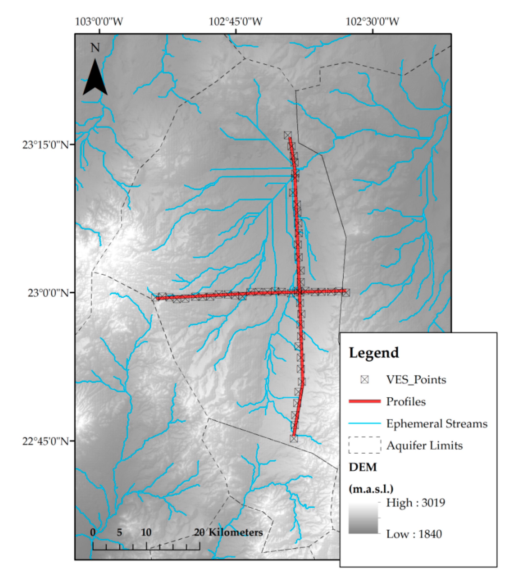
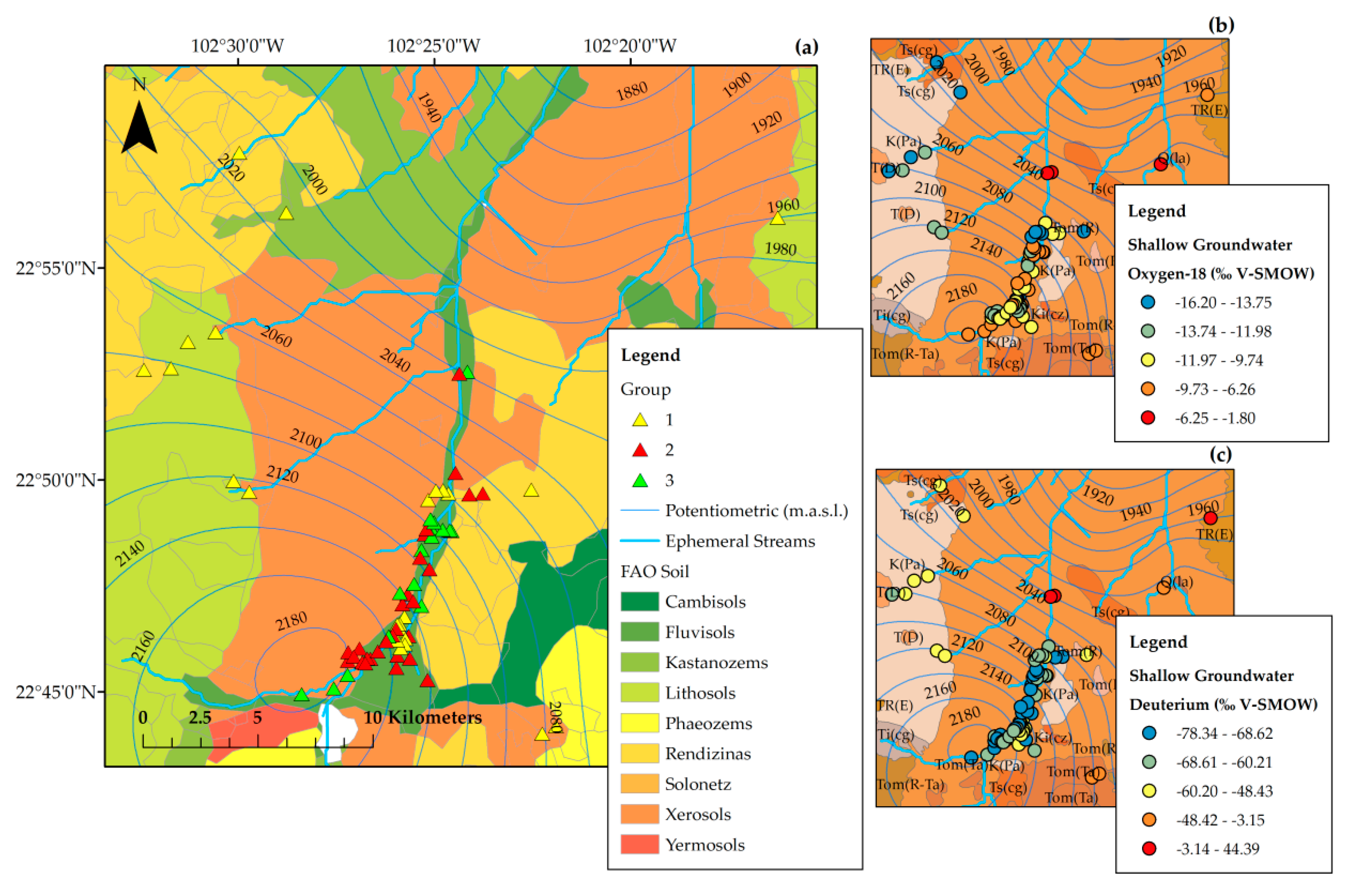
2. Study Site
3. Hydrogeological Setting
4. Methods
4.1. Sampling of Stable Isotopes and Collected Data
4.2. Bivariate Data Analysis
4.3. Geophysical Data Acquisition
5. Results and Discussion
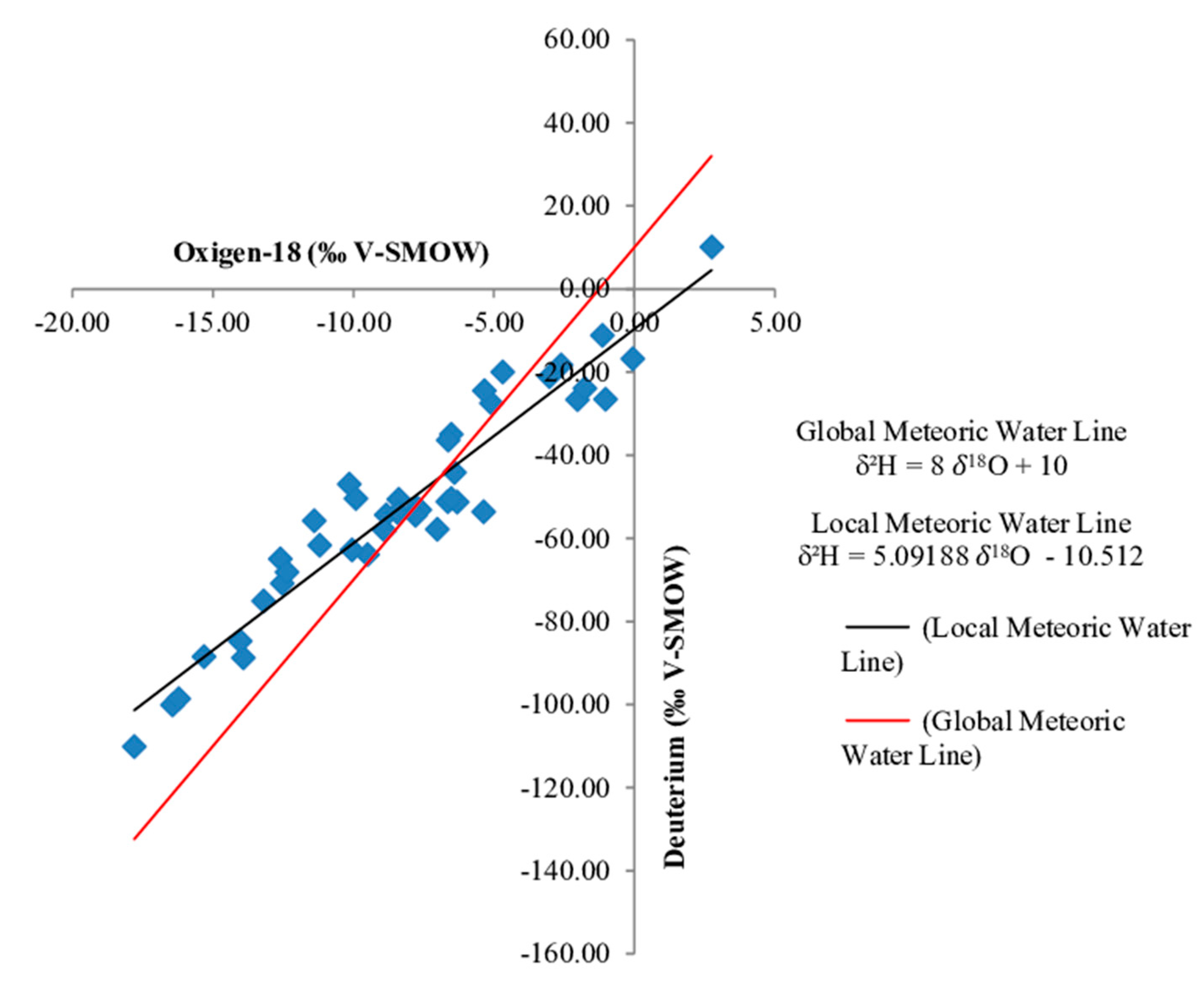
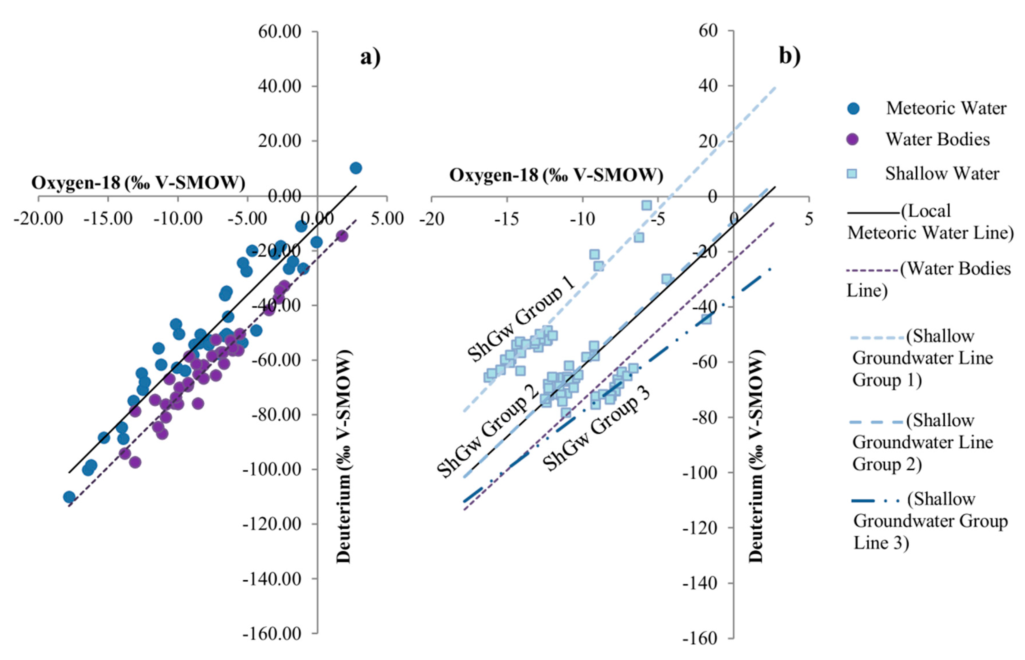
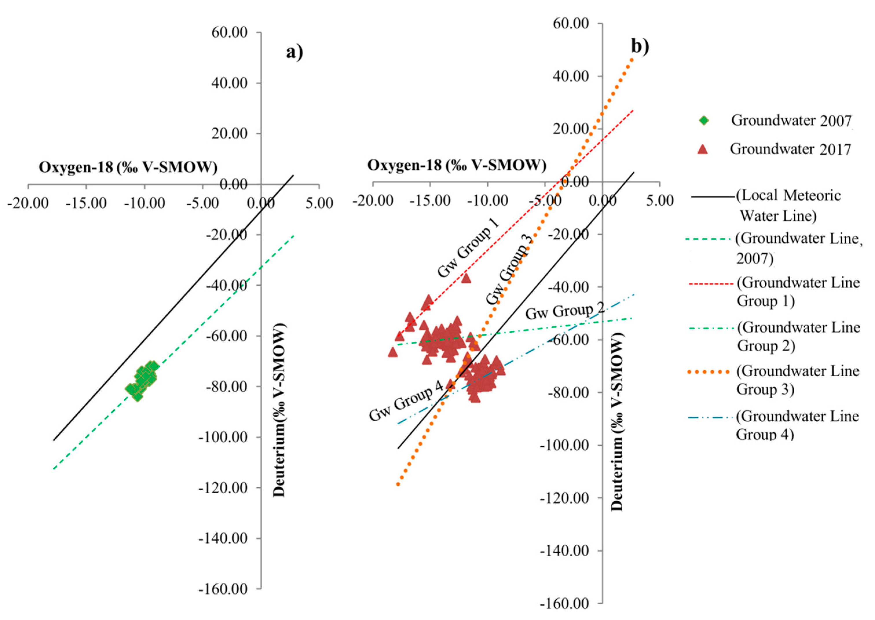
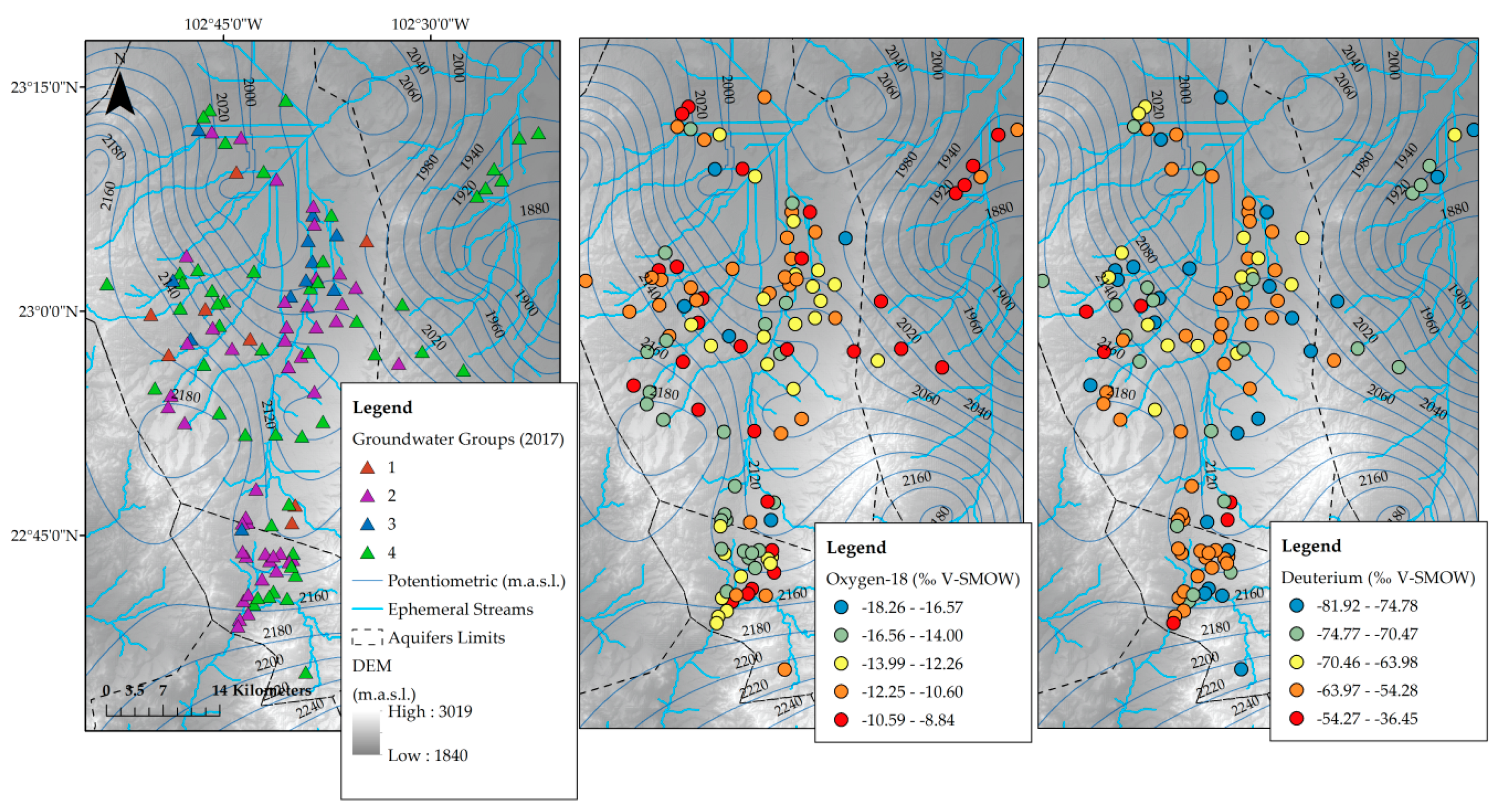
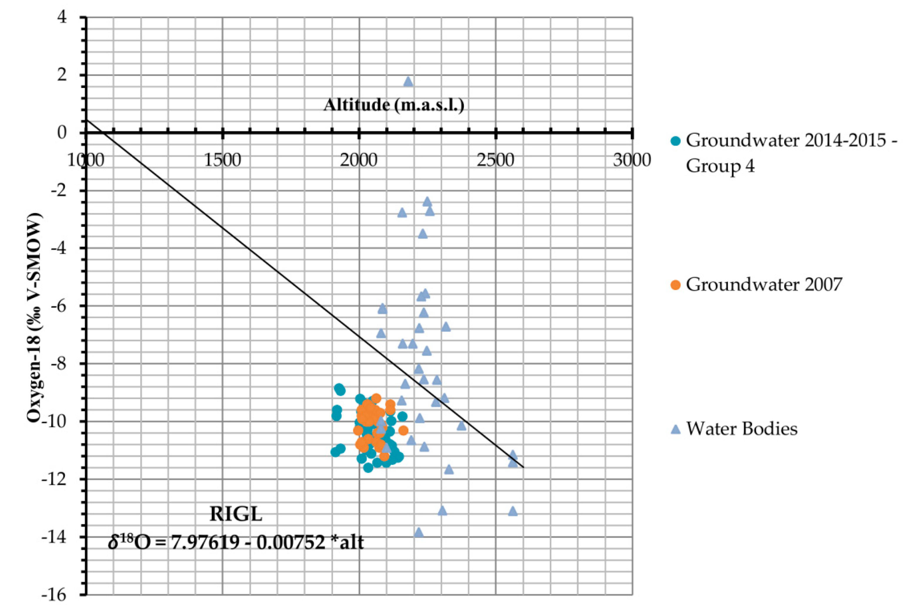
5.1. Isotopic Composition of Water
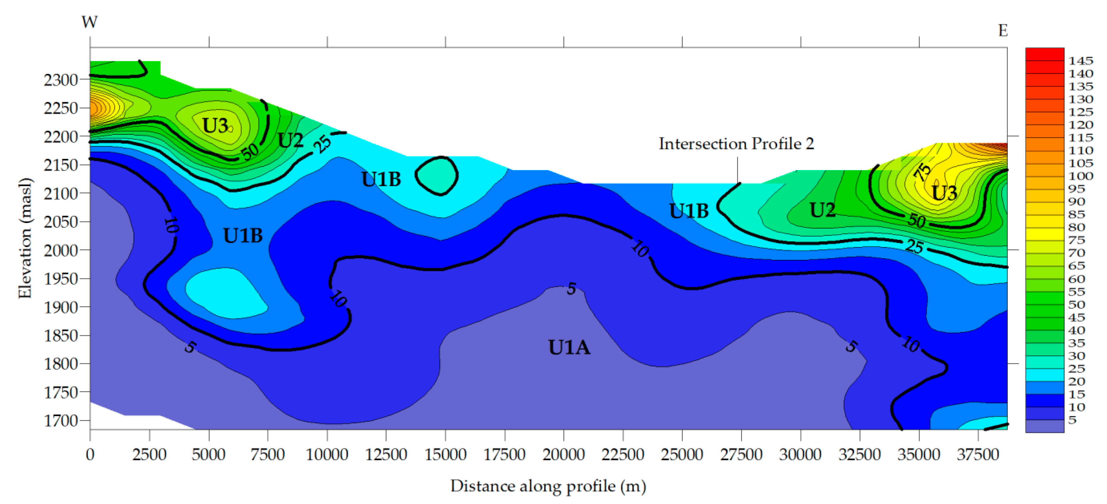
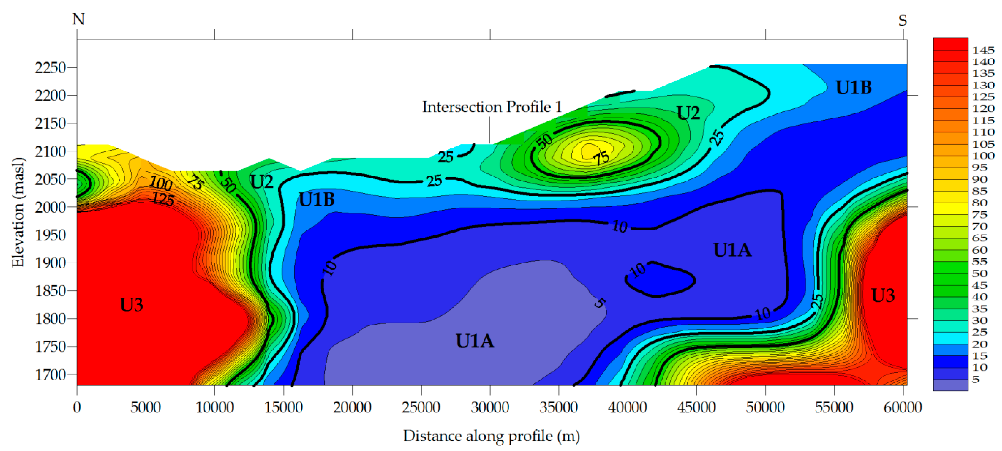
5.2. Geoelectrical Sections
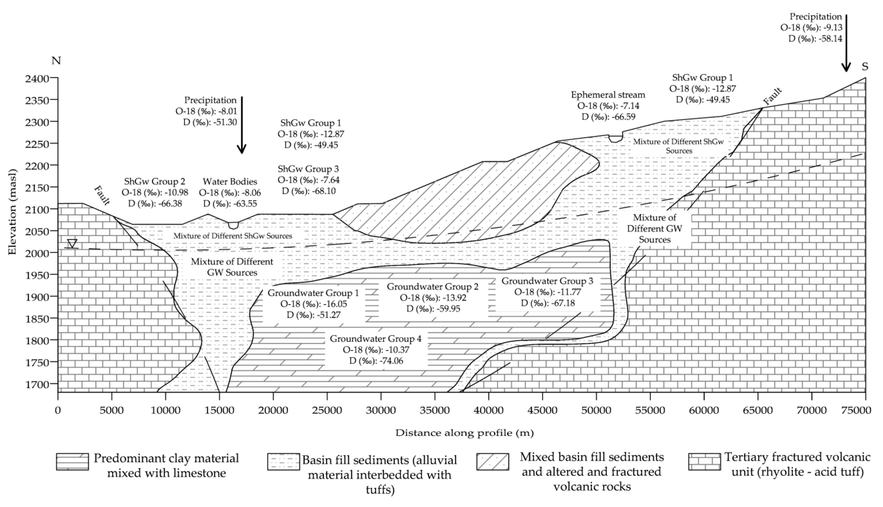
5.3. Conceptual Model
6. Conclusions
Supplementary Materials
Author Contributions
Funding
Acknowledgments
Conflicts of Interest
References
- Kpegli, K.A.R.; Alassane, A.; Trabelsi, R.; Zouari, K.; Boukari, M.; Mama, D.; Dovonon, F.L.; Yoxi, Y.V.; Toro-Espitia, L.E. Geochemical processes in Kandi Basin, Benin, West Africa: A combined hydrochemistry and stable isotopes approach. Quat. Int. 2015, 369, 99–109. [Google Scholar] [CrossRef]
- Shanafield, M.; Cook, P.G. Transmission losses, infiltration and groundwater recharge through ephemeral and intermittent streambeds: A review of applied methods. J. Hydrol. 2014, 511, 518–529. [Google Scholar] [CrossRef]
- Scanlon, B.R.; Keese, K.E.; Flint, A.L.; Flint, L.E.; Gaye, C.B.; Edmunds, W.M.; Simmers, I. Global synthesis of groundwater recharge in semiarid and arid regions. Hydrol. Process. 2006, 20, 3335–3370. [Google Scholar] [CrossRef]
- Ingraham, N.L.; Caldwell, E.A.; Verhagen, B.T. Arid Catchments. In Isotope Tracers in Catchment Hydrology; Elsevier: Amsterdam, The Netherlands, 1998; pp. 435–465. ISBN 978-0-444-81546-0. [Google Scholar]
- Ettayfi, N.; Bouchaou, L.; Michelot, J.L.; Tagma, T.; Warner, N.; Boutaleb, S.; Massault, M.; Lgourna, Z.; Vengosh, A. Geochemical and isotopic (oxygen, hydrogen, carbon, strontium) constraints for the origin, salinity, and residence time of groundwater from a carbonate aquifer in the Western Anti-Atlas Mountains, Morocco. J. Hydrol. 2012, 438–439, 97–111. [Google Scholar] [CrossRef]
- Greenbaum, N. Paleofloods and the Estimation of Long Termn Transmission Losses and Recharge to the Lower Nahal Zin Alluvial Aquifer, Negev Desert, Israel. Anc. Floods Mod. Hazards Princ. Appl. Paleoflood Hydrol. 2002, 5, 311–328. [Google Scholar]
- González-Trinidad, J.; Pacheco-Guerrero, A.; Júnez-Ferreira, H.; Bautista-Capetillo, C.; Hernández-Antonio, A. Identifying Groundwater Recharge Sites through Environmental Stable Isotopes in an Alluvial Aquifer. Water 2017, 9, 569. [Google Scholar] [CrossRef]
- Schoener, G. Quantifying Transmission Losses in a New Mexico Ephemeral Stream: A Losing Proposition. J. Hydrol. Eng. 2017, 22, 05016038. [Google Scholar] [CrossRef]
- McCallum, A.M.; Andersen, M.S.; Acworth, R.I. A New Method for Estimating Recharge to Unconfined Aquifers Using Differential River Gauging. Groundwater 2014, 52, 291–297. [Google Scholar] [CrossRef]
- Goodrich, D.C.; Williams, D.G.; Unkrich, C.L.; Hogan, J.F.; Scott, R.L.; Hultine, K.R.; Pool, D.; Goes, A.L.; Miller, S. Comparison of methods to estimate ephemeral channel recharge, Walnut Gulch, San Pedro River basin, Arizona. In Groundwater Recharge in a Desert Environment. AGU Mon: The Southwestern United States; Wiley: Hoboken, NJ, USA, 2004; pp. 77–99. [Google Scholar]
- Yu, M.C.L.; Cartwright, I.; Braden, J.L.; de Bree, S.T. Examining the spatial and temporal variation of groundwater inflows to a valley-to-floodplain river using 222Rn, geochemistry and river discharge: The Ovens River, southeast Australia. Hydrol. Earth Syst. Sci. 2013, 17, 4907–4924. [Google Scholar] [CrossRef]
- Martinez, J.L.; Raiber, M.; Cox, M.E. Assessment of groundwater–surface water interaction using long-term hydrochemical data and isotope hydrology: Headwaters of the Condamine River, Southeast Queensland, Australia. Sci. Total Environ. 2015, 536, 499–516. [Google Scholar] [CrossRef]
- Scanlon, B.R.; Healy, R.W.; Cook, P.G. Choosing appropriate techniques for quantifying groundwater recharge. Hydrogeol. J. 2002, 10, 18–39. [Google Scholar] [CrossRef]
- Li, Z.; Chen, X.; Liu, W.; Si, B. Determination of groundwater recharge mechanism in the deep loessial unsaturated zone by environmental tracers. Sci. Total Environ. 2017, 586, 827–835. [Google Scholar] [CrossRef] [PubMed]
- Allison, G.B.; Gee, G.W.; Tyler, S.W. Vadose-zone techniques for estimating groundwater recharge in arid and semiarid regions. Soil Sci. Soc. Am. J. 1994, 58, 6–14. [Google Scholar] [CrossRef]
- Liu, Y.; Yamanaka, T.; Zhou, X.; Tian, F.; Ma, W. Combined use of tracer approach and numerical simulation to estimate groundwater recharge in an alluvial aquifer system: A case study of Nasunogahara area, central Japan. J. Hydrol. 2014, 519, 833–847. [Google Scholar] [CrossRef]
- Clark, I.D.; Fritz, P. Environmental Isotopes in Hydrogeology; CRC Press/Lewis Publishers: Boca Raton, FL, USA, 1997; ISBN 978-1-56670-249-2. [Google Scholar]
- Sun, H.; Hu, Z.; Zhang, J.; Wu, W.; Liang, S.; Lu, S.; Liu, H. Determination of hydraulic flow patterns in constructed wetlands using hydrogen and oxygen isotopes. J. Mol. Liq. 2016, 223, 775–780. [Google Scholar] [CrossRef]
- Mogaji, K.A.; Omobude, O.B. Modeling of geoelectric parameters for assessing groundwater potentiality in a multifaceted geologic terrain, Ipinsa Southwest, Nigeria—A GIS-based GODT approach. NRIAG J. Astron. Geophys. 2017, 6, 434–451. [Google Scholar] [CrossRef]
- Younis, A.; Soliman, M.; Moussa, S.; Massoud, U.; ElNabi, S.A.; Attia, M. Integrated geophysical application to investigate groundwater potentiality of the shallow Nubian aquifer at northern Kharga, Western Desert, Egypt. NRIAG J. Astron. Geophys. 2016, 5, 186–197. [Google Scholar] [CrossRef] [Green Version]
- Mohamaden, M.I.I.; Hamouda, A.Z.; Mansour, S. Application of electrical resistivity method for groundwater exploration at the Moghra area, Western Desert, Egypt. Egypt. J. Aquat. Res. 2016, 42, 261–268. [Google Scholar] [CrossRef] [Green Version]
- Wattanasen, K.; Elming, S.-Å. Direct and indirect methods for groundwater investigations: A case-study of MRS and VES in the southern part of Sweden. J. Appl. Geophys. 2008, 66, 104–117. [Google Scholar] [CrossRef]
- Song, L.; Zhu, J.; Yan, Q.; Kang, H. Estimation of groundwater levels with vertical electrical sounding in the semiarid area of South Keerqin sandy aquifer, China. J. Appl. Geophys. 2012, 83, 11–18. [Google Scholar] [CrossRef]
- Lopes, D.D.; Silva, S.M.C.P.; Fernandes, F.; Teixeira, R.S.; Celligoi, A.; Dall’Antônia, L.H. Geophysical technique and groundwater monitoring to detect leachate contamination in the surrounding area of a landfill—Londrina (PR—Brazil). J. Environ. Manag. 2012, 113, 481–487. [Google Scholar] [CrossRef] [PubMed]
- Ruthsatz, A.D.; Sarmiento Flores, A.; Diaz, D.; Reinoso, P.S.; Herrera, C.; Brasse, H. Joint TEM and MT aquifer study in the Atacama Desert, North Chile. J. Appl. Geophys. 2018, 153, 7–16. [Google Scholar] [CrossRef]
- Mohamaden, M.I.I.; Ehab, D. Application of electrical resistivity for groundwater exploration in Wadi Rahaba, Shalateen, Egypt. NRIAG J. Astron. Geophys. 2017, 6, 201–209. [Google Scholar] [CrossRef]
- Helaly, A.S. Assessment of groundwater potentiality using geophysical techniques in Wadi Allaqi basin, Eastern Desert, Egypt—Case study. NRIAG J. Astron. Geophys. 2017, 6, 408–421. [Google Scholar] [CrossRef]
- McLachlan, P.J.; Chambers, J.E.; Uhlemann, S.S.; Binley, A. Geophysical characterisation of the groundwater–surface water interface. Adv. Water Resour. 2017, 109, 302–319. [Google Scholar] [CrossRef]
- Singha, K.; Day-Lewis, F.D.; Johnson, T.; Slater, L.D. Advances in interpretation of subsurface processes with time-lapse electrical imaging. Hydrol. Process. 2015, 29, 1549–1576. [Google Scholar] [CrossRef]
- Binley, A.; Hubbard, S.S.; Huisman, J.A.; Revil, A.; Robinson, D.A.; Singha, K.; Slater, L.D. The emergence of hydrogeophysics for improved understanding of subsurface processes over multiple scales: The Emergence of Hydrogeophysics. Water Resour. Res. 2015, 51, 3837–3866. [Google Scholar] [CrossRef] [PubMed]
- Navarro-SolíS, O.; González-Trinidad, J.; Júnez-Ferreira, H.; Cardona, A.; Bautista-Capetillo, C.F. Integrative methodology for the identification of groundwater flow patterns: Application in a semi-arid region of Mexico. Appl. Ecol. Environ. Res. 2016, 14, 645–666. [Google Scholar] [CrossRef]
- Hernández, J.E.; Gowda, P.H.; Howell, T.A.; Steiner, J.L.; Mojarro, F.; Núñez, E.P.; Avila, J.R. Modeling groundwater levels on the Calera aquifer region in Central Mexico using ModFlow. J. Agric. Sci. Technol. B 2012, 2, 52–61. [Google Scholar]
- Hernández, J.E.; Gowda, P.H.; Howell, T.A.; Steiner, J.L.; Mojarro, F.; Peña Nuñez, E.; Avila, J.R. Groundwater Modeling of the Calera Aquifer Region in Central Mexico; ASCE: Reston, VA, USA, 2011; pp. 1009–1018. [Google Scholar]
- Dailey, D.; Sauck, W.; Sultan, M.; Milewski, A.; Ahmed, M.; Laton, W.R.; Elkadiri, R.; Foster, J.; Schmidt, C.; Al Harbi, T. Geophysical, remote sensing, GIS, and isotopic applications for a better understanding of the structural controls on groundwater flow in the Mojave Desert, California. J. Hydrol. Reg. Stud. 2015, 3, 211–232. [Google Scholar] [CrossRef] [Green Version]
- Navarro-Velasco, J.L. Análisis y Determinaciónde Zonas de Recarga en el Acuífero de Calera, Zacatecas, México; Universidad Autónoma de Zacatecas “Francisco García Salinas”: Zacatecas, México, 2007. [Google Scholar]
- Comisión Nacional del Agua (CONAGUA). Actualización de la Disponibilidad Media Anual de Agua Subterránea, Acuífero (3225) Calera; Diario Oficial de la Federación, Government of Mexico: Mexico City, Mexico, 2015.
- Júnez-Ferreira, H.; González, J.; Reyes, E.; Herrera, G.S. A Geostatistical Methodology to Evaluate the Performance of Groundwater Quality Monitoring Networks Using a Vulnerability Index. Math. Geosci. 2016, 48, 25–44. [Google Scholar] [CrossRef]
- Rosales-Rivera, M.; Díaz-González, L.; Verma, S.P. A new online computer program (BIDASys) for ordinary and uncertainty weighted least-squares linear regressions: case studies from food chemistry. Rev. Mex. Ing. Quím. 2018, 17, 507–522. [Google Scholar] [CrossRef]
- Verma, S.P. Geoquimiometría. Rev. Mex. Cienc. Geológicas 2012, 29, 276–298. [Google Scholar]
- Roy, S.; Tarafdar, S. Archie’s law from a fractal model for porous rocks. Phys. Rev. B 1997, 55, 8038. [Google Scholar] [CrossRef]
- Constable, S.C.; Parker, R.L.; Constable, C.G. Occam’s inversion: A practical algorithm for generating smooth models from electromagnetic sounding data. Geophysics 1987, 52, 289–300. [Google Scholar] [CrossRef]
- Craig, H. Isotopic variations in meteoric waters.pdf. Science 1961, 133, 1702–1703. [Google Scholar] [CrossRef] [PubMed]
- Cartwright, I.; Weaver, T.R.; Cendón, D.I.; Fifield, L.K.; Tweed, S.O.; Petrides, B.; Swane, I. Constraining groundwater flow, residence times, inter-aquifer mixing, and aquifer properties using environmental isotopes in the southeast Murray Basin, Australia. Appl. Geochem. 2012, 27, 1698–1709. [Google Scholar] [CrossRef]
- Liebminger, A.; Haberhauer, G.; Papesch, W.; Heiss, G. Correlation of the isotopic composition in precipitation with local conditions in alpine regions. J. Geophys. Res. 2006, 111, D05104. [Google Scholar] [CrossRef]
- Boronina, A.; Balderer, W.; Renard, P.; Stichler, W. Study of stable isotopes in the Kouris catchment (Cyprus) for the description of the regional groundwater flow. J. Hydrol. 2005, 308, 214–226. [Google Scholar] [CrossRef] [Green Version]
- Luo, X.; Jiao, J.J.; Wang, X.; Liu, K.; Lian, E.; Yang, S. Groundwater discharge and hydrologic partition of the lakes in desert environment: Insights from stable 18O/2H and radium isotopes. J. Hydrol. 2017, 546, 189–203. [Google Scholar] [CrossRef]
- Karroum, M.; Elgettafi, M.; Elmandour, A.; Wilske, C.; Himi, M.; Casas, A. Geochemical processes controlling groundwater quality under semi arid environment: A case study in central Morocco. Sci. Total Environ. 2017, 609, 1140–1151. [Google Scholar] [CrossRef] [PubMed]
- Herczeg, A.L.; Barnes, C.J.; Macumber, P.G.; Olley, J.M. A stable isotope investigation of groundwater-surface water interactions at Lake Tyrrell, Victoria, Australia. Chem. Geol. 1992, 96, 19–32. [Google Scholar] [CrossRef]
- Goebel, T.S.; Lascano, R.J.; Paxton, P.R.; Mahan, J.R. Rainwater use by irrigated cotton measured with stable isotopes of water. Agric. Water Manag. 2015, 158, 17–25. [Google Scholar] [CrossRef]
- Keesari, T.; Sharma, D.A.; Rishi, M.S.; Pant, D.; Mohokar, H.V.; Jaryal, A.K.; Sinha, U.K. Isotope investigation on groundwater recharge and dynamics in shallow and deep alluvial aquifers of southwest Punjab. Appl. Radiat. Isot. 2017, 129, 163–170. [Google Scholar] [CrossRef] [PubMed]
- Lu, Y.; Tang, C.; Chen, J.; Song, X.; Li, F.; Sakura, Y. Spatial characteristics of water quality, stable isotopes and tritium associated with groundwater flow in the Hutuo River alluvial fan plain of the North China Plain. Hydrogeol. J. 2008, 16, 1003–1015. [Google Scholar] [CrossRef] [Green Version]
- Gaye, C.B.; Edmunds, W.M. Groundwater recharge estimation using chloride, stable isotopes and tritium profiles in the sands of northwestern Senegal. Environ. Geol. 1996, 27, 246–251. [Google Scholar] [CrossRef] [Green Version]
- Tan, H.; Liu, Z.; Rao, W.; Wei, H.; Zhang, Y.; Jin, B. Stable isotopes of soil water: Implications for soil water and shallow groundwater recharge in hill and gully regions of the Loess Plateau, China. Agric. Ecosyst. Environ. 2017, 243, 1–9. [Google Scholar] [CrossRef]
- Souza, R.; Souza, E.; Netto, A.M.; de Almeida, A.Q.; Júnior, G.B.; Silva, J.R.I.; de Sousa Lima, J.R.; Antonino, A.C.D. Assessment of the physical quality of a Fluvisol in the Brazilian semiarid region. Geoderma Reg. 2017, 10, 175–182. [Google Scholar] [CrossRef]
- Abadi Berhe, B.; Erdem Dokuz, U.; Çelik, M. Assessment of hydrogeochemistry and environmental isotopes of surface and groundwaters in the Kütahya Plain, Turkey. J. Afr. Earth Sci. 2017, 134, 230–240. [Google Scholar] [CrossRef]
- Ako, A.A.; Shimada, J.; Hosono, T.; Ichiyanagi, K.; Nkeng, G.E.; Eyong, G.E.T.; Roger, N.N. Hydrogeochemical and isotopic characteristics of groundwater in Mbanga, Njombe and Penja (Banana Plain)—Cameroon. J. Afr. Earth Sci. 2012, 75, 25–36. [Google Scholar] [CrossRef]
- Bouragba, L.; Mudry, J.; Bouchaou, L.; Hsissou, Y.; Krimissa, M.; Tagma, T.; Michelot, J.L. Isotopes and groundwater management strategies under semi-arid area: Case of the Souss upstream basin (Morocco). Appl. Radiat. Isot. 2011, 69, 1084–1093. [Google Scholar] [CrossRef] [PubMed]
- Dogramaci, S.; Skrzypek, G.; Dodson, W.; Grierson, P.F. Stable isotope and hydrochemical evolution of groundwater in the semi-arid Hamersley Basin of subtropical northwest Australia. J. Hydrol. 2012, 475, 281–293. [Google Scholar] [CrossRef]
- Carucci, V.; Petitta, M.; Aravena, R. Interaction between shallow and deep aquifers in the Tivoli Plain (Central Italy) enhanced by groundwater extraction: A multi-isotope approach and geochemical modeling. Appl. Geochem. 2012, 27, 266–280. [Google Scholar] [CrossRef]
- Petitta, M.; Primavera, P.; Tuccimei, P.; Aravena, R. Interaction between deep and shallow groundwater systems in areas affected by Quaternary tectonics (Central Italy): A geochemical and isotope approach. Environ. Earth Sci. 2011, 63, 11–30. [Google Scholar] [CrossRef]
- Addai, M.O.; Yidana, S.M.; Chegbeleh, L.-P.; Adomako, D.; Banoeng-Yakubo, B. Groundwater recharge processes in the Nasia sub-catchment of the White Volta Basin: Analysis of porewater characteristics in the unsaturated zone. J. Afr. Earth Sci. 2016, 122, 4–14. [Google Scholar] [CrossRef]
- Ahmed, A.; Clark, I. Groundwater flow and geochemical evolution in the Central Flinders Ranges, South Australia. Sci. Total Environ. 2016, 572, 837–851. [Google Scholar] [CrossRef]
- Bestland, E.; George, A.; Green, G.; Olifent, V.; Mackay, D.; Whalen, M. Groundwater dependent pools in seasonal and permanent streams in the Clare Valley of South Australia. J. Hydrol. Reg. Stud. 2017, 9, 216–235. [Google Scholar] [CrossRef] [Green Version]
- Gonfiantini, R.; Roche, M.-A.; Olivry, J.-C.; Fontes, J.-C.; Zuppi, G.M. The altitude effect on the isotopic composition of tropical rains. Chem. Geol. 2001, 181, 147–167. [Google Scholar] [CrossRef]
- Dansgaard, W. Stable isotopes in precipitation. Tellus 1964, 4, 438–467. [Google Scholar]
- N’da, A.B.; Bouchaou, L.; Reichert, B.; Hanich, L.; Ait Brahim, Y.; Chehbouni, A.; Beraaouz, E.H.; Michelot, J.-L. Isotopic signatures for the assessment of snow water resources in the Moroccan high Atlas mountains: Contribution to surface and groundwater recharge. Environ. Earth Sci. 2016, 75, 755. [Google Scholar] [CrossRef]
- Paternoster, M.; Liotta, M.; Favara, R. Stable isotope ratios in meteoric recharge and groundwater at Mt. Vulture volcano, southern Italy. J. Hydrol. 2008, 348, 87–97. [Google Scholar] [CrossRef]


| δ2H (‰) | δ18O (‰) | |||||||||
|---|---|---|---|---|---|---|---|---|---|---|
| Sample Source | Year | No. of Samples | Average | Max | Min | Std. Dev. | Average | Max | Min | Std. Dev. |
| Precipitation | 2016–2018 | 43 | −51.34 | 10.11 | −110.20 | 25.81 | −8.10 | 2.74 | −17.80 | 4.78 |
| Water Bodies | 2018 | 37 | −63.55 | −14.64 | −97.32 | 17.17 | −8.06 | 1.78 | −13.82 | 3.32 |
| Stream Runoff | 2018 | 3 | −66.59 | −66.26 | −66.91 | 0.33 | −7.14 | −7.07 | −7.19 | 0.06 |
| Shallow Groundwater | 2017 | 69 | −60.65 | −3.15 | −78.34 | 14.36 | −10.89 | −1.80 | −16.20 | 2.85 |
| Groundwater [7] | 2014–2015 | 115 | −66.05 | −36.45 | −81.92 | 8.62 | −12.35 | −8.84 | −18.26 | 2.13 |
| Groundwater [35] | 2007 | 35 | −77.57 | −72.00 | −84.00 | 3.00 | −10.05 | −9.20 | −11.20 | 0.52 |
| Sample Source | Groups | Disc. Val. (OLR) | OLR | R | R2 |
|---|---|---|---|---|---|
| Precipitation | 1 | 0 | δ2H = 5.0918(±0.7149) δ18O − 10.5123(±6.6357) | 0.9488 | 0.9003 |
| Water Bodies | 1 | 9 | δ2H = 5.0911(±0.3999) δ18O − 22.9363(±3.2283) | 0.9898 | 0.9797 |
| Shallow Groundwater | 1 | 0 | δ2H = 5.6985(±0.8418) δ18O + 23.8678(±11.0597) | 0.9696 | 0.9401 |
| 2 | 1 | δ2H = 5.2056(±1.1003) δ18O − 8.7896(±12.2007) | 0.9351 | 0.8743 | |
| 3 | 0 | δ2H = 4.1607(±0.8470) δ18O − 36.3241(±6.6212) | 0.9688 | 0.9386 | |
| Groundwater [7] | 1 | 0 | δ2H = 4.1795(±1.9141) δ18O + 15.8187(±30.9319) | 0.9571 | 0.9161 |
| 2 | 4 | δ2H = 0.4915(±1.1993) δ18O − 53.0963(±16.7044) | 0.1704 | 0.029 | |
| 3 | 0 | δ2H = 7.9114(±4.5891) δ18O + 25.9673(±51.0982) | 0.8816 | 0.7772 | |
| 4 | 0 | δ2H = 2.3849(±1.6652) δ18O − 49.3238(±17.3052) | 0.4892 | 0.2393 | |
| Groundwater [35] | 1 | 8 | δ2H = 5.0829(±1.0577) δ18O − 26.7229(±10.6285) | 0.9369 | 0.8777 |
| Sample Source | Groups | Disc. Val. (UWLR) | UWLR | R | R2 |
|---|---|---|---|---|---|
| Precipitation | 1 | 0 | δ2H = 5.0918(±0.2647) δ18O − 10.5123(±2.4577) | 0.9488 | 0.9003 |
| Water Bodies | 1 | 5 | δ2H = 5.0795(±0.1900) δ18O − 22.9634(±1.5722) | 0.9797 | 0.9597 |
| Shallow Groundwater | 1 | 0 | δ2H = 5.6985(±0.2999) δ18O + 23.8678(±3.9395) | 0.9696 | 0.9401 |
| 2 | 1 | δ2H = 5.2056(±0.3947) δ18O − 8.7896(±4.3770) | 0.9351 | 0.8743 | |
| 3 | 0 | δ2H = 4.1607(±0.2845) δ18O − 36.3241(±2.2242) | 0.9688 | 0.9386 | |
| Groundwater [7] | 1 | 0 | δ2H = 4.1795(±0.6163) δ18O +15.8187(±8.3430) | 0.9571 | 0.9161 |
| 2 | 4 | δ2H = 0.4915(±0.4440) δ18O − 53.0963(±6.1841) | 0.1704 | 0.029 | |
| 3 | 0 | δ2H = 7.9114(±1.4122) δ18O + 25.9673(±16.6466) | 0.8816 | 0.7772 | |
| 4 | 0 | δ2H = 2.3849(±0.6203) δ18O − 49.3238(±6.4462) | 0.4892 | 0.2393 | |
| Groundwater [35] | 1 | 4 | δ2H = 4.4808(±0.4320) δ18O − 32.7572(±4.33981) | 0.8875 | 0.7877 |
| Sample Source | Year | Group | n | Average | Max | Min | Std Dev |
|---|---|---|---|---|---|---|---|
| Precipitation | 2014–2018 | 1 | 43 | 13.42 | 35.80 | −18.31 | 15.62 |
| Water Bodies | 2018 | 1 | 37 | 0.96 | 25.83 | −28.88 | 11.18 |
| Stream Runoff | 1 | 3 | −9.49 | −9.06 | −10.35 | 0.74 | |
| Shallow Groundwater | 2017 | 1 | 25 | 53.48 | 64.09 | 35.18 | 7.36 |
| 2 | 28 | 21.49 | 30.72 | 5.63 | 5.73 | ||
| 3 | 16 | −7.00 | 0.64 | −30.00 | 6.84 | ||
| Groundwater [7] | 2014–2015 | 1 | 8 | 77.15 | 82.94 | 58.42 | 8.01 |
| 2 | 47 | 51.42 | 69.89 | 36.93 | 7.55 | ||
| 3 | 11 | 27.01 | 33.01 | 23.70 | 2.63 | ||
| 4 | 49 | 8.91 | 19.23 | −0.85 | 4.80 | ||
| Groundwater [35] | 2007 | 1 | 35 | 2.82 | 8.60 | −1.80 | 2.44 |
| Unit | Resistivity (Ωm) | Geological Correlation |
|---|---|---|
| 1A | <10 | Predominant clay material mixed with limestone |
| 1B | 10–25 | Basin fill sediments (alluvial material interbedded with tuffs) |
| 2 | 25–50 | Mixture basin fill sediments and altered and fractured volcanic rocks |
| 3 | >50 | Tertiary fractured volcanic unit which is represented by rhyolite |
© 2019 by the authors. Licensee MDPI, Basel, Switzerland. This article is an open access article distributed under the terms and conditions of the Creative Commons Attribution (CC BY) license (http://creativecommons.org/licenses/by/4.0/).
Share and Cite
Anuard, P.-G.; Julián, G.-T.; Hugo, J.-F.; Carlos, B.-C.; Arturo, H.-A.; Edith, O.-T.; Claudia, Á.-S. Integration of Isotopic (2H and 18O) and Geophysical Applications to Define a Groundwater Conceptual Model in Semiarid Regions. Water 2019, 11, 488. https://doi.org/10.3390/w11030488
Anuard P-G, Julián G-T, Hugo J-F, Carlos B-C, Arturo H-A, Edith O-T, Claudia Á-S. Integration of Isotopic (2H and 18O) and Geophysical Applications to Define a Groundwater Conceptual Model in Semiarid Regions. Water. 2019; 11(3):488. https://doi.org/10.3390/w11030488
Chicago/Turabian StyleAnuard, Pacheco-Guerrero, González-Trinidad Julián, Júnez-Ferreira Hugo, Bautista-Capetillo Carlos, Hernández-Antonio Arturo, Olmos-Trujillo Edith, and Ávila-Sandoval Claudia. 2019. "Integration of Isotopic (2H and 18O) and Geophysical Applications to Define a Groundwater Conceptual Model in Semiarid Regions" Water 11, no. 3: 488. https://doi.org/10.3390/w11030488