Article

Stochastic Method for Evaluating Removal, Fate and Associated Uncertainties of Micropollutants in a Stormwater Biofilter at an Annual Scale

1
LEESU, UMR MA 102, École des Ponts, AgroParisTech, UPEC, UPE, Champs-sur-Marne, 6-8 avenue Blaise Pascal, Cité Descartes, 77455 Marne-la-Vallée CEDEX 2, France
2
CEREMA, 12 Rue Léon Teisserenc de Bort, 78190 Trappes, France
3
IFSTTAR, Laboratoire Eau et Environnement- route de Bouaye CS4, 44344 Bouguenais CEDEX, France
*
Authors to whom correspondence should be addressed.
Water 2019, 11(3), 487; https://doi.org/10.3390/w11030487
Submission received: 18 January 2019 / Revised: 20 February 2019 / Accepted: 26 February 2019 / Published: 9 March 2019

Abstract

:
A stochastic method for evaluating the in situ mass balance of micropollutants in a stormwater biofilter, accounting for inlet and outlet loads and the evolution of pollutant mass in the filter media (ΔMsoil) at an annual scale, is proposed. In the field context, this type of calculation presents a number of methodological challenges, associated with estimating water quality for unsampled rain events, reconstituting missing or invalidated flow data and accounting for significant uncertainties associated with these estimations and experimental measurements. The method is applied to a biofiltration swale treating road runoff for two trace metals, Cu and Zn and six organic micropollutants: pyrene (Pyr), phenanthrene (Phen), bisphenol-A (BPA), octylphenol (OP), nonylphenol (NP) and bis(2-ethylhexyl) phthalate (DEHP). Pollutant loads were reduced by 27–72%. While organic micropollutants are likely to be lost to degradation or volatilization processes in such systems, dissipation could not be demonstrated for any of the organic micropollutants studied due to emissions from construction materials (case of BPA, OP, NP and DEHP) or high uncertainties in ΔMsoil (case of Pyr and Phen). The necessary conditions for establishing an in situ mass balance demonstrating dissipation, which include acquisition of data associated with all terms over a period long enough that uncertainty propagation is limited and the absence of additional sources of pollutants in the field, are discussed.

1. Introduction

In order to minimize the effects of urbanization on the water cycle and aquatic environments, new paradigms for urban stormwater management have emerged and gained in popularity. Known under the terms low impact development (LID), sustainable drainage systems (SuDS) or water sensitive urban design (WSUD), these approaches advocate managing urban runoff close to the source, often through soil-based, vegetated devices, designed to improve water quality and meet hydrologic objectives while contributing to the urban landscape and biodiversity [1]. The European Water Framework Directive imposes environmental quality standards for a number of priority pollutants, including trace metals and organic micropollutants [2]; within this context, managing priority pollutants present in urban runoff has become a major objective for urban stormwater infrastructures.
One technique specifically designed for pollution control, referred to as biofiltration or bioretention, consists of a vegetated depression that receives and stores runoff water, which then filters through a filter media or engineered soil, before being collected by an underdrain or exfiltrated to the surrounding soil [3,4]. In these devices, pollutants are expected to undergo various processes including sedimentation, physical filtration, sorption, biodegradation, volatilization and plant uptake [5].
The effectiveness of a system of this type at managing pollution may be considered on two levels. The first is its ability to reduce pollutant loads at the outlets of the system; this may be achieved by separating pollutants from infiltrating water, often via filtration and/or sorption or by retaining water containing pollutants in the soil pores. This type of performance, which has been evaluated in field-scale biofiltration systems for a variety of pollutants including total suspended solids (TSS), nutrients, trace metals and polycyclic aromatic hydrocarbons (PAHs) [6,7,8,9,10], protects water bodies by limiting the mass of pollutants transported to them. Its evaluation requires knowledge of both concentrations and flows entering and exiting a system over a given period. To fully characterize the performance of such a system in terms of pollutant load reduction, it should be evaluated over a period of at least a year, in order to account for inter-event and seasonal variability in both inlet loads and system performance [10,11,12].
Some pollutants, such as organic micropollutants, may be dissipated through natural processes, such as biodegradation, volatilization and photodegradation [5,13]. A system’s performance may also be evaluated in terms of its ability to dissipate these pollutants, thereby minimizing their overall presence in the environment and their accumulation in the soil, a potentially adverse effect of pollutant retention, which may be associated with toxicity to the ecosystem of the biofilter, compromising its long-term viability, or, if the site is accessible to the public, a risk to human health [13]. The evaluation of this type of performance requires information about the mass of a pollutant intercepted by the biofilter and evolution of the mass stored in its soil over time. We note that no dissipation is expected for conservative pollutants, such as trace metals.
The potential for dissipation in biofiltration systems has been demonstrated at the laboratory scale for oil and grease [14], naphthalene [15] and at the mesocosm scale for PAHs [16]. These controlled approaches allow for the quantification of mass proportions attributed to various fate processes. However, the behaviour in these experiments may not always be representative of that in field systems. For one thing, the complex environment of a field system is difficult to reproduce under controlled conditions. In addition, both the speciation of the laboratory-grade chemicals and the high concentrations applied tend to be quite different from those observed in real runoff, which may lead to higher bioavailability than in the field. Field approaches have also demonstrated the occurrence of dissipation by comparing measured soil concentrations to simple load calculations from the literature [17] or by comparing pollutants distributions observed in soil to those observed in runoff [7].
The establishment of an in situ mass balance for a stormwater biofilter, accounting for inlet and outlet loads, as well as pollutant accumulation in the filter media, would allow for an integrated evaluation of both types of pollutant control performance over a given period. While many studies have studied the mass balance of pollutants in stormwater biofilters to characterize load reduction at an event scale [6,7,9,18], to the author’s knowledge, no previous studies have made a rigorous attempt to establish such a balance over a longer period in order to characterize both the retention and the fate of organic micropollutants. Indeed, such a task involves a number of methodological challenges. For one thing, due to the labour-intensive nature of water quality sampling and analysis, it is not possible to sample all rainfall over a long period; it is therefore necessary to estimate water quality for unsampled events in the studied period. In addition, a number of technical dysfunctions may result in missing or invalid data in continuous measurement series of rainfall, flow or water quality parameters [19,20]; in this case, medium- or long-term load estimations require a reconstitution of this data. These reconstitutions, as well the measurements, sampling and analyses of any stormwater monitoring campaign, entail uncertainties, which must be accounted for in order to draw pertinent conclusions [21]. The objective of the present work is to present and test a stochastic method for evaluating such a mass balance, accounting for its uncertainties. The method is applied to a selection of micropollutants with varying properties, which are typical of road runoff.

2. Materials and Methods

2.1. Field Methods

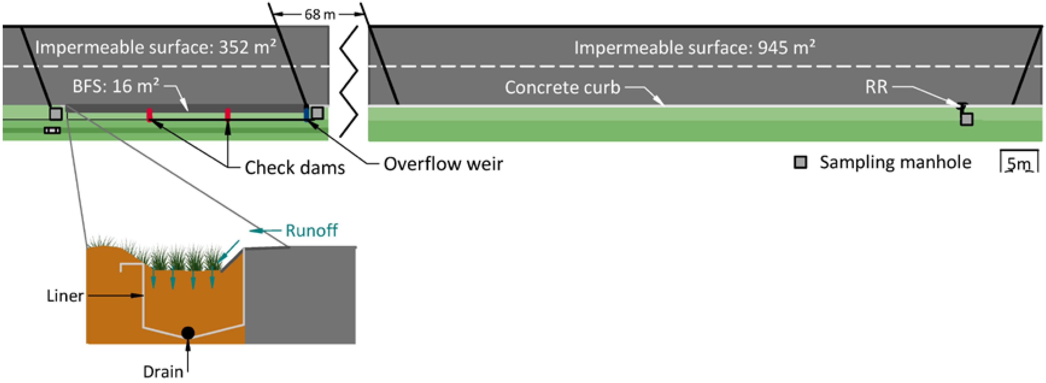
2.1.1. Site Description

The study site includes a biofiltration swale (BFS), which drains water from the RD 212, a highway with a daily traffic of 11,000 vehicles/day, located in Compans, France in the Paris region. The BFS is separated from the road surface by a galvanized steel safety barrier and a thin strip of sloped asphalt, added at the time of construction to guide runoff into the swale. The characteristics of this system, which began operation on 18 March 2016, are described in Table 1. It is lined and water was collected from a drain beneath the filter media at a depth of 50 cm. Its filter media was prepared by mixing 40% (by volume) silt loam topsoil with 60% 0–4 mm limestone sand using a rototiller. The mixed filter media includes a significant proportion of grains greater than 2 mm (27 ± 4.5% relative standard deviation); the fraction below 2 mm has a sandy loam texture. The media was found to be less dense at the surface (1.7 kg/L in the first 5 cm) than at greater depths (1.9 kg/L), with a deviation of as much as ±20% among measurements at the same depth. The system was designed to treat small, frequent rain events. As the terrain had a 1.3% slope parallel to the road, the BFS was divided into three sections with concrete check dams (installed in June 2016, after 3 months of operation) to increase surface storage volume, yielding an average ponding depth of 17 cm.
Untreated road runoff (RR), considered to be representative of the quality of water entering the BFS, was collected from a reference catchment at a nearby section of the same road (Figure 1).

2.1.2. Continuous Measurements

Rainfall was measured on site with a tipping bucket rain gauge. RR and BFS drain flows were continuously measured (from November 2015–April 2017 for RR and from April 2016–April 2017 for BFS) using tipping bucket flow meters (17 L bucket volume at RR and 1 L volume at BFS). The BFS overflow was measured using a V-notch weir beginning in October 2016. Rainfall measurements were validated by comparison with external rain gauges from the Paris region and comparison with flow measurements. Flow measurements were compared with rainfall for validation and tipping bucket volumes were verified in situ.
RR was also equipped with a multiparameter probe, which continuously measured both electrical conductivity and turbidity in the untreated runoff. Flow-weighted mean turbidity measurements for sampled events were cross-validated with laboratory-measured turbidity and total suspended solids (TSS) measurements for sampled events. In addition, potentially faulty turbidity measurements were identified using several criteria: (minimal turbidity < 0 Formazin Nephelometric Units (FNU), maximal turbidity > 800 FNU, changes in turbidity greater than ± 200 FNU/min, variation of turbidity over an event of less than 200 FNU over a full event or event mean turbidity less than 70 FNU) [22]. For events containing at least one of these criteria, turbidity was visualized along with the hydrograph before a decision as to its validation was made.

2.1.3. Water Sampling and Pre-Treatment

Water sampling is detailed elsewhere [23]. Briefly, water was collected in proportion to flow volume in order to estimate event mean concentrations. Sampling began in February 2016 for RR and in May 2016 for BFS; a total of 14 and 15 events were sampled, respectively. 11 of these events were sampled simultaneously at both locations, while the remaining events were sampled at only one point due to different starting dates and technical difficulties. Sampling covered all four seasons and a variety of hydrologic conditions. Figure A1 in Appendix A presents a timeline of sampled events along with daily rainfall.
Water samples were collected within 24 h of each rain event and sent to partner laboratories within 24 h of collection where they are immediately filtered. Water was analysed for a large number of water quality parameters and micropollutants [23], which were analysed in the particulate and dissolved phases. The present work focuses on a subset of these parameters, chosen to represent the pollutants from different families and with varying properties: total suspended solids (TSS), organic carbon (OC), two trace metals (Cu and Zn), two PAHs (pyrene–Pyr and phenanthrene–Phen), bisphenol A (BPA), two alkylphenols (octylphenol–OP and nonylphenol–NP) and one phthalate (bis(2-ethylhexyl) phthalate–DEHP).

2.1.4. Soil Sampling and Preparation

An initial sample of filter media (soil) was taken from the previously mixed filter media before its installation in the BFS in March 2016.
The filter media in the BFS was sampled in April 2017 according to the method developed by Tedoldi et al. [24], which relies on a sampling procedure in two phases. First, the surface of the BFS was sampled using an identical high-resolution grid in each section of the BFS (Figure 2a); each sample was dried, sieved to 2 mm, homogenized and analysed for Cu, Zn and Pb using portable X-ray fluorescence spectrometry. Resulting soil concentrations were interpolated to establish a cartography of trace metal surface contamination, which was then used to choose 2–3 zones of similar contamination in each section. In each zone, 2–4 cores were collected (Figure 2b) using a stainless steel gouge auger (3 cm inner diameter), which was cleaned and rinsed twice with ultrapure water between samples. Each core was divided into three segments: 0–5 cm, 5–15 cm and 15–50 cm. Samples from each depth and each zone were combined to form a composite sample.
Each composite sample was quartered and separated into subsamples, which were stored and prepared according to the intended analysis. For trace metal analysis, samples were stored in plastic bags, sieved to 2 mm and acid digested according to the standard NF X31-147 (total digestion). Samples analysed for organic micropollutants were stored in grilled, amber glass jars, immediately frozen upon arrival at the laboratory, then freeze-dried, ground and sieved to 2 mm before extraction and analysis.
The initial sample and the soil cores were analysed for organic carbon and the same micropollutants as were analysed in water [23]; among these, the present work focuses on OC, Cu, Zn, Pyr, Phen, BPA, OP and NP.

2.1.5. Analytical Methods

The analytical methods, limits of quantification (LoQ) and analytical uncertainties for the pollutants detailed in the present article are summarized in Table 2.

2.2. Mass Balance and Uncertainty Calculations

A mass balance was evaluated for the selected pollutants in the BFS according to Equation (1) over a period of the first 13 months of operation (18 March 2016 through 18 April 2017). Available experimental data were combined with modelling or interpolation approaches in order to calculate each term, the details of which are described in the following paragraphs. In order to account for uncertainty, a Monte Carlo approach was used, wherein uncertain values used in the calculation of these terms were varied stochastically (see Appendix B for lists of all stochastically varied parameters and distributions used). All calculations were repeated 10,000 times.
M s o i l , f i n a l M s o i l , i n i t i a l = M i n , R R M o u t , d r a i n M o u t , o v e r + Δ M
where M s o i l , i n i t i a l is the mass of pollutant present in the soil at the beginning of the period, M s o i l , f i n a l is the mass of pollutant in the soil at the end of the period, M i n , R R is the pollutant load from road runoff, M o u t , d r a i n is the pollutant load in the outflow from the drain, M o u t , o v e r is the pollutant load in the system overflow and Δ M is the difference in the characterized masses–a positive Δ M indicates that some dissipation of a pollutant has occurred and a negative Δ M corresponds to a pollutant for which an additional source is present.
It is to be noted that this formulation of the mass balance assumes that runoff water is the only pertinent source of pollution, neglecting other potential sources of pollution, including direct atmospheric deposition. The validity of this assumption will be evaluated in the discussion section.
Terms of the mass balance were used to calculate the efficiency of the system at intercepting pollutant loads (Eint, Equation (2)) and to compare accumulation in the soil (ΔMsoil = Msoil,finalMsoil,initial) with the intercepted mass (Mintercepted = Min,RRMout,drainMout,over).
E i n t = 1 M o u t , d r a i n + M o u t , o v e r M i n , R R
where Eint is the percent mass of pollutant retained by the system, M o u t , d r a i n is pollutant load in the outflow from the drain, M o u t , o v e r is the pollutant load in the system overflow and M i n , R R is the pollutant load from road runoff.

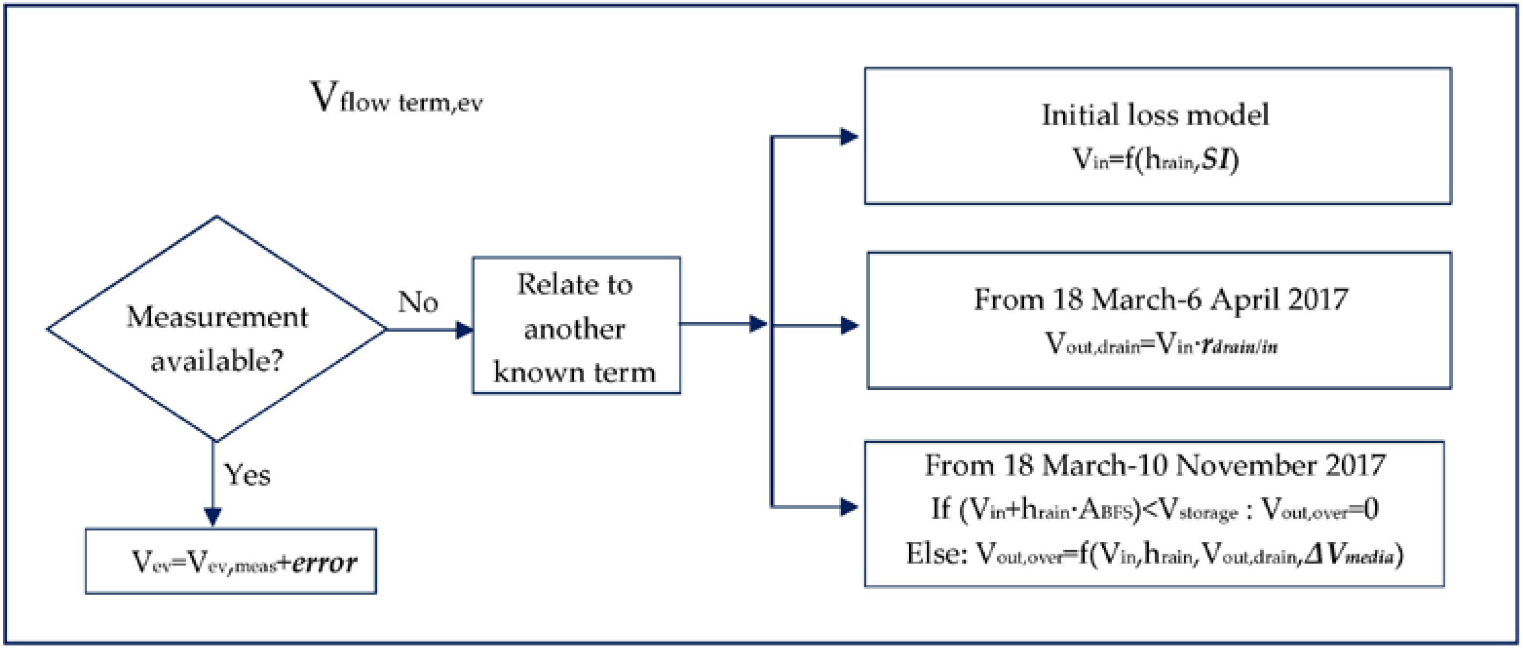
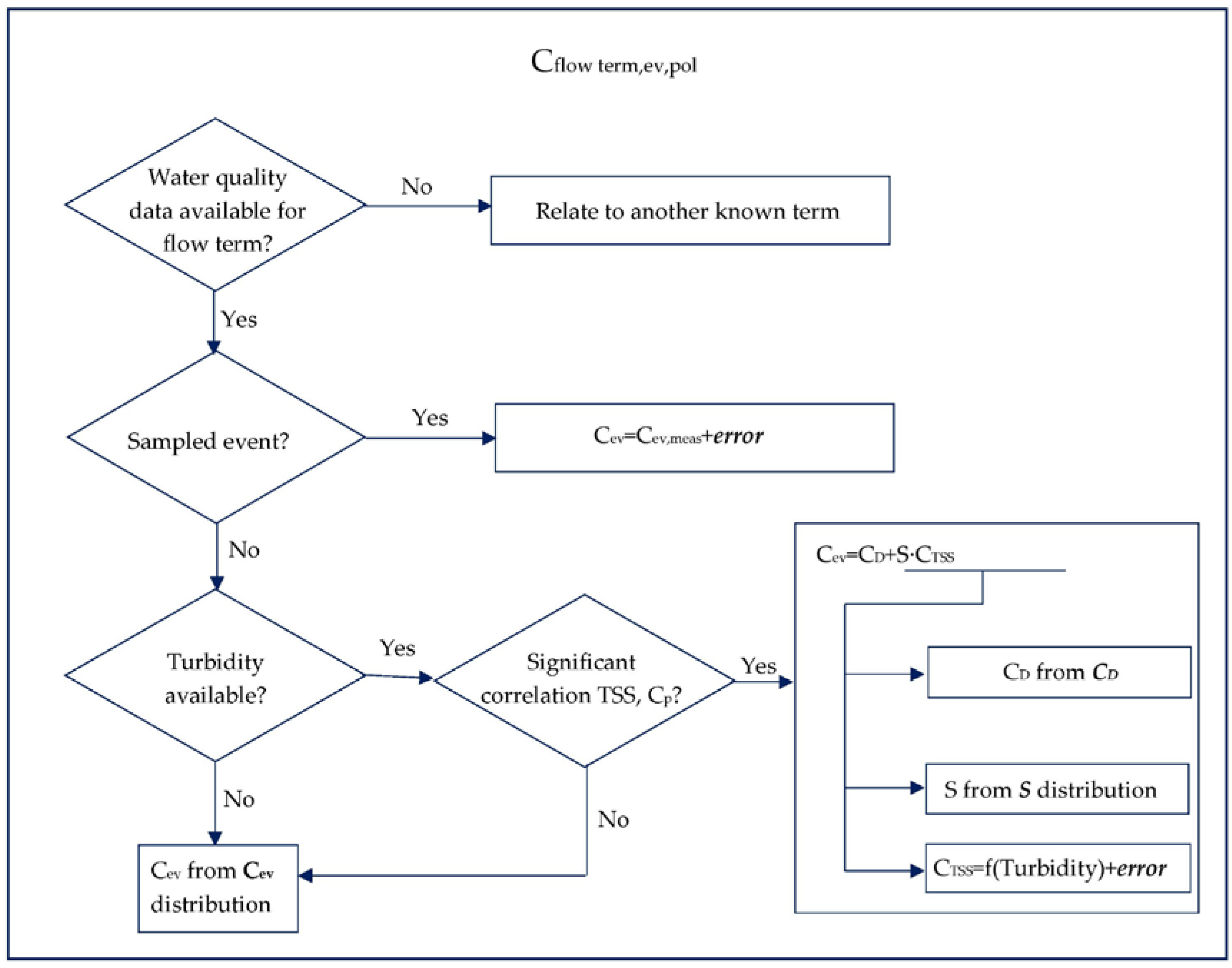
2.2.1. Loads Associated with Water Flows

The overall loads associated with each water flow term ( M i n , R R ,   M o u t , d r a i n and M o u t , o v e r ) were evaluated by summing the loads associated with each rain event (Equation (3)) occurring during the period.
M = e v = 1 n e v V e v C e v
where M is the load over the full period, Vev is the flow volume for a given event, Cev is the event mean concentration for the event and nev is the total number of events during the period.
The generalized methods used for determining the volume and concentration associated with each event for the different flow terms are summarized by Figure 3 and Figure 4 respectively; specific methods used for each flow term are detailed in the sections that follow.

Separation of Rain Events

Events were defined as beginning with the first recorded rainfall at an on-site rain gauge with a resolution of 0.2 mm. A minimal period of 60 min (the average time required for flow to begin in the BFS drain following the beginning of rainfall) was defined as separating two events. The event was considered to be finished when no rainfall was recorded over this hour and the outflow from the BFS drain was equal to at most 0.5% of the recorded volume since the beginning of the event. It was not possible to wait for flow to stop entirely in the BFS drain to define the end of events, as flow continued at low rates for many hours following the end of rainfall. The fraction of 0.5% was chosen, following a sensitivity analysis, as a compromise which attributed most BFS drain flow to events (91%) without creating excessively long events. In order to ensure that the period’s full BFS drain volume was accounted for, the series was multiplied by the inverse of the fraction counted within events (×1.1).

Min,RR 

Comparison of rainfall with RR runoff volumes showed a highly variable runoff coefficient, often exceeding one, indicating that the road surface catchment was not clearly divided and the contributing surface varied between rain events (most likely as a function of rainfall condition). These data were thus judged not to be representative of flows entering the BFS, nor sufficiently reliable to calibrate a model. They were only used to evaluate event mean turbidity concentrations.
Therefore, for each event, the inflow volume (Vin) was evaluated using a simple initial loss reservoir model [25], with a depth SI, that empties by evaporation and generates runoff by overflow. It was applied to the impermeable road surface catchment using on-site rain data and local evapotranspiration measurements from Météo France. As the initial losses could not be calibrated, its depth SI was varied stochastically between 0.4 and 1 mm, values typical of a new road surface such as that in Compans [26,27].
For sampled events, which covered 124 mm of the 610 mm of rainfall in the 13 month period considered, measured total concentrations were applied, varying analytical errors stochastically, assuming normal distributions (Appendix B, Table A1).
According to the non-parametric Spearman correlation test at a 95% confidence level, no correlations were observed between total event mean concentrations of any of the selected pollutants and rain event characteristics (rainfall depth, maximum rainfall intensity, mean rainfall intensity, antecedent dry period). Therefore, concentrations for events outside of these periods were estimated using a stochastic method developed by Hannouche et al. [28], which makes use of continuous turbidity measurements in order to minimize uncertainty associated with the stochastic approach. A linear regression was established between TSS measurements from sampled events and corresponding volume-weighted event mean turbidities calculated from continuous measurements (Appendix C). When valid turbidity measurements were available, a TSS concentration was calculated from the volume-weighted event mean turbidity, including a randomly selected error assuming a normal distribution of residuals from the regression (Table A2). As it is likely that this relationship is no longer linear for very small turbidity values, when turbidity was below the lowest event mean turbidity (50 FNU) measured for sampled events, TSS values were selected in a uniform distribution between zero and 70 mg/L (the corresponding lowest event mean TSS concentration). For pollutants for which particulate concentrations in water are correlated with TSS (P < 0.05 according to the non-parametric Spearman test, a hypothesis which was retained for all pollutants except NP), total concentrations were estimated according to Equation (4). When valid turbidity data was unavailable or when particulate concentrations in water did not correlate with TSS concentrations, Cev was directly sampled from the pollutant’s total concentration distribution.
C e v = C D , e v + S P , e v C T S S , e v
where Cev is the estimated event mean concentration (g/L), CD,ev is a randomly sampled value in the pollutant’s dissolved concentration distribution (g/L), SP,ev is a randomly sampled value in the pollutant’s solid particulate concentration distribution (g/g) and CTSS,ev is the TSS concentration estimated from the turbidity measurement (g/L).
As pollutant concentrations in stormwater tend to follow log-normal distributions [29], experimental measurements of Cev, CD,ev and SP,ev were first tested for log-normality by a Shapiro-Wilk test on log transforms using a limit of P < 0.05. If the hypothesis of log-normality was rejected, the data set was tested for normality. The hypothesis of log-normality was only rejected for dissolved concentrations of OP, for which the hypothesis of normality was not rejected. The distributions employed for each pollutant are described in Appendix B (Table A3).
An additional source of uncertainty related to inlet mass calculation is the representativity of water samples. This uncertainty is associated with both the efficiency of sampling (whether the event mean sample accounts for the full event) and with sampling from a reference catchment rather than sampling the real inlet water. As it is difficult to quantify the effects of this latter uncertainty, which is likely dominant, these sources of uncertainty were not accounted for. As such uncertainties associated with inlet mass calculations may be slightly underestimated.

Mout,drain 

As with RR, concentrations were measured in the BFS drain for some events; in this case, the sampled events represented 145 mm out of the 610 mm of rainfall over the studied period. Again, measured concentrations were used where possible, stochastically accounting for analytical uncertainty. When either the dissolved or particulate concentrations were below the LoQ, the concentration in the given phase was selected in a uniform distribution between 0 and the LoQ and the total concentration was calculated as the sum of total and dissolved concentrations.
At this location, turbidity was not measured continuously as the particulate fraction of pollutants was expected to be less significant, an assumption that was confirmed through the measurement campaigns [23]. Therefore, for most pollutants, outlet concentrations were randomly sampled within the log-normal (P < 0.05) total outlet concentration distributions (Table A4).
A different approach was used for Phen and Pyr, which were frequently found to be below the limit of quantification (LoQ) in the dissolved and/or particulate phases. In this case, particulate concentrations were treated separately from dissolved concentrations. For each event, a choice as to whether a concentration was below the LoQ was made randomly, assuming the probability of a dissolved or particulate concentration being beneath the LoQ to be equal to the proportion of samples with measurements below the LoQ for the parameter. If the parameter was chosen to be below the LoQ for a given event in a given phase, its concentration was selected in a uniform distribution between zero and the LoQ. Otherwise, its concentration in the given phase was selected from the distribution of measurements above the LoQ. A log-normal distribution was used in the particulate phase for both pollutants and for the dissolved phase of Pyr; as Phen was only measured in the dissolved phase in 4 samples, a uniform distribution was used (Table A4). The total concentration is taken to be the sum of the dissolved and particulate phase concentrations.
For most of the period, drain outlet volumes were evaluated using continuous flow measurements; the only source of uncertainty was that associated with this measurement, which was assumed to be normally distributed. However, data was not available between the beginning of operation of the BFS (18 March 2016) and the installation of the flow meter (6 April 2016). Outflow volumes for this period were reconstructed by multiplying the event input volume by a randomly selected value from the log-normal (Shapiro-Wilk P < 0.05) distribution of the ratio of drained volume to input volume (runoff and direct rainfall) from the period with available measurements before the installation of the check dams.

Mout,over 

Concentrations in the system overflow were not measured experimentally. It was therefore assumed that overflow concentrations for each event were related to the corresponding inflow concentrations according to the Equation (5), which assumes that the BFS acts as a well-mixed reservoir over the event duration, that the rainfall itself is not a source of pollutant mass and that no sedimentation or erosion occurs. Both because sedimentation may occur in a system of this type and because most overflow will occur later in rain events after the first flush of pollutants [30], this hypothesis likely leads to an overestimation of overflow mass, the effects of which will be discussed later.
C o v e r , e v = C i n , R R , e v   V R R , e v V R R , e v + h r a i n , e v A B F S
where Cover,ev is the total pollutant concentration for a given event (g/L) and Cin,RR,ev, VRR,ev and hrain,ev are the total concentration in road runoff (g/L), the volume of road runoff (L) and the rainfall depth associated with the same event (mm), respectively and ABFS is the biofiltration swale surface area (m2).
Experimental measurements of overflow were available from November 2016–April 2017. For this period, uncertainty in the overflow volume was considered to be due to the uncertainty in the measurement of water depth at the V-notch weir. An error in this depth was selected randomly assuming its relative error to be normally distributed and then used to calculate a volume error (Table A2).
Overflow for the period from March–November 2016 had to be estimated. To do so, the event inflow volume ( V R R , e v + h r a i n , e v A B F S ) was compared to the storage volume available at the surface of the BFS. When the event volume was smaller than the storage volume, Vover was assumed to be null. When this was not the case, Vover was calculated according to Equation (6). This model was validated for the period during which overflow data was available; measured overflow volumes were within the predicted range for 134 of the 139 events for which data was available.
V o v e r , e v = V R R , e v + h r a i n , e v A B F S V d r a i n , e v Δ V m e d i a , e v
where Vover,ev is the volume of overflow (L), VRR,ev is the volume of RR (L), hrain,ev is the total rainfall depth (mm), ABFS is the biofiltration swale surface area (m²), Vdrain,ev is the drain outflow volume (L) and ΔVmedia,ev is the evolution in the water stored in the filter media (L). For each event, ΔVmedia,ev was randomly selected in a uniform distribution between 0 and field capacity of the full BFS.

2.2.2. Mass Stored in Soil

The variation over the 13 month period of the mass of each pollutant pol stored in soil was calculated according to Equation (7).
M s o i l , f i n a l M s o i l , i n i t i a l = i = 1 8 j = 1 3 ( S s o i l , i , j S s o i l , i n i t , i , j ) × V s o i l , i , j × ρ s o i l , i , j × f s o i l , < 2 m m , i , j
where Msoil,final and Msoil,initial are the masses of the pollutant stored in the soil at the end and at the beginning of the study, respectively (g), the volume of the soil is divided into 24 different sub-volumes corresponding to i = 8 zones (2 to 3 zones in each of the 3 BFS sections) and j = 3 depth layers (0–5 cm, 5–15 cm, 15–50 cm), Ssoil,i,j is the final concentration of the pollutant pol in the <2 mm fraction attributed to zone i and depth j (g/g), Ssoil,init,i,j is the initial concentration of the pollutant pol in the <2 mm fraction attributed to zone i and depth j (g/g), Vsoil,i,j is the volume of soil in the sub-volume i,j of the BFS (L), ρsoil,i,j is the bulk density of the filter media (g/L) and fsoil,<2mm,i,j is the mass fraction of the soil with particles less than 2 mm.

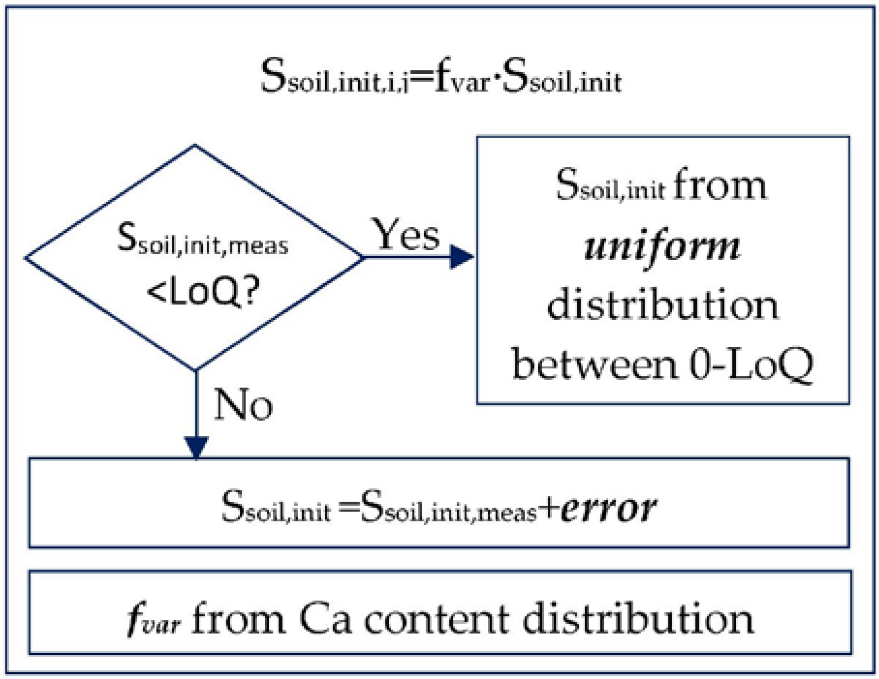
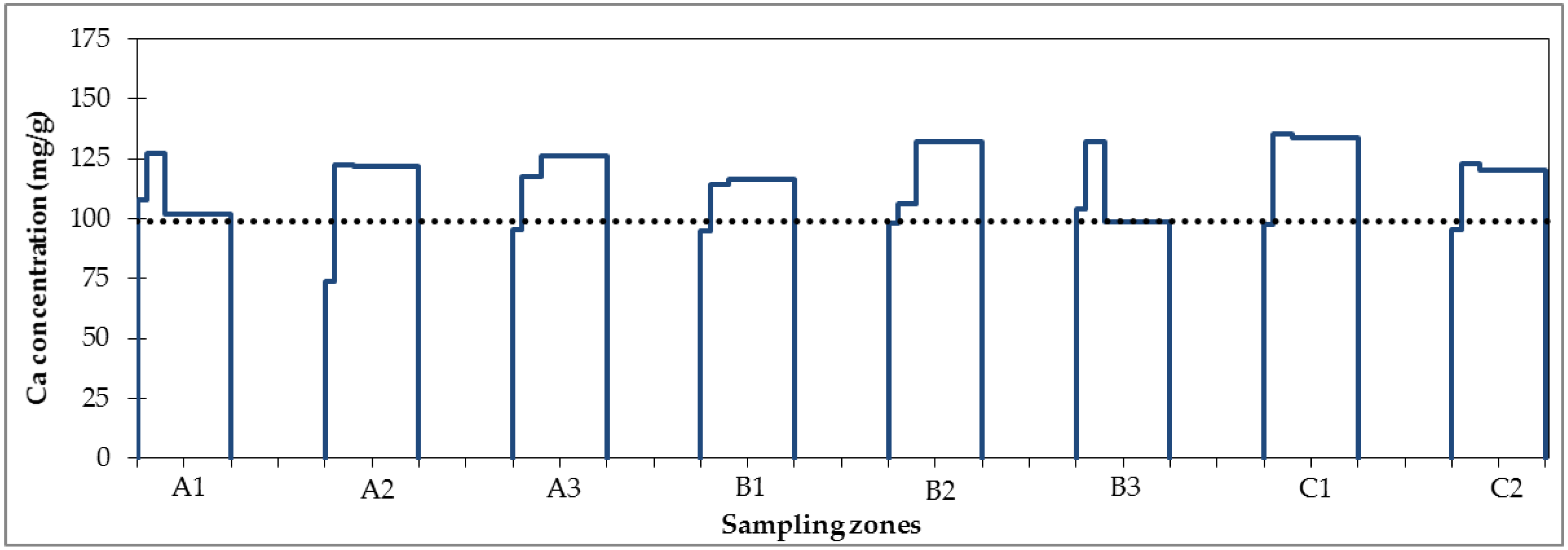
Definition of Soil Properties

The BFS sub-volumes i,j were defined according to the soil sampling strategy applied in April 2017.
As previously mentioned, at the end of the study, the filter media was sampled by first characterizing surface contamination and defining 2–3 zones of similar surface contamination (from a most contaminated to a least contaminated zone) in each of the three BFS sections separated by check dams (Figure 2). A composite core was than sampled for each zone i and separated in 3 depth layers j.
An analytical error in the final concentration of each pollutant (Ssoil,pol,i,j) was randomly selected for each iteration. The resulting concentration was then attributed to the soil mass associated with a corresponding sub-volume of soil (Vsoil,i,j, Equation (8)).
V s o i l , i , j = f i V s e c t i o n h j h c o r e
where Vsoil,i,j is the sub-volume assigned to sample i,j in the soil pollutant mass calculation (L), Vsection is the volume of soil in the section (L), fi is the fraction of the surface area of the section applied to zone i, hj is the soil depth of the layer j of the core (cm) and hcore is the soil depth of the core [cm], equal to the depth of the biofilter’s filter media.
This sampling strategy relies on the hypothesis that surface contamination from metals is correlated with contamination from each pollutant at greater depths. For each section, pollutant and depth, this hypothesis was evaluated by comparing the ranks of surface concentrations with the ranks of composite core concentrations for the same zone. Figure 5 demonstrates the distribution of a pollutant for which the zones were often representative (Cu) and a pollutant for which the zones were not representative (BPA).
The method for assigning a mass of soil to each sample is described in Figure 6. When ranks between surface contamination and composite core contamination were identical, fj was assumed to be equal to the proportion of the section surface area covered by the zone. In this case, uncertainty due to the subjectivity of identifying the boundaries of each zone was accounted for by randomly selecting an error for each zone’s surface area in a uniform distribution between ±10% of the total section surface area, such that the sum of zone areas in each section remained constant (Table A5).
When the ranks of concentrations at a given depth were different from those at the surface, the zones were assumed not to be representative of the distribution of contamination. Therefore, the composite cores were treated as random samples, each equally representative of the entire surface in the section. In this case, fi was selected in a uniform distribution between 0 and 1, such that the sum of fractions for each zone were equal to 1.
For each V s o i l , i , j thus defined, a density was selected using mean densities for each depth, choosing an error within a uniform distribution of ±20%, as the hypothesis of a normal or log-normal density distribution was rejected.
Because pollutant analyses were carried out on the fraction <2 mm and the filter media contained a non-negligible fraction of >2 mm particles, which were included in bulk density measurements but unlikely to contain as many pollutants as smaller particles due to their mineral character and low surface area. The mass of soil was therefore corrected by this factor. As the hypothesis of normality was not rejected for this fraction, its value was selected from a normal distribution for each sample (Table A5).

Definition of Ssoil,init,i,j

The initial concentration of each pollutant in the soil was estimated by analysing all pollutants in a sample of filter media taken before its installation in the BFS. In the mass balance calculation, an analytical error in the initial concentration of each pollutant was randomly selected for each iteration. When initial concentrations were below the LoQ, initial concentrations were randomly selected in a uniform distribution between 0 and the LoQ.
An additional source of uncertainty is the representativeness of the initial filter media sample for each portion of the BFS due to imperfect mixing of topsoil and sand to produce the initial filter media at the time of construction. As the filter media in this system is composed of topsoil with low calcium content (0.3%) and lime sand containing 38% calcium, calcium may be considered to be a tracer of the sand, which can be used to evaluate the heterogeneity of mixing of the filter media. Calcium content varied by a relative standard deviation of 13.8%, indicating an imperfect homogenization of the two materials during media fabrication (see Appendix D for the calcium distribution). Therefore, a factor of variability fvar, equal to the variability of calcium in the media cores sampled in the BFS, was applied to the initial concentration of each pollutant in order to estimate the uncertainty in the initial pollutant mass due to the variability in the filter media’s composition. As the hypothesis of the normality of the calcium content distribution was not rejected (Shapiro-Wilk P < 0.05), this factor was randomly selected in a normal distribution with the relative standard deviation of calcium measured in all soil samples.
A different factor of variability was applied to each sub-volume i,j of the BFS (Figure 7).

3. Results and Discussion

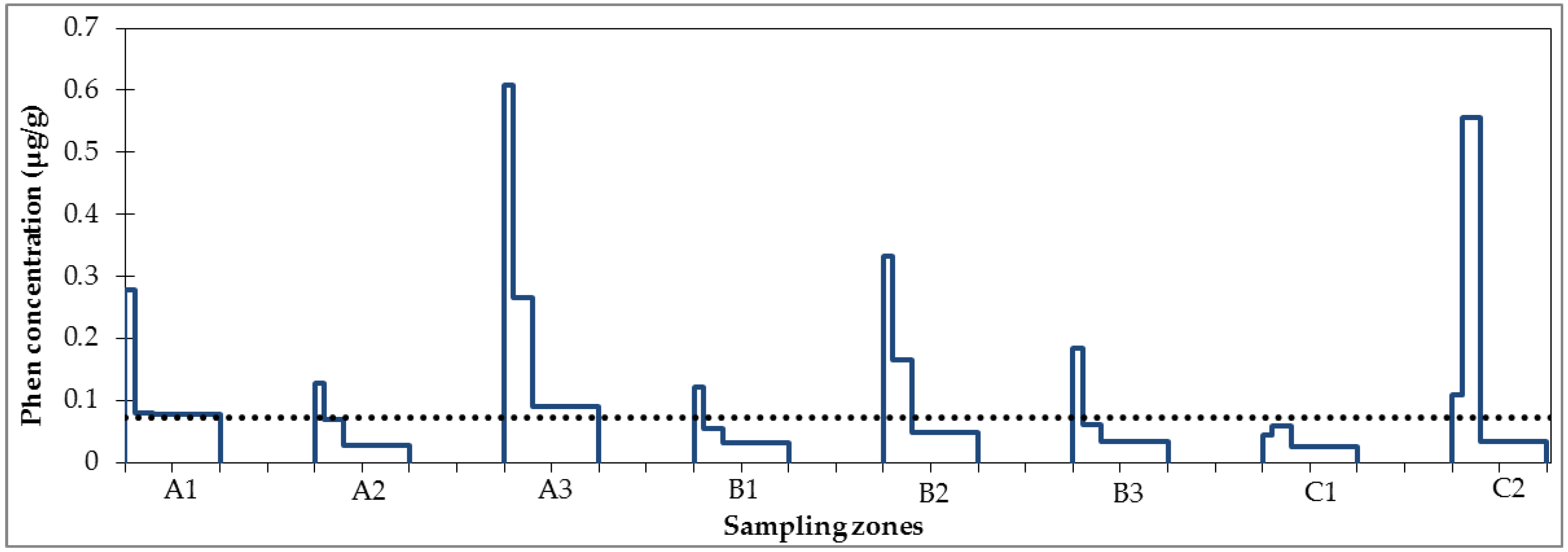
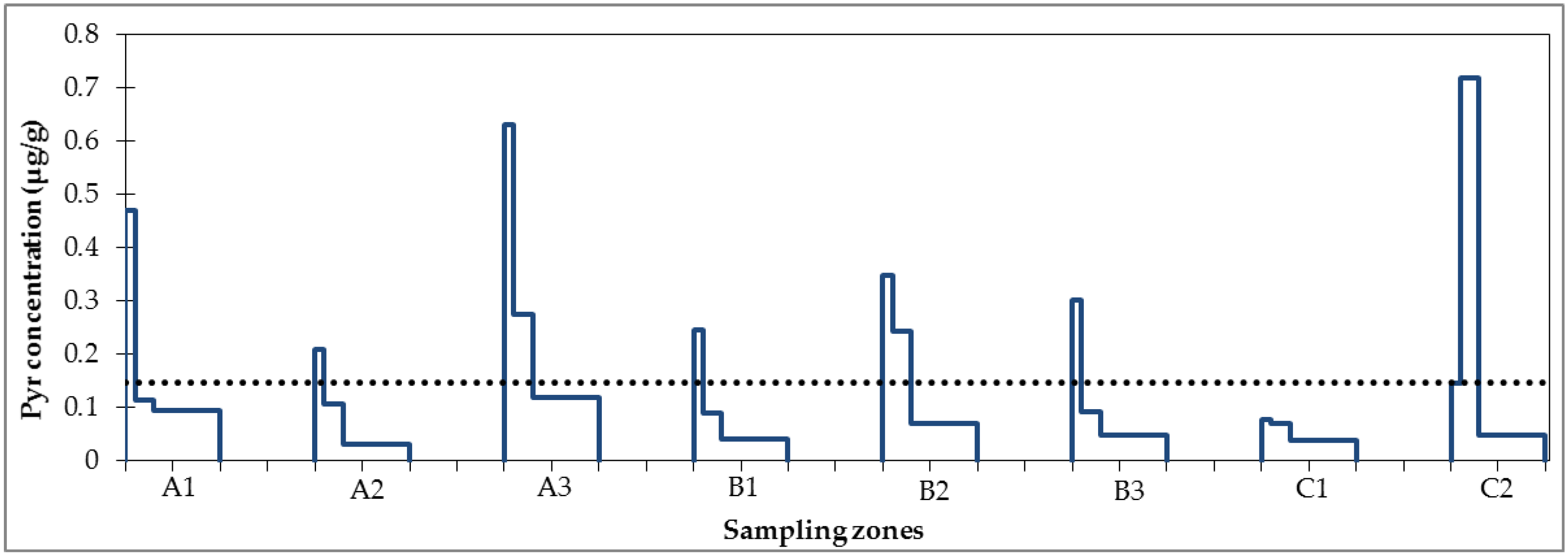
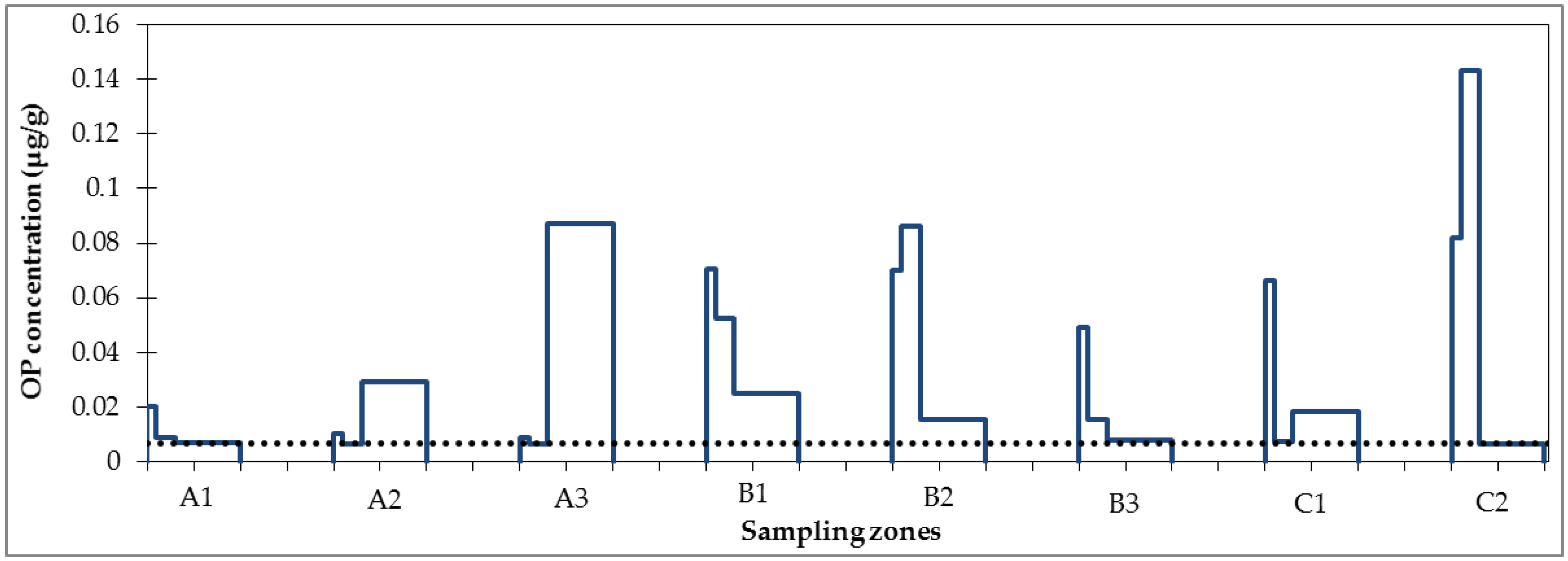
3.1. Micropollutant Load in Road Runoff

The calculated micropollutant loads in untreated road runoff are summarized in Table 3. The median annual Cu load per road surface area (851 g/ha/year) is high compared to most values issued from a review of annual traffic area runoff loads (median 355, with values ranging from 34–3780 g/ha/year), while that of Zn (2360 g/ha/year) is slightly below the median (2600 g/ha/year) issued from the same data set [31].
Annual NP and DEHP loads (7.87 and 77.3 g/ha/year, respectively) are lower than those of 22 and 350 g/ha/year, respectively, calculated for a highway with much higher daily traffic by Björklund et al. [32]. This may be due to traffic differences as well as to a decrease in the use of these compounds following their identification as priority pollutants by the European Union [2]. Both NP and OP (2.15 g/ha/year) annual loads exceed those evaluated for runoff from a residential urban catchment (1.9 and 0.12 g/ha/year, respectively) [33].
The BPA load evaluated per active surface and mm of rainfall (4.92 mg/act.ha/mm) is similar to values calculated by Hannouche et al. [28] for runoff from three different urban catchments in separate storm sewers (4.2–5.9 mg/act.ha/mm), while those of NP and especially OP (18.6 and 5.06 mg/act.ha/mm, respectively) exceed corresponding loads from the same study (12–13 and 0.87–1.0 mg/act.ha/mm). These results are coherent with previous research which has shown tires to be a major source of OP and several automobile components to be sources of NP [34].
Distributions of calculated loads are slightly skewed to the right, with confidence intervals reaching between 13–22% in the negative direction and to 17–41% in the positive direction. Uncertainties in water volume calculations account for about 4% in the negative direction and 6% in the positive direction, indicating that pollutant concentration estimations are the main source of uncertainty. The DEHP load has the highest relative uncertainty, followed by Phen, Pyr, Zn, NP, OP, Cu and BPA.

3.2. Micropollutant Load Reduction

Median estimations of the integrated pollutant load reduction by the BFS system over the mass balance period vary between 27–72% depending on the pollutant (Table 4). Load reductions in biofiltration systems are typically higher than concentration reductions due to water volume reduction [6]. In this case, however, load reductions of the full system tend to be lower than median concentration reductions of drained water, which are summarized in Table 4 and have been reported in detail elsewhere [23].
The main reason for this is that even though about 21% (15–24%, 95% confidence interval) of runoff volume is dissipated by the system (likely due to evaporation/evapotranspiration), around 35% of this volume (31–37%) overflows. This high proportion of overflow volume indicates that water quality performance could be improved by increasing the system’s water treatment capacity, either by increasing its surface storage volume or by increasing the rate of treatment by increasing its surface area or using a filter media with a higher hydraulic conductivity. Indeed, the hydraulic conductivity of the present system (21 mm/h) is relatively low compared values typically recommended in biofiltration design guidelines (for example, 100–300 mm/h in Australian guidelines [35]).
We also note that much of the overflow occurred during the first three months of operation, when the check dams were not yet installed and exceptional rainfall occurred. Indeed, 253 mm of the 610 mm of rainfall in the full period occurred during these three months (see Figure A1, Appendix A). Rainfall during the first period included two events with 2-year return periods, while no events outside of the initial period exceeded a return period of six months. Measurements made after check dam installation show a lower proportion of overflow, due both to the absence of particularly intense events and to the increased surface storage volume.
As the calculation assumes that the only improvement to overflowed water quality is due to its dilution by rain falling directly on the BFS, the overflow mass accounts for between 20–29% of input mass. As some sedimentation is likely to occur in the BFS before overflow, this term may be overestimated, leading to an underestimation of load efficiency and intercepted mass.
The lowest overflow proportions are observed for TSS; this is likely due to the fact that RR turbidity and therefore calculated TSS, tended to be lower for the high-volume events generating overflow, particularly during May 2016 (before check dam installation, see Figure A1 in Appendix A) when the stock of mobilizable particles on the road surface seems to have been depleted. The highest overflow proportions are observed for pollutants that were less strongly associated with the particulate phase (BPA and OP) and for NP, for which turbidity was not used to estimate unmeasured concentrations as its particulate concentrations were not found to be correlated with TSS. This may be indicative of a bias in these calculations. Indeed, for sampled events during this period, dissolved pollutants were also observed at low concentrations; however, without a relationship to a continuous water quality measurement, concentrations of unsampled events were selected randomly from the total concentration distribution.
Outlet loads from the drain account for between 7 and 51% of inlet loads to the BFS, depending on pollutants. For example, drained TSS accounts for 13% (9–16%, 95% confidence interval) of inlet TSS. At first glance, this value appears high, given that only 45% (41–52%) of runoff was drained from the BFS and the median TSS concentration reduction was found to be 92%. Indeed, event pollutant load reductions would be higher for events with high concentration reductions; however, higher outlet TSS concentrations, corresponding to lower concentration reductions, were observed for some events during a winter period [23]. This inter-event variability in outlet water quality is responsible for the lower load reduction over the full period than those that may be observed for most events. Poor performance was observed for all pollutants during some events in the winter period and/or during the beginning of operation (see Ec values in Table 4). As these values are accounted for in the outlet pollutant concentration distributions used to estimate loads, the over or underrepresentation of events with poor performance in the sampled events could be a source of bias in pollutant load calculations. Continuous monitoring of drained water turbidity would be one method for reducing this potential bias, at least for pollutants found to be mainly present in the particulate phase.

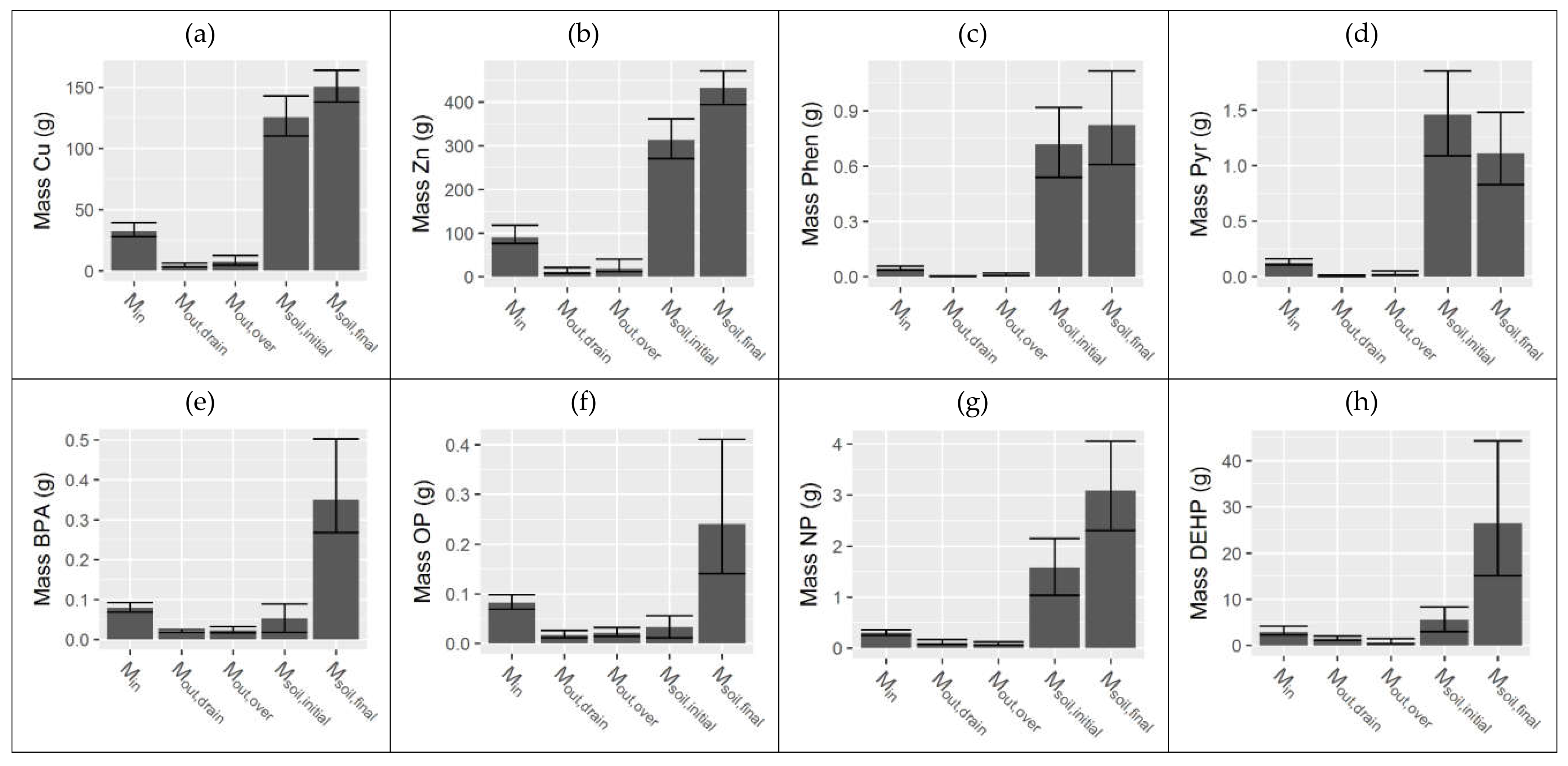
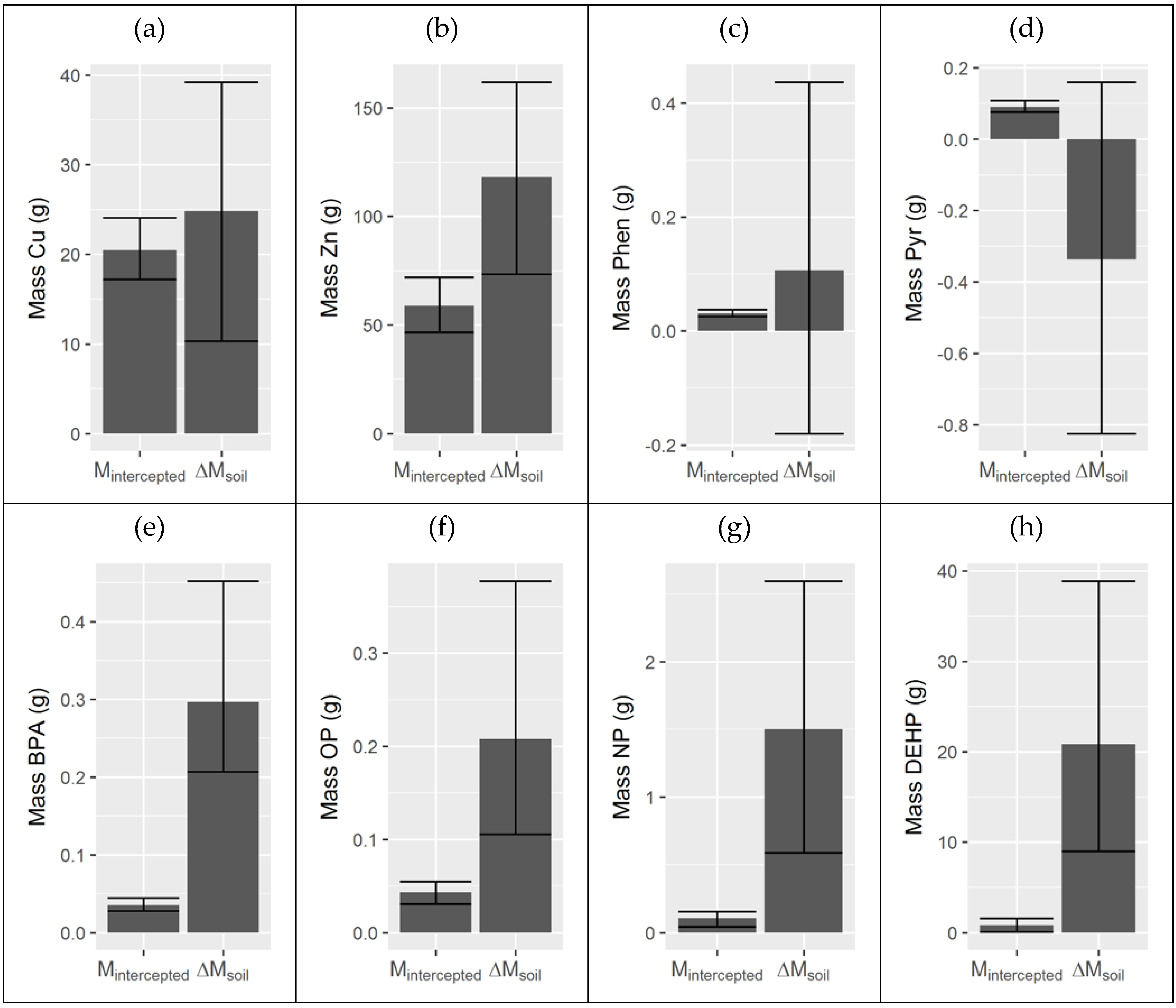
3.3. Integrated Water and Filter Media Mass Balance

All mass terms associated with water fluxes (Min, Mout,drain and Mout,over) and soil (Msoil,initial and Msoil,final) are presented in Figure 8. They are also provided numerically in Appendix E. A first observation may be that the soil mass terms, even at the beginning of the study, are much greater than the load terms for Cu, Zn, Phen, Pyr and NP. An important implication of this fact is that the absolute uncertainties in calculated soil masses are large compared to the load terms, sometimes even exceeding the loads entering the system. This may limit the possible interpretations of the mass balance and will be discussed in detail later.
It can also be observed that relative uncertainties in the soil mass balance terms are highly variable between different pollutants. The highest relative uncertainties are observed for pollutants with concentrations in the initial filter media below the LoQ (BPA, OP and DEHP), for which the 95% confidence interval extended (−66, 70%), (−65, 69%) and (−46, 50%) from the medians, respectively. However, as the initial masses of these pollutants were low, associated absolute uncertainties are small compared to other pollutants. Beyond this, relative initial mass uncertainties increased with increasing analytical uncertainties from as little as (−12, 14%) for copper to (−34, 37%) for NP.
Relative uncertainties in the final soil mass vary between pollutants due not only to analytical uncertainty but also to the distribution of each pollutant throughout the filter media (see Figure 5 and Appendix D) compared to that of trace metals at the surface, which determined the algorithm used for evaluating Msoil,final. As the distribution of all organic micropollutants often differed from that of trace metals at the surface, the second method, which involves more uncertainty, was frequently employed. Cu and Zn have the lowest relative uncertainties in final mass (−8, 9%) and (−9, 9%), respectively, while the highest are observed for OP and DEHP (−41, 71%) and (−43, 68%).
As previously discussed, Min exceeds the sum of Mout,drain and Mout,over for all pollutants, indicating that a certain mass has been intercepted by the filter media. At the same time, the mass stored in the soil increased for most pollutants over the study period. The intercepted mass of each pollutant (Mintercepted) is compared to the evolution in the mass of pollutant in the soil (ΔMsoil) in Figure 9. In a perfectly conservative mass balance, in which all important sources and sinks are correctly represented, these two terms are expected to be equivalent. ΔMsoil < Mintercepted would correspond to an unrepresented sink for pollutant mass (dissipation), whereas ΔMsoil > Mintercepted indicates that there is a source of the pollutant that was not accounted for in the mass balance. Results in this comparison vary greatly between pollutants.
While the median value of Mintercepted is lower than that of ΔMsoil for Cu, the confidence interval of Mintercepted is completely contained within that of ΔMsoil, which is notably larger. These results are thus compatible with the hypothesis that the important terms in the Cu mass balance are accurately represented.
The confidence interval of ΔMsoil for Phen and Pyr also encompasses that of Mintercepted. However, in this case, ΔMsoil is not significantly different from zero, with confidence intervals for both pollutants spanning from negative to positive values. As such, given the level of uncertainty in ΔMsoil, it is impossible to draw any meaningful conclusions as to the fate of these pollutants in the soil from the mass balance.
ΔMsoil is higher than Mintercepted for Zn, DEHP, BPA, OP and NP with no overlap of confidence intervals. In this case, although the ΔMsoil interval is wider than that of Mintercepted, the differences between the masses are so large that they are significantly different. Possible explanations for these observations will be explored in the following section.

3.4. Limitations of the Proposed Mass Balance Approach

When ΔMsoil significantly exceeds Mintercepted, at least one of the following must be true: (a) Msoil,initial and/or Min has been underestimated, (b) Msoil,final, Mout,drain and/or Mout,over has been overestimated and/or (c) important source terms have been ignored. The purpose of this section is to evaluate possible explanations for the ΔMsoil > Mintercepted observations for Zn, BPA, OP, NP and DEHP.

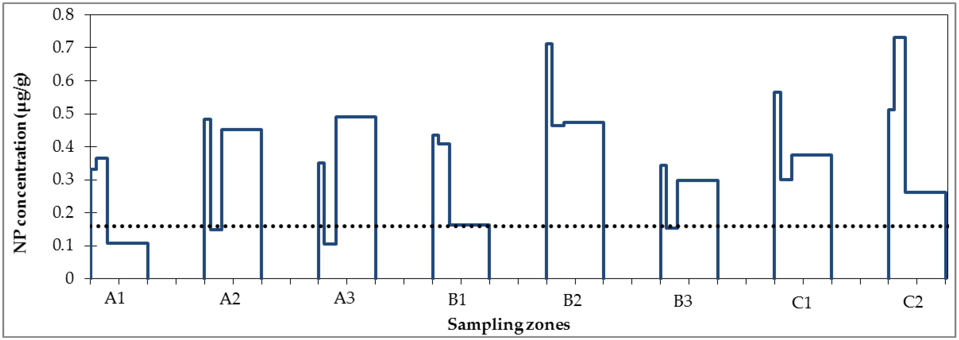
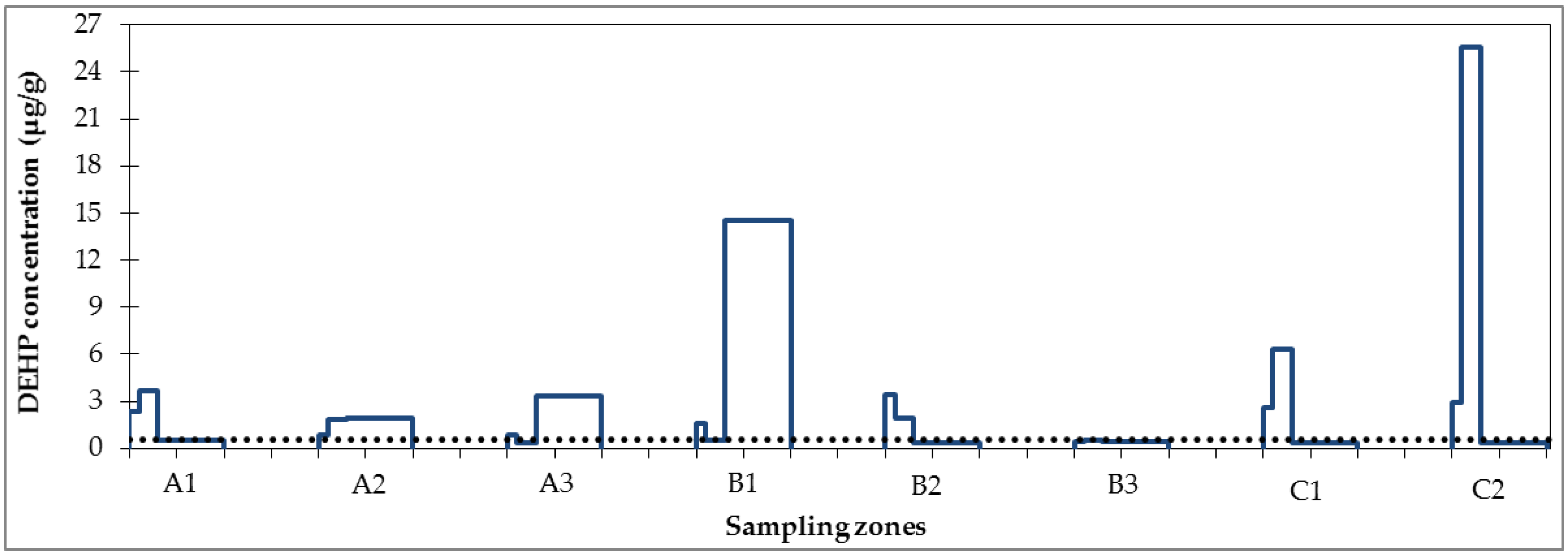
3.4.1. Questionable Representativity of the Initial Soil Sample

For all pollutants, possible errors in soil mass calculations (including analytical uncertainties but also variability in the soil properties throughout the system and the representativity of each sample) have been accounted for in the calculation.
The representativity of the initial soil sample, which was collected in the pile of prepared filter media during construction, might be questionable due to construction methods leading to variations in the filter media composition throughout the BFS. Imperfect topsoil and sand mixing were taken into account by varying initial concentrations throughout the filter according to the relative variability of Ca, a tracer of the lime sand. Another source of uncertainty is the quality of the initial topsoil itself, which may vary within or between truckloads. While it appears unlikely that Msoil,initial is biased to such an extent that it exceeds the already large variability allowed for in the mass balance calculation, it is highly recommended that future studies account for the fact that filter media is likely to be heterogeneous. Initial samples should be taken at various locations in the filter media immediately after construction or taken at different moments during filling. Samples could either be analysed separately, which would allow for a characterization of spatial variability or used to form a composite sample.

3.4.2. Overestimation of Outlet Pollutant Loads

One potential bias in the load calculation comes from the estimation of the concentrations in the overflow. As this concentration was not measured directly, it was assumed to be equal to the inlet concentration, accounting for a dilution by direct rainfall. As previously mentioned, the assumptions that no sedimentation occurred at the surface of the biofilter and that water quality was constant throughout the rain event, both used in this estimation, likely lead to an overestimation of Mout,drain.
Another source of bias is the representativity of sampled rain events for the full period. While sampled rain events covered various seasons and hydrologic conditions, they also tended to correspond to rather large events. The use of a continuous turbidity measurement in calculating inlet pollutant loads not only decreases uncertainty but also allows the adjustment of inlet concentrations to real observations for each event, minimizing this bias. Indeed, the median inlet masses calculated using the turbidity measurement are slightly lower than those calculated using random sampling from the total concentration distribution (Appendix F). This indicates that the distribution of inlet concentrations for sampled events tends to be higher than that of all events in the period. While this was corrected for inlet loads, a similar continuous measurement was unavailable for outlet concentrations from the drain, which may be a potential source of bias. Although this bias could lead to either an overestimation or an underestimation of pollutant load, in the present case, an overestimation is suspected.
In order to test whether an overestimation of Mout,over and/or Mout,drain might explain the significant differences between Mintercepted and ΔMsoil for Zn, BPA, OP, NP and DEHP, we consider the limiting hypothesis that both outlet terms are equal to zero by comparing ΔMsoil with Min in Appendix G.
It can be seen that ΔMsoil is significantly larger than Min for BPA, OP, NP and DEHP. Therefore, an overestimation of outlet terms cannot explain the fact that ΔMsoil > Mintercepted for these pollutants; there must be a source of these pollutants which was not accounted for in the mass balance. In the case of Zn, the Min confidence interval intercepts that of ΔMsoil, albeit at the lower end, meaning that an extreme overestimation in the outlet terms could explain the difference between Mintercepted and ΔMsoil. However, as neither Mout,over nor Mout,drain is likely to be null, it remains probable that another source of Zn is present.

3.4.3. Atmospheric Deposition

Direct atmospheric deposition on the BFS surface was not accounted for in the mass balance calculations and is another possible source of pollutants in the soil. However, as the surface of the BFS is only 4.5% that of the surface which it drains, the mass associated with direct atmospheric deposition would be much smaller than those associated with runoff even if atmospheric deposition was the main source of pollution in runoff. In addition, a parallel study of the same site which characterized the contamination of atmospheric deposition for Cu, Zn, Phen and Pyr showed it to have concentrations an order of magnitude below those found in road runoff (see Appendix H for more details) [36]. Therefore, accounting for atmospheric deposition would not significantly modify the results of the mass balance in the present case.

3.4.4. Galvanized Steel Barrier

A potential source of Zn, which was not accounted for in the mass balance, is a galvanized steel safety barrier that separates the BFS from the road (see Appendix I for a photograph of the barrier). As rain falls on this barrier, it is likely to emit zinc; in addition, a portion of the runoff from the road is in contact with its posts as it enters the BFS. Although a similar barrier is also in place along the roadside where untreated runoff is collected, it is located on the opposite side of the curb and does not have the same amount of contact with runoff. Therefore, inlet loads based on data from the reference catchment do not account for this source, which probably explains at least part of the excess zinc found in the soil.

3.4.5. Degradation of Ethoxylated Alkylphenols

One potential source of alkylphenols (OP and NP) in the BFS is the degradation of alkylphenol ethoxylates (APEO). Indeed, alkylphenols and short-chained APEO (OP1EO, OP2EO, NP1EO and NP2EO) are the stable by-products of the degradation of industrially-produced, longer-chained APEO [37], for which tires, plastic vehicle components, paints, lubricant oils and asphalt are all potential sources in road runoff [38]. Therefore, if these longer-chained APEO, which were not analysed in the present study, are present in runoff, their degradation after retention by the BFS is likely to produce NP and OP in the BFS, which may at least partially explain the excess of these contaminants found in the soil.

3.4.6. Biofiltration Swale Construction Materials

The significant excesses of BPA, NP, OP and DEHP found in the BFS soil may also be the result of emissions from various materials used to construct the BFS, including a geomembrane liner, a drain, a fabric surrounding the drain and asphalt. Emissions tests of these materials were conducted in batch experiments and have been detailed elsewhere; the tests showed that all four of these pollutants could be emitted one or more of these materials [12]. Because the geomembrane, drain fabric and drain were located below or surrounding the filter media, these sources may also explain the high concentrations observed in the lower portions of the filter for these pollutants (Figure 5 and Appendix D).
Insofar as additional pollutant sources come from materials used in the device itself, the high ΔMsoil compared to Mintercepted indicates that the removal of these pollutants from runoff comes at a high environmental cost in terms of soil pollution. For example, the BFS retains 39% of incoming loads of BPA at the cost of emitting nearly 9 times this amount into the soil. If biofiltration devices are to be part of an integrated strategy for limiting pollution, it is important to limit the use of materials likely to emit the very pollutants being treated. As many organic micropollutants are ubiquitous in industrially-produced, synthetic materials, it is likely to be difficult to find drainage or impermeabilization materials that do not include them.

3.5. Necessary Conditions for a Mass Balance Significantly Demonstrating Dissipation

The previous discussion highlights many of the methodological difficulties associated with establishing an in situ mass balance, including high uncertainties, potential biases and uncharacterized sources. The purpose of the current section is to establish a list of necessary conditions for establishing a mass balance capable of demonstrating dissipation with certainty. For the purposes of this discussion, we define an indicator of the proportion of intercepted pollutant mass dissipated in the system, Esoil (Equation (9)).
E s o i l = 1 Δ M s o i l M i n t e r c e p t e d
where Esoil is the percent difference between the mass of pollutant recovered in the system at the end of the period compared to the mass of pollutant intercepted, Δ M s o i l is the change in soil mass over the study period and M i n t e r c e p t e d is the mass of pollutant intercepted by the biofilter over the study period.
A significant dissipation may be observed when Esoil is significantly greater than zero. This is not the case for any of the organic micropollutants considered in the present study (see Appendix J), despite the fact that many of the studied species are expected to be degraded in soil environments. Indeed, for all pollutants, Esoil is either negative or the uncertainties so large that it is not significant. The necessary conditions for demonstrating a significant dissipation are listed and discussed below, given the lessons from the current study.

3.5.1. Pollutant Loads in and out of the System Have Been Evaluated, Accounting for Uncertainties, for all Important Pollutant Flux Terms

The evaluation of pollutant loads associated with flows in and out of a stormwater biofilter generally requires characterization of both pollutant concentrations and water flows. When not all events in the study period are sampled, pollutant concentrations for unsampled events can be evaluated stochastically. Continuous measurements of turbidity can improve load estimates by correcting for biases in sampled events, at least for particulate pollutants. It is to be noted that continuous measurements require substantial effort for equipment maintenance and data validation.

3.5.2. Both Initial and Final Concentrations in Soil Have Been Evaluated in a Representative Fashion; Soil Properties and Their Variability Have Been Characterized

Obtaining representative soil samples at the beginning and the end of a study presents several challenges. In the initial phase, it should not be assumed that a filter media is perfectly homogenous as it may vary in composition due to imperfect mixing of initial materials (such as topsoil and sand). Soil properties, such as density, may also vary spatially and over time; it is recommended that several measurements be taken at the beginning and at the end of the study period in order to account for potential variability.

3.5.3. No Pollutant Sources are Present within the System or the Dissipation of a Given Pollutant Exceeds Its Production/Emission (in the Second Case, Dissipation Will Be Underestimated but May Still Be Identified)

A major result of the present study is that emissions by synthetic materials within or around a biofiltration device (such as asphalt, drains, drain fabric or geomembranes) may exceed loads associated with runoff. Therefore, ideally, no such materials should be used in systems treating organic micropollutants, especially where a mass balance of organic micropollutants is to be carried out. However, in order to evaluate outlet concentrations, it is necessary to drain water from the filter and in order to measure the full outlet loads from a system, it must be lined to prevent exfiltration. It is therefore advisable to test various materials in order to choose the least polluting one. A longer study duration may also minimize the significance of these emissions in the mass balance, both because emissions are likely to be highest from new materials and because emitted pollutants may degrade over time.
In addition, some pollutants may be the products of the degradation of others. When this is the case, as for alkylphenols, it is unlikely that dissipation can be demonstrated unless the mass balance is expanded to include possible parent compounds, of which there may be many.

3.5.4. Intercepted Pollutant Masses Are Significant Compared to Initial Soil Pollutant Mass

In order for Esoil to be significantly greater than zero (indicating dissipation), its relative uncertainty must be less than 100%, which was rarely the case in the present study (see Appendix J for all relative uncertainties). A better comprehension of the propagation of uncertainties between terms is therefore important for understanding how this may be achieved.
Assuming the errors in load calculations to be independent from those in the soil calculations, the Equation (10), which relates relative errors in Esoil to those in ΔMsoil and Mintercepted, can be derived from the rules of uncertainty propagation [39].
δ r e l , E s o i l = Δ M s o i l M i n t e r c e p t e d δ r e l , Δ M s o i l 2 + δ r e l , M i n t e r c e p t e d 2 E s o i l
when Esoil is positive (as is the case if dissipation occurs), the condition δ r e l , E s o i l < 1 may be applied to this equation to find the necessary conditions for demonstrating Esoil to be significantly greater than zero. Substituting the definition of Esoil, in terms of ΔMsoil and Mintercepted, which are also assumed to be positive, Equation (11) may be obtained. This inequality demonstrates that the larger the relative uncertainties in ΔMsoil and Mintercepted, the larger the difference between Mintercepted and ΔMsoil must be to be significant. Therefore, dissipation will be more difficult to prove when these uncertainties are large.
M i n t e r c e p t e d > ( 1 + δ r e l , Δ M s o i l 2 + δ r e l , M i n t e r c e p t e d 2 ) Δ M s o i l
Because Mintercepted and ΔMsoil are both differences between other mass balance terms, their absolute uncertainties are related to those of the terms used to calculate them. Their relative uncertainties become large when they are small compared the terms used to calculate them (when there is a small difference between two large terms). Therefore, relative uncertainty in ΔMsoil will become large when Msoil,initial is much larger than ΔMsoil. As by definition ΔMsoil must be smaller than Mintercepted for dissipation to occur, we note that the condition in Equation (11) is unlikely to be fulfilled when Mintercepted is much smaller than Msoil,initial due to divergence in ΔMsoil’s relative uncertainty. Uncertainties in Mintercepted itself will also become large if it is small compared to Min due to poor retention, making Equation (11) even harder to fulfil. Besides the efficiency of retention, the magnitude of Mintercepted compared to Msoil,initial also depends on the level of contamination initially in the filter medium, the annual loads of pollutants arriving in the system and the duration of the study.
In the present study, it would have taken 2 years for Mintercepted to approach Msoil,initial for BPA and OP, 6 to 10 years for Cu, Zn and DEHP and at least 19 years for Pyr, Phen and NP. The long duration required for the latter molecules indicates that the soil was initially quite contaminated. Indeed, the initial concentration of NP (0.159 µg/g) was higher than most measurements from a study of 32 soil samples from Ile-de-France, while those of Pyr and Phen (0.146 and 0.072 µg/g, respectively) were in the typical range for the region [40].
The divergence of relative uncertainties is best illustrated by Pyr and Phen (Appendix K), pollutants for which high concentrations were observed in the initial soil sample and for which no sources besides runoff were apparent. In this case, although initial and final soil mass uncertainties were at most ±35%, uncertainties in ΔMsoil reached (−145, 147%) for Pyr and (−269, 310%) for Phen, leading to uncertainties in Esoil of (−116, 119%] and (−457, 382%), making it impossible to make any conclusions as to the fate of these pollutants in the soil.
This example underlines the importance of adapting the duration of a study to initial pollutant mass and observed pollutant loads when a mass balance is to be undertaken. It should be noted that this duration can be minimized by using a filter media prepared from materials with low initial concentrations of all studied pollutants (which is also good practice for system design) and by locating the study in a catchment where high runoff pollution is expected. However, it must be noted that it is difficult to evaluate exact duration necessary a priori as estimations of Msoil,initial and annual Mintercepted require knowledge of the system and that, in practice, extending the duration of a study may not always be feasible.

4. Conclusions

A stochastic method for estimating the in situ mass balance of micropollutants in a stormwater biofilter was developed and applied. This method is useful for demonstrating integrated pollutant load reductions over a given period and has the potential for improving understanding of pollutant fate in the filter media under real conditions. In the present case, it has shown the significance of micropollutant emissions from construction materials.
However, demonstrating the dissipation of micropollutants in stormwater biofilters using a mass balance presents various methodological difficulties which may be difficult to resolve in a field context. Beyond the challenges associated with acquiring representative water and soil samples and reliable hydrologic measurements, studies must account for high uncertainties associated with all mass terms. Uncertainty may be limited by ensuring that initial pollutant concentrations in the filter media are low (this is possible only when the system is designed for the study) and by extending the duration of the study to span several years; however, such a study would be costly as at least continuous measurements and ideally water sampling should be continued throughout the period to reliably characterize pollutant loads. In addition, in an uncontrolled field context, studies may be confronted with unexpected sources of pollutants which might falsify the mass balance. These sources could include construction materials, as observed in the currently study or pollution from isolated events such as car accidents or illicit waste dumping. In some situations, the objective of demonstrating dissipation in situ through a mass balance may prove to be something of a white whale, requiring a long and intensive study with a high risk of failure due to unrepresented inputs.
Besides the in situ mass balance approach, the extent of dissipation of organic micropollutants may be studied under controlled experiments. However, the representativity of such controlled experiments has to be ensured, for example by regularly applying real runoff water to outdoor mesocosms. In addition, the ability of a particular site to degrade pollutants might be characterized by studying the presence of known metabolites or by characterizing the strains of microorganisms present. Evaluating the evolution of the signature of pollutants in the filter media over time may also be a method for demonstrating the dissipation of some species relative to others.

Author Contributions

The following contributions were made by the co-authors: conceptualization, P.B., K.F., M.-C.G.; methodology, P.B., K.F., M.-C.G.; software, K.F.; validation, E.C., K.F., M.-C.G, M.K.; formal analysis, K.F.; investigation, L.B., E.C., D.D., S.D., P.D., K.F., M.K., L.M., C.P., M.S., M.V.d.A.L.; resources, E.C., P.D., M.S., data curation, P.D., K.F.; writing—original draft preparation, K.F.; writing—reviewing and edition, P.B., M.-C.G, visualization, K.F.; supervision, P.B., M.-C.G; project administration, E.C., K.F., M.S.; funding acquisition, M.-C.G.

Funding

This research was funded as a part of the Roulépur Project by the AFB and the AESN, as well as by the Observatory of Urban Pollutants in Paris (OPUR) research program partners (AESN, SIAAP, CD92, CD93, CD94 and Ville de Paris).

Acknowledgments

We acknowledge the Seine-et-Marne Departmental Council and especially Eric Thomas and Tina Ratovelomanana, for their partnership and technical support, as well as Tianran Dong, Delphine Truong and Thi Kim Phung Nguyen for their help with sampling campaigns.

Conflicts of Interest

The authors declare no conflict of interest. The funders had no role in the design of the study; in the collection, analyses or interpretation of data; in the writing of the manuscript or in the decision to publish the results.

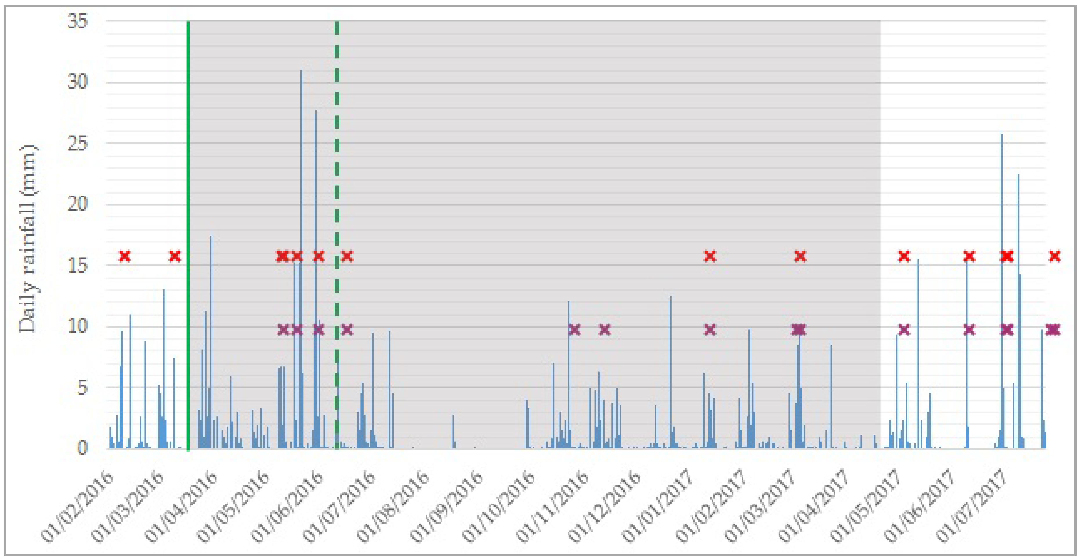
Appendix A. Daily Rainfall and Timeline of Sampled Events

Figure A1. Timeline of sampled events with daily rainfall shown in blue. Sampling events of road runoff (RR) are represented in red, while those in the BFS drain are shown in purple; note that some events sampled in close succession appear as a single mark. The mass balance period is shown in grey, the solid green line represents the installation of filter media in the biofiltration swale and the dotted green line represents installation of the check dams.
Water 11 00487 g0a1

Appendix B. Distributions Used for Stochastic Components of the Mass Balance Calculation

Table A1. Summary of distributions used to account for analytical errors.
PollutantDistribution Analytical Error
TSSNormal, μ = 0, σ = 2.9%
CuDiss: Normal, μ = 0, σ = 5%
Part: Normal, μ = 0, σ = 7%
ZnDiss: Normal, μ = 0, σ = 7%
Part: Normal, μ = 0, σ = 7%
PyrDiss: Normal, μ = 0, σ = 20%
Part: Normal, μ = 0, σ = 10%
PhenDiss: Normal, μ = 0, σ = 20%
Part: Normal, μ = 0, σ = 10%
BPADiss: Normal, μ = 0, σ = 22%
Part: Normal, μ = 0, σ = 20%
OPDiss: Normal, μ = 0, σ = 48%
Part: Normal, μ = 0, σ = 37%
NPDiss: Normal, μ = 0, σ = 29%
Part: Normal, μ = 0, σ = 34%
DEHPDiss: Normal, μ = 0, σ = 41%
Part: Normal, μ = 0, σ = 30%
Table A2. Summary of distributions used for calculating event volumes (V), TSS concentrations (CTSS) and sampled event mean concentrations (Cev) used in load calculations.
TermCaseStochastic ComponentDistribution Type and Parameters
VinAlwaysInitial lossUniform, 0.4–1 mm
VdrainMeasurement availableError VNormal, μ = 0, σ = 5%
VdrainNo measurement availableFraction of Vin drainedLog-normal, μln = −2.04, σln = 1.22
VoverMeasurement availableError hNormal, μ = 0, σ = 0.5%
VoverNo measurement availableΔVmedia,evUniform, 0–1240 L
CTSS,inTurbidity < 50 FNUCTSS,inUniform, 0–70 mg/L
CTSS,inValid turbidity measurementRegression errorNormal, μ = 0, σ = 71 mg/L
CTSS,inNo turbidity measurementCTSS,inLog-normal, μln = 5.44, σln = 0.76 mg/L
CTSS,drainWinter eventsRelationship to CTSS,inUniform, 0.225–0.883
CTSS,drainEvents outside winterCTSS,drainLog-normal, μln = 2.92, σln = 0.59 mg/L
CevSampled eventsAnalytical errorNormal, μ = 0, σ = σuncertainty, pollutant
Table A3. Summary of event mean concentration (Cev), event mean dissolved concentration (CD,ev) and event mean particle concentration (Sev) distributions used to estimate inlet concentrations for unsampled events for each pollutant. CD,ev,in and Sev,in distributions are not given for NP as turbidity was not used for this pollutant.
PollutantCev Distribution
(µg/L)
CD,ev Distribution
(µg/L)
Sev Distribution
(µg/g)
CuLog-normal μln = 5.39, σln = 0.52Log-normal μln = 5.39, σln=0.52Log-normal μln = 6.41, σln = 0.18
ZnLog-normal μln = 6.37, σln = 0.65Log-normal μln = 6.37, σln = 0.65Log-normal μln = 7.48, σln = 0.19
PyrLog-normal μln = −0.26, σln = 0.66Log-normal μln = −3.84, σln = 0.27Log-normal μln = 0.99, σln = 0.24
PhenLog-normal μln = −1.41, σln = 0.74Log-normal μln = −3.62, σln = 0.69Log-normal μln = −0.16, σln = 0.38
BPALog-normal μln = −0.77, σln = 0.41Log-normal μln = −1.21, σln = 0.59Log-normal μln = −0.75, σln = 0.52
OPLog-normal μln = −0.74, σln = 0.49Normal μln = 0.14, σln = 0.05Log-normal μln = 0.16, σln = 0.42
NPLog-normal μln = 0.52, σln = 0.48--
DEHPLog-normal μln = 2.76, σln = 0.83Log-normal μln = 1.12, σln = 0.68Log-normal μln = 3.63, σln = 0.76
Table A4. Summary of event mean concentration (Cev), event mean dissolved concentration (CD,ev) and event mean particulate concentrations (CP,ev) distributions used to estimate concentrations in drained water for each pollutant.
PollutantCev Distribution (µg/L)%Below LoQDistribution when < LoQ (µg/L)Distribution when > LoQ (µg/L)
CuLog-normal
μln = 3.65, σln = 0.94
---
ZnLog-normal
μln = 4.05, σln = 1.39
---
Pyr-CD,ev: 30%
CP,ev: 0%
CD,ev: Uniform 0–0.01CD,ev: Log-normal μln = −3.80, σln = 0.43
Part: Log-normal μln = −3.09, σln = 1.43
Phen-CD,ev: 69%
CP,ev: 15%
CD,ev: Uniform 0–0.01
CP,ev Uniform 0–0.004
CD,ev: Unform 0.012–0.098
CP,ev: Log-normal μln = −3.88, σln = 1.29
BPALog-normal
μln = −1.43, σln = 0.50
---
OPLog-normal
μln = −2.19, σln = 1.14
---
NPLog-normal
μln = −0.16, σln = 1.09
---
DEHPLog-normal
μln = 2.66, σln = 0.85
---
Table A5. Summary of distributions used for calculating masses of pollutants in the soil.
TermCaseStochastic ComponentDistribution Type and Parameters
Ssamp<LoQSsampUniform 0-LoQ
Ssamp>LoQAnalytical ErrorNormal, μ = 0, σ = σuncertainty, pollutant
fsampleZone hypothesis validZone errorZone 1: a = Uniform, −0.1–0.1
Zone 2: if a < 0: b = Uniform, (0.1-a)–0.1
else b = Uniform, −0.1-(0.1-a)
Zone 3: c = −(a + b)
fsampleZone hypothesis invalidfsampleZone 1: a = Uniform, 0–1
Zone 2: b = Uniform, 0-(1-a)
Zone 3: c = 1-a-b
f<2mmAlwaysf<2mmNormal, μ = 0.733, σ = 0.045
ρAlwaysVariability at depthUniform, −0.2–0.2
SinitAlwaysInitial composition errorNormal, μ = 0, σ = 0.139

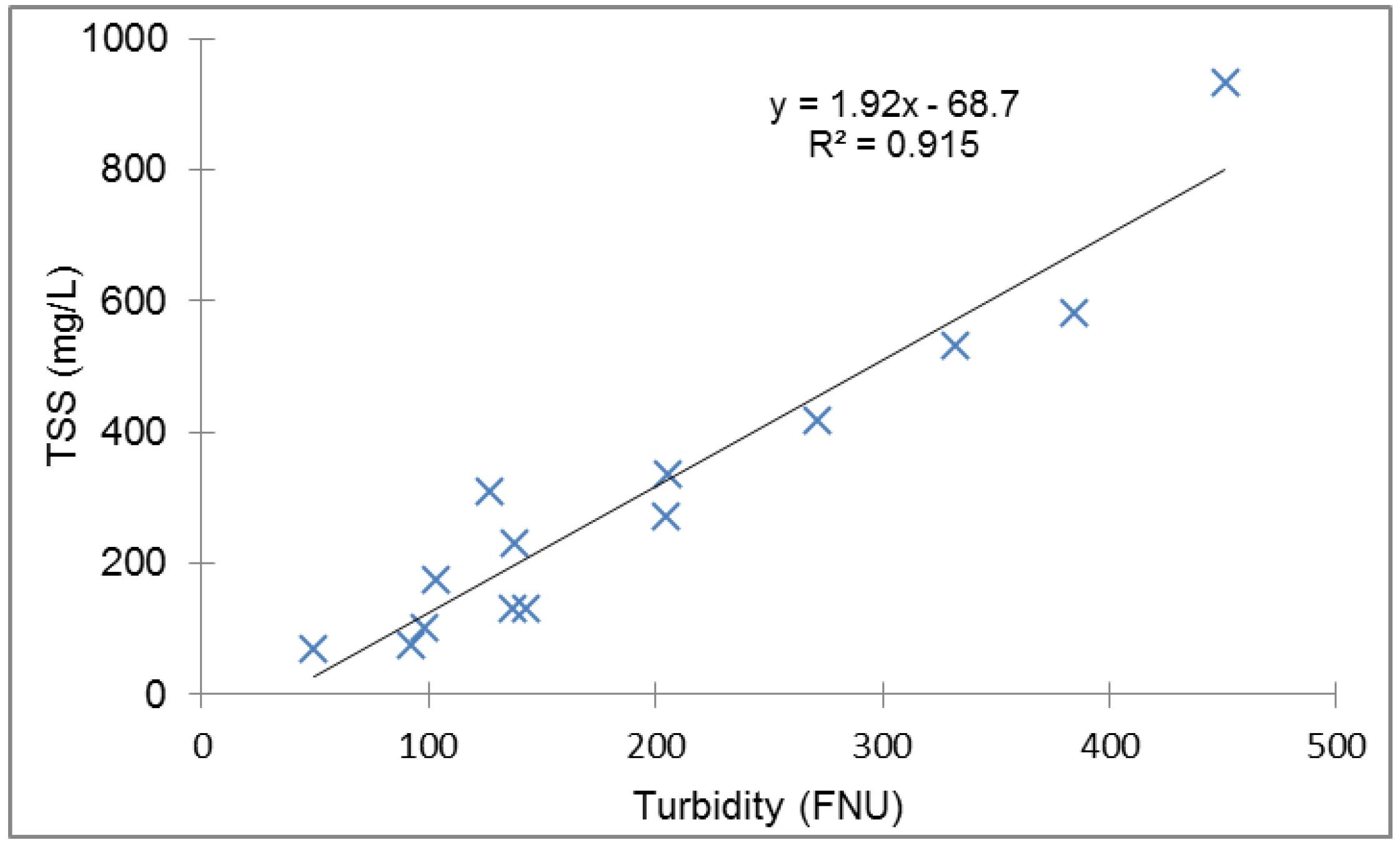
Appendix C. TSS-Turbidity Relationship

Figure A2. Event mean TSS-turbidity relationship for sampled events.
Water 11 00487 g0a2

Appendix D. Distributions of species in composite cores

The distribution of different species among composite cores may be observed in Figure A3, Figure A4, Figure A5, Figure A6, Figure A7, Figure A8 and Figure A9.
The Ca distribution (Figure A3) is mainly representative of the proportion of sand in the filter media. One may observe that calcium concentrations near the surface are closest to those observed in the initial soil sample. Samples closer to the bottom of the filter contain more calcium. This may be due to imperfections in the filter media production process, which was carried out in batches, such that different depths of the filter correspond to different batches and thus slightly different compositions.
For Cu (Figure 5a), Zn, Phen and Pyr (Figure A4, Figure A5 and Figure A6), the highest concentrations tend to be observed at the surface of each zone, as would be expected for pollutants for which the main source is infiltrating water. The one exception to this is the sample from middle depth of the C2 zone for Phen and Pyr (Figure A5 and Figure A6), which had the highest concentration despite not being at the surface. When it was constructed, a strip of asphalt was installed to guide runoff into the BFS. At the time of sampling, some of the asphalt located near the C2 zone had crumbled into the soil along the BFS. It is possible that some pieces of asphalt were included in this sample, which would explain this higher concentration, though it remains surprising that it was not located at the surface.
Distributions of BPA, OP, NP and DEHP (Figure 5b and Figure A7, Figure A8 and Figure A9) were less predictable, with higher concentrations often observed at greater depths, indicating that infiltrating water is not the only source of these pollutants. Besides the previously mentioned asphalt, other potential sources of micropollutants which may explain an accumulation of these molecules at greater depths are the geomembrane, the drain and the fabric surrounding the drain. The middle sample in the C2 zone also demonstrated high concentrations of OP, NP and DEHP, indicating that the source of PAHs present in this sample was also a source of these pollutants.
In each section (A, B and C), the only pollutants which were nearly always present at the highest concentrations in the most polluted zones from the surface cartography were Cu and Zn. Even for these pollutants, A3 was found to be slightly more contaminated than A2. This indicates that the sources, removal mechanisms or fate processes of the other pollutants differed sufficiently from those of trace metals to lead not only to different vertical distributions but also to different horizontal distributions in the soil. It also means that the choice of sampling zones was not ideal for these pollutants and that the second algorithm for calculating soil concentrations was often used.
It may also be observed that while the initial concentration of most pollutants aligns with the lowest measured concentrations in the composite cores, this was not the case for Phen and Pyr. One explanation for this is that the PAHs initially present have been partially degraded in soil. However, this hypothesis is not supported by the fact that the deficit of Pyr at the end of the study is greater than that of Phen, despite the fact that Pyr is generally less easily biodegraded (the Q20–Q80 of biodegradation half-lives range from 11–64 days for Phen and 210–1900 days for Pyr [41]). Another possible explanation is a variability in initial concentrations throughout the filter media; in this case, the initial PAH concentrations in most of the BFS may have actually been different than that in the initial soil sample. While possible variability in the initial concentration due to poor mixing top-soil and sand to produce the filter media was taken into account in the calculation, potential variations in the quality of the top-soil were not. Two composite core samples of NP presented concentrations below that in the initial soil sample. It should be noted that BPA, OP and DEHP were present at concentrations below the LoQ in the initial soil sample, so no lower concentrations could be observed.
Figure A3. Concentrations of calcium measured in composite cores of each sampling zone. Within each zone, concentrations from cores taken at depths of 0–5 cm, 5–15 cm and 15–50 cm are represented to scale from left to right. The dotted line represents the concentration measured in the initial soil sample.
Water 11 00487 g0a3
Figure A4. Concentrations of zinc measured in composite cores of each sampling zone. Within each zone, concentrations from cores taken at depths of 0–5 cm, 5–15 cm and 15–50 cm are represented to scale from left to right. The dotted line represents the concentration measured in the initial soil sample.
Water 11 00487 g0a4
Figure A5. Concentrations of phenanthrene measured in composite cores of each sampling zone. Within each zone, concentrations from cores taken at depths of 0–5 cm, 5–15 cm and 15–50 cm are represented to scale from left to right. The dotted line represents the concentration measured in the initial soil sample.
Water 11 00487 g0a5
Figure A6. Concentrations of pyrene measured in composite cores of each sampling zone. Within each zone, concentrations from cores taken at depths of 0–5 cm, 5–15 cm and 15–50 cm are represented to scale from left to right. The dotted line represents the concentration measured in the initial soil sample.
Water 11 00487 g0a6
Figure A7. Concentrations of OP measured in composite cores of each sampling zone. Within each zone, concentrations from cores taken at depths of 0–5 cm, 5–15 cm and 15–50 cm are represented to scale from left to right. The dotted line represents the concentration measured in the initial soil sample.
Water 11 00487 g0a7
Figure A8. Concentrations of NP measured in composite cores of each sampling zone. Within each zone, concentrations from cores taken at depths of 0–5 cm, 5–15 cm and 15–50 cm are represented to scale from left to right. The dotted line represents the concentration measured in the initial soil sample.
Water 11 00487 g0a8
Figure A9. Concentrations of DEHP measured in composite cores of each sampling zone. Within each zone, concentrations from cores taken at depths of 0–5 cm, 5–15 cm and 15–50 cm are represented to scale from left to right. The dotted line represents the concentration measured in the initial soil sample.
Water 11 00487 g0a9

Appendix E. All Mass Balance Terms

Table A6. Summary of all mass balance terms. Individual mass balance terms associated with water fluxes (inlet mass from road runoff–Min, outlet mass from drain–Mout,drain, outlet mass from overflow–Mout,over) and soil (initial mass stored in soil–Msoil,initial, final mass stored in soil–Msoil,final).
PollutantMin (g)Mout,drain (g)Mout,over (g)Msoil,initial (g)Msoil,final (g)
TSS43,200
(36,800, 57,600)
5500
(4540, 6900)
8420
(5180, 18,800)
--
OC7320
(6320, 8970)
1220
(1900, 1620)
1080
(2820, 4200)
86,700
(75,100, 100,000)
52,200
(46,600, 58,700)
Cu32.5
(28.2, 39.8)
4.53
(3.51, 6.41)
7.40
(4.96, 12.7)
126
(110, 143)
151
(138, 164)
Zn90.0
(76.1, 118)
11.4
(7.99, 21.0)
19.1
(11.8, 40.2)
313
(271, 362)
432
(394, 471)
Pyr0.125
(0.106, 0.162)
0.00838
(0.0060, 0.0155)
0.0256
(0.0157, 0.0536)
1.45
(1.09, 1.85)
1.11
(0.830, 1.48)
Phen0.0439
(0.0366, 0.0586)
0.00295
(0.00218, 0.00464)
0.00992
(0.00650, 0.0211)
0.718
(0.541, 0.920)
0.824
(0.610, 1.12)
BPA0.0797
(0.0693, 0.0934)
0.0208
(0.0180, 0.0252)
0.0230
(0.0172, 0.0322)
0.0525
(0.0180, 0.0893)
0.349
(0.267, 0.503)
OP0.0821
(0.0697, 0.0983)
0.0168
(0.0118, 0.0267)
0.0214
(0.0149, 0.0322)
0.0333
(0.0117, 0.0562)
0.241
(0.141, 0.411)
NP0.301
(0.257, 0.360)
0.106
(0.0766, 0.168)
0.0846
(0.0599, 0.125)
1.58
(1.04, 2.16)
3.08
(2.31, 4.06)
DEHP2.95
(2.31, 4.17)
1.50
(1.15, 2.08)
0.606
(0.357, 1.50)
5.56
(2.98, 8.34)
26.4
(15.1, 44.3)
Table A7. Net mass balance terms associated with water fluxes (difference between mass entering and exiting the system–Mintercepted) and soil (difference between initial and final masses stored in soil–ΔMsoil).
PollutantMintercepted (g)ΔMsoil (g)
TSS29,000
(24,900, 35,300)
-
OC4200
(3430, 5060)
−34,500
(−46,500, −23,700)
Cu20.5 (17.2, 24.1)24.8 (10.3, 39.2)
Zn58.8 (46.6, 72.0)119 (73.5, 162)
Pyr0.0901 (0.0755, 0.108)−0.337 (−0.824, 0.160)
Phen0.0307 (0.0255, 0.0377)0.107 (−0.180, 0.437)
BPA0.0355 (0.0277, 0.0442)0.297 (0.207, 0.452)
OP0.0434 (0.0308, 0.0549)0.208 (0.106, (0.377)
NP0.108 (0.0422, 0.156)1.51 (0.589, 2.60)
DEHP0.806 (0.063, 1.58)20.9 (9.01, 38.9)

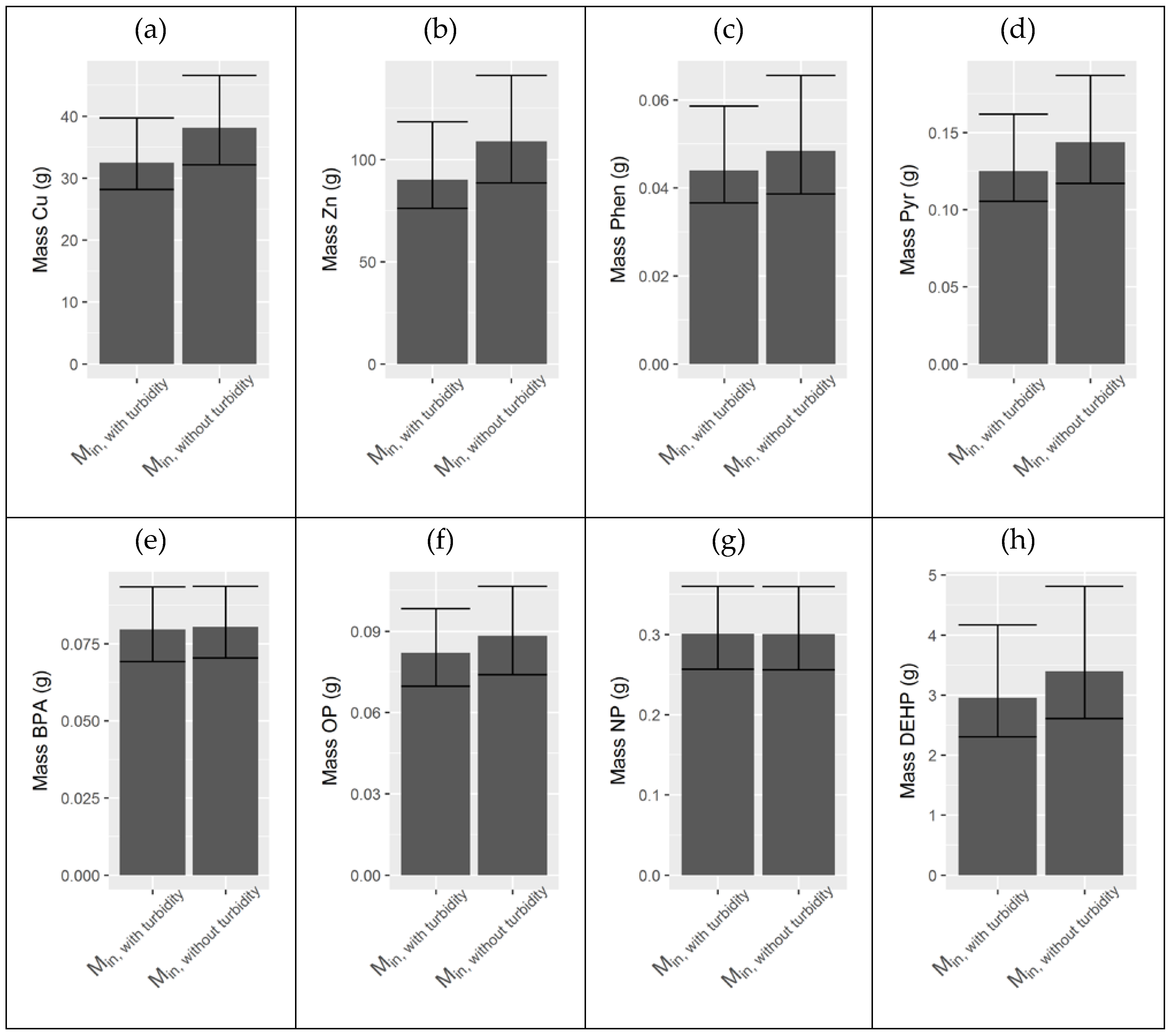
Appendix F. Comparison of Inlet Masses with and without Turbidity Data

Figure A10 shows the difference between inlet masses calculated with and without turbidity data. The use of turbidity tends to slightly decrease uncertainties, reducing the confidence interval, for example from (−15, 23%) to (−13, 22%) for copper. In addition, masses calculated using turbidity data were lower than those evaluated without turbidity data. This is likely due to the fact that the distribution of event mean turbidity measurements for sampled events were slightly higher than those of the full period. This indicates that particulate concentrations and total concentrations of mainly particulate pollutants, were also likely higher for sampled events than for the full period. The use of turbidity data allows for the correction of this bias.
As turbidity improves estimations of particulate concentrations and mass, it does little to change masses calculated for more dissolved pollutants, like BPA (Figure A10e). There is no change in inlet mass calculations with and without turbidity data for NP, as particulate concentrations were not correlated with TSS concentrations; therefore, turbidity was never used in the algorithm for calculating NP input mass.
Figure A10. Comparison of inlet mass calculations with and without turbidity data for (a) copper, (b) zinc, (c) phenanthrene, (d) pyrene, (e) bisphenol-A, (f) octylphenol, (g) nonylphenol and (h) bis(2-ethylhexyl) phthalate. Bars represent medians, while error bars represent the 95% confidence interval.
Water 11 00487 g0a10

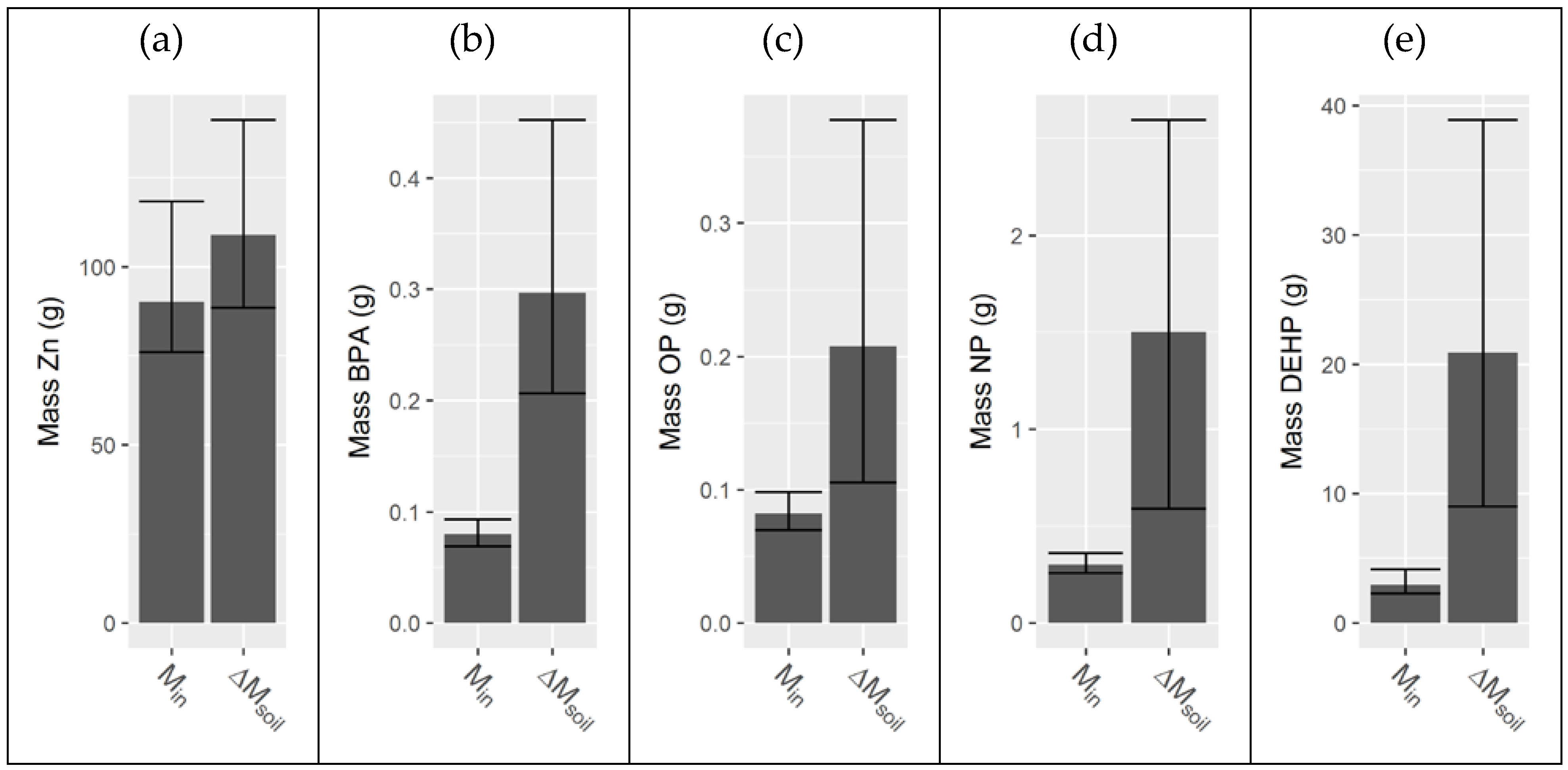
Appendix G. Comparison on Inlet Mass to Mass Accumulated in the Soil

Figure A11. Comparison of inlet mass (Min) to the change in soil mass over time (ΔMsoil) for (a) zinc, (b) bisphenol-A, (c) octylphenol, (d) nonylphenol and (e) bis(2-ethylhexyl) phthalate. Bars represent medians, while error bars represent the 95% confidence interval.
Water 11 00487 g0a11

Appendix H. Contamination of Atmospheric Deposition

Atmospheric deposition was not characterized in the present field study. However, atmospheric deposition washed off by rainfall was collected using a stainless steel pyramid funnel at a distance of about 10 m from the road side as a part of a parallel study of the same site by the public authority which constructed and operates the BFS site [36]. It was analysed for some of the same pollutants studied in the present work (Cu, Zn, Phen and Pyr). These results (Table A5) show that concentrations of all pollutants characterized in total fallout are at least an order of magnitude below those observed in road runoff. Atmospheric deposition data is unavailable for BPA, OP, NP and DEHP.
Table A8. Concentrations observed in road runoff in the present study compared to those due to atmospheric deposition. Median, minimum and maximum observed values are presented. 1 Data from [36].
Road RunoffAtmospheric Deposition 1
Cu (µg/L)258 (98.1, 547)3.9 (1.9, 22)
Zn (µg/L)693 (236, 1650)38 (18, 105)
Phen (µg/L)0.356 (0.102, 0.594)0.014 (<0.01, 0.036)
Pyr (µg/L)0.851 (0.205, 2.30)0.0085 (0.005, 0.035)

Appendix I. Galvanized Steel Barrier along the Biofiltration Swale

Figure A12. Galvanized steel safety barrier separating the biofiltration swale from the road surface.
Water 11 00487 g0a12

Appendix J. Proportion of Intercepted Pollutant Mass Dissipated in the System (Esoil) and Relative Uncertainty Values

Table A9. Percent difference between the change in pollutant mass recovered in the system at the end of the period compared to the mass of pollutant intercepted (Esoil) for all pollutants. Median and 95% confidence interval are presented.
PollutantEsoil (%)
Pyr474 (−76, 1039)
Phen−242 (−1350, 682)
BPA−739 (−1270, −447)
OP−383 (−852, −133)
NP−1310 (−3610, −410)
DEHP−2520 (−13300, −789)

Appendix K. Relative Uncertainty Values

Table A10. Relative uncertainties (95% confidence interval) for all terms micropollutants, in percentage.
Msoil,initialMsoil,finalΔMsoilMinMout,drainMout,overMinterceptedEsoil
Cu[−12,14][−8,9][−14,11][−13,22][−23,41][−33,71][−16,18]-
Zn[−14,16][−9,9][−38,37][−15,32][−30,85][−38,110][−21,22]-
Pyr[−25,27][−25,33][−145,147][−16,30][−29,85][−39,113][−16,20][−116,119]
Phen[−25,28][−26,35][−269,310][−17,33][−26,57][−34,113][−17,23][−457,382]
BPA[−66,70][−23,44][−30,52][−13,17][−13,21][−25,40][−22,25][−72,40]
OP[−65,69][−41,71][−49,82][−15,20][−29,59][−30,51][−29,26][−123,65]
NP[−34,37][−25,32][−61,73][−15,20][−28,58][−29,47][−61,44][−175,69]
DEHP[−46,50][−43,68][−57,86][−22,41][−36,39][−41,148][−92,95][−427,69]

References

  1. Fletcher, T.D.; Shuster, W.; Hunt, W.F.; Ashley, R.; Butler, D.; Arthur, S.; Trowsdale, S.; Barraud, S.; Semadeni-Davies, A.; Bertrand-Krajewski, J.-L.; et al. SUDS, LID, BMPs, WSUD and more—The evolution and application of terminology surrounding urban drainage. Urban Water J. 2014, 12, 525–542. [Google Scholar] [CrossRef]
  2. EC Directive 2013/39/EU of the European Parliament and of the Council of 12 August 2013 amending Directives 2000/60/EC and 2008/105/EC as regards priority substances in the Field of Water Policy 2013. Available online: https://eur-lex.europa.eu/%20LexUriServ/LexUriServ.do?uri=OJ:L:2013:226:0001:0017:EN:PDF (accessed on 30 March 2018).
  3. Davis, A.P.; Hunt, W.F.; Traver, R.G.; Clar, M. Bioretention technology: Overview of current practice and future needs. J. Environ. Eng. 2009, 135, 109–117. [Google Scholar] [CrossRef]
  4. Roy-Poirier, A.; Champagne, P.; Filion, Y. Review of bioretention system research and design: Past, present, and future. J. Environ. Eng. 2010, 136, 878–889. [Google Scholar] [CrossRef]
  5. LeFevre, G.; Paus, K.H.; Natarajan, P.; Gulliver, J.S.; Novak, P.J.; Hozalski, R.M. Review of Dissolved Pollutants in Urban Storm Water and Their Removal and Fate in Bioretention Cells. J. Environ. Eng. 2014, 141. [Google Scholar] [CrossRef]
  6. Davis, A.P. Field Performance of Bioretention: Water Quality. Environ. Eng. Sci. 2007, 24, 1048–1064. [Google Scholar] [CrossRef]
  7. DiBlasi, C.J.; Li, H.; Davis, A.P.; Ghosh, U. Removal and Fate of Polycyclic Aromatic Hydrocarbon Pollutants in an Urban Stormwater Bioretention Facility. Environ. Sci. Technol. 2009, 43, 494–502. [Google Scholar] [CrossRef] [PubMed]
  8. Dietz, M.E.; Clausen, J.C. A field evaluation of rain garden flow and pollutant treatment. Water. Air. Soil Pollut. 2005, 167, 123–138. [Google Scholar] [CrossRef]
  9. Hatt, B.; Fletcher, T.D.; Deletic, A. Hydrologic and pollutant removal performance of stormwater biofiltration systems at the field scale. J. Hydrol. 2009, 365, 310–321. [Google Scholar] [CrossRef]
  10. Hunt, W.F.; Jarrett, A.R.; Smith, J.T.; Sharkey, L.J. Evaluating Bioretention Hydrology and Nutrient Removal at Three Field Sites in North Carolina. J. Irrig. Drain. Eng. 2006, 132, 600–608. [Google Scholar] [CrossRef] [Green Version]
  11. Monrabal-Martinez, C.; Meyn, T.; Muthanna, T.M. Characterization and temporal variation of urban runoff in a cold climate—Design implications for SuDS. Urban Water J. 2018, 1–9. [Google Scholar] [CrossRef]
  12. Flanagan, K.; Branchu, P.; Boudahmane, L.; Caupos, E.; Demare, D.; Deshayes, S.; Dubois, P.; Meffray, L.; Partibane, C.; Saad, M.; et al. Retention and transport processes of particulate and dissolved micropollutants in stormwater biofilters treating road runoff. Sci. Total Environ. 2019, 656, 1178–1190. [Google Scholar] [CrossRef] [PubMed]
  13. Tedoldi, D.; Chebbo, G.; Pierlot, D.; Kovacs, Y.; Gromaire, M.-C. Impact of runoff infiltration on contaminant accumulation and transport in the soil/filter media of Sustainable Urban Drainage Systems: A literature review. Sci. Total Environ. 2016, 569, 904–926. [Google Scholar] [CrossRef] [PubMed]
  14. Hong, E.; Seagren, E.A.; Davis, A.P. Sustainable Oil and Grease Removal from Synthetic Stormwater Runoff Using Bench-Scale Bioretention Studies. Water Environ. Res. 2006, 78, 141–155. [Google Scholar] [CrossRef] [PubMed] [Green Version]
  15. LeFevre, G.H.; Novak, P.J.; Hozalski, R.M. Fate of Naphthalene in Laboratory-Scale Bioretention Cells: Implications for Sustainable Stormwater Management. Environ. Sci. Technol. 2012, 46, 995–1002. [Google Scholar] [CrossRef] [PubMed]
  16. Leroy, M.C.; Legras, M.; Marcotte, S.; Moncond’huy, V.; Machour, N.; Le Derf, F.; Portet-Koltalo, F. Assessment of PAH dissipation processes in large-scale outdoor mesocosms simulating vegetated road-side swales. Sci. Total Environ. 2015, 520, 146–153. [Google Scholar] [CrossRef] [PubMed]
  17. LeFevre, G.H.; Hozalski, R.M.; Novak, P.J. The role of biodegradation in limiting the accumulation of petroleum hydrocarbons in raingarden soils. Water Res. 2012, 46, 6753–6762. [Google Scholar] [CrossRef] [PubMed]
  18. Maniquiz, M.C.; Kim, L.-H.; Lee, S.; Choi, J. Flow and mass balance analysis of eco-bio infiltration system. Front. Environ. Sci. Eng. 2012, 6, 612–619. [Google Scholar] [CrossRef]
  19. Johnston, C.A. Development and Evaluation of Infilling Methods for Missing Hydrologic and Chemical Watershed Monitoring Data. Master’s Thesis, Virginia Polytechnic Institute and State University, Blacksburg, VA, USA, 1999. [Google Scholar]
  20. Sun, S.; Barraud, S.; Castebrunet, H.; Aubin, J.-B.; Marmonier, P. Long-term stormwater quantity and quality analysis using continuous measurements in a French urban catchment. Water Res. 2015, 85, 432–442. [Google Scholar] [CrossRef] [PubMed]
  21. Bertrand-Krajewski, J.-L.; Bardin, J.-P.; Mourad, M.; Béranger, Y. Accounting for sensor calibration, concentration heterogeneity, measurement and sampling uncertainties in monitoring urban drainage systems. Water Sci. Technol. 2003, 47, 95–102. [Google Scholar] [CrossRef] [PubMed]
  22. Versini, P.-A.; Joannis, C.; Chebbo, G. Guide technique sur la mesurage de la turbidité dans les réseaux d’assainissement; Onema: Vincennes, France, 2015. [Google Scholar]
  23. Flanagan, K.; Branchu, P.; Boudahmane, L.; Caupos, E.; Demare, D.; Deshayes, S.; Dubois, P.; Meffray, L.; Partibane, C.; Saad, M.; et al. Field performance of two biofiltration systems treating micropollutants from road runoff. Water Res. 2018, 145, 562–578. [Google Scholar] [CrossRef] [PubMed]
  24. Tedoldi, D.; Chebbo, G.; Pierlot, D.; Kovacs, Y.; Gromaire, M.-C. Assessment of metal and PAH profiles in SUDS soil based on an improved experimental procedure. J. Environ. Manag. 2017, 202, 151–166. [Google Scholar] [CrossRef] [PubMed] [Green Version]
  25. Sage, J. Concevoir et optimiser la gestion hydrologique du ruissellement pour une maîtrise à la source de la contamination des eaux pluviales urbaines. Ph.D. Thesis, Université de Paris-Est, Champs-sur-Marne, France, 2016. [Google Scholar]
  26. Hollis, G.E.; Ovenden, J.C. One year irrigation experiment to assess losses and runoff volume relationships for a residential road in hertfordshire, England. Hydrol. Process. 1988, 2, 61–74. [Google Scholar] [CrossRef]
  27. Ramier, D.; Berthier, E.; Andrieu, H. The hydrological behaviour of urban streets: Long-term observations and modelling of runoff losses and rainfall-runoff transformation. Hydrol. Process. 2011, 25, 2161–2178. [Google Scholar] [CrossRef]
  28. Hannouche, A.; Chebbo, G.; Joannis, C.; Gasperi, J.; Gromaire, M.-C.; Moilleron, R.; Barraud, S.; Ruban, V. Stochastic evaluation of annual micropollutant loads and their uncertainties in separate storm sewers. Environ. Sci. Pollut. Res. 2017, 24, 28205–28219. [Google Scholar] [CrossRef] [PubMed]
  29. Van Buren, M.A.; Watt, W.E.; Marsalek, J. Application of the log-normal and normal distributions to stormwater quality parameters. Water Res. 1997, 31, 95–104. [Google Scholar] [CrossRef]
  30. Bertrand-Krajewski, J.-L.; Chebbo, G.; Saget, A. Distribution of pollutant mass vs volume in stormwater discharges and the first flush phenomenon. Water Res. 1998, 32, 2341–2356. [Google Scholar] [CrossRef]
  31. Huber, M.; Helmreich, B. Stormwater Management: Calculation of Traffic Area Runoff Loads and Traffic Related Emissions. Water 2016, 8, 294. [Google Scholar] [CrossRef]
  32. Björklund, K.; Cousins, A.P.; Strömvall, A.-M.; Malmqvist, P.-A. Phthalates and nonylphenols in urban runoff: Occurrence, distribution and area emission factors. Sci. Total Environ. 2009, 407, 4665–4672. [Google Scholar] [CrossRef] [PubMed]
  33. Bressy, A.; Gromaire, M.-C.; Lorgeoux, C.; Saad, M.; Leroy, F.; Chebbo, G. Towards the determination of an optimal scale for stormwater quality management: Micropollutants in a small residential catchment. Water Res. 2012, 46, 6799–6810. [Google Scholar] [CrossRef]
  34. Lamprea, K.; Bressy, A.; Mirande-Bret, C.; Caupos, E.; Gromaire, M.-C. Alkylphenol and bisphenol A contamination of urban runoff: An evaluation of the emission potentials of various construction materials and automotive supplies. Environ. Sci. Pollut. Res. 2018, 25, 21887–21900. [Google Scholar] [CrossRef]
  35. Hatt, B.; Morison, P.; Fletcher, T.; Deletic, A. Stormwater Biofiltration Systems: Adoption Guidelines; Monash University: Clayton, Victoria, Australia, 2009. [Google Scholar]
  36. Thomas, E.; Ratovelomanana, T. RD 212: Expérimentation d’un Assainissement Alternatif Routier; CD 77: Vert-Saint-Denis, France, 2016. [Google Scholar]
  37. Bergé, A.; Cladière, M.; Gasperi, J.; Coursimault, A.; Tassin, B.; Moilleron, R. Meta-analysis of environmental contamination by alkylphenols. Environ. Sci. Pollut. Res. 2012, 19, 3798–3819. [Google Scholar] [CrossRef] [PubMed]
  38. Markiewicz, A.; Björklund, K.; Eriksson, E.; Kalmykova, Y.; Strömvall, A.-M.; Siopi, A. Emissions of organic pollutants from traffic and roads: Priority pollutants selection and substance flow analysis. Sci. Total Environ. 2017, 580, 1162–1174. [Google Scholar] [CrossRef]
  39. Taylor, J.R. An Introduction to Error Analysis, 2nd ed.; University Science Books: Sausalito, CA, USA, 1997. [Google Scholar]
  40. Gaspéri, J.; Ayrault, S.; Moreau-Guigon, E.; Alliot, F.; Labadie, P.; Budzinski, H.; Blanchard, M.; Muresan, B.; Caupos, E.; Cladière, M.; et al. Contamination of soils by metals and organic micropollutants: Case study of the Parisian conurbation. Environ. Sci. Pollut. Res. 2016. [Google Scholar] [CrossRef]
  41. Mackay, D. (Ed.) Handbook of Physical-Chemical Properties and Environmental Fate for Organic Chemicals, 2nd ed.; CRC/Taylor & Francis: Boca Raton, FL, USA, 2006; ISBN 978-1-56670-687-2. [Google Scholar]
Figure 1. The Compans experimental site.
Water 11 00487 g001
Figure 2. Schematic of (a) surface soil sampling and (b) core sampling of the biofiltration swale in Compans. Surface samples were taken at each blue x (a), while cores were taken at each orange circle and mixed according to zones (A1, A2, A3, B1, B2, B3 and C1, C2) selected based on the cartography of copper concentrations shown in the background (b). Please note that horizontal and vertical scales are different.
Water 11 00487 g002
Figure 3. Generalized method for evaluating flow volumes in and out of the biofilter.
Water 11 00487 g003
Figure 4. Generalized method for evaluating concentrations associated with each flow term.
Water 11 00487 g004
Figure 5. Concentrations of (a) copper and (b) bisphenol-A (BPA) measured in composite cores of each sampling zone. Within each zone, concentrations from cores taken at depths of 0–5 cm, 5–15 cm and 15–50 cm are represented to scale from left to right. The dotted line represents the concentration measured in the initial soil sample.
Water 11 00487 g005
Figure 6. Method for selecting soil mass associated with each sample and each pollutant.
Water 11 00487 g006
Figure 7. Method for estimating initial soil concentration for each pollutant.
Water 11 00487 g007
Figure 8. Individual mass balance terms associated with water fluxes (inlet mass from road runoff–Min, outlet mass from drain–Mout,drain, outlet mass from overflow–Mout,over) and soil (initial mass stored in soil–Msoil,initial, final mass stored in soil–Msoil,final) for (a) copper, (b) zinc, (c) phenanthrene, (d) pyrene, (e) bisphenol-A, (f) octylphenol, (g) nonylphenol and (h) bis(2-ethylhexyl) phthalate. Bars represent medians, while error bars represent the 95% confidence interval.
Water 11 00487 g008
Figure 9. Net mass balance terms associated with water fluxes (difference between mass entering and exiting the system–Mintercepted) and soil (difference between initial and final masses stored in soil–ΔMsoil) for (a) copper, (b) zinc, (c) phenanthrene, (d) pyrene, (e) bisphenol-A, (f) octylphenol, (g) nonylphenol and (h) bis(2-ethylhexyl) phthalate. Bars represent medians, while error bars represent the 95% confidence interval.
Water 11 00487 g009
Table 1. Filter media and geometric properties of the biofiltration swale.
PropertiesBiofiltration Swale
Filter media textureSandy loam
Filter media pH in water8.73
Initial organic carbon content (by mass, %)0.9
Hydraulic conductivity (mm/h)21
Filter media depth (cm)50
Ponding depth (cm)17
Width (perpendicular to road, m)0.5
Length (parallel to road, m)32
Surface area ratio (Adevice/Acatchment, %)4.5
Table 2. Summary of employed analytical methods. M is the mass of TSS extracted in mg, which varied according to the concentration of TSS in the water sample and the filtered volume. Abbreviations: ICP-OES (inductively coupled plasma optical emission spectroscopy), ICP-MS (inductively coupled plasma mass spectrometry), GC-MS (gas chromatography coupled with mass spectrometry), UPLC-MSMS (ultra performance liquid chromatography with tandem mass spectrometry).
ParameterSubstances and AbbreviationsMethodLimit of Quantification (LoQ)Uncertainty
Suspended solidsTotal suspended solids (TSS)Filter: 0.7 µm fiberglass
Method: Filtration
Standard: NF EN 872
2 mg/L ± 10 3
Organic carbonOrganic carbon (OC)Filter: 0.7 µm fiberglass
Method: Thermal combustion-Infrared detector
Standard: NF EN 1484 (dissolved)
Dissolved:
0.3 mg/L
Particulate:
70 M mg/g
±10%
Trace metalsCopper (Cu), Zinc (Zn)Filter: 0.45 µm cellulose acetate
Methods: ICP-MS and ICP-OES
Extraction: Total solubilization by HF and HClO4 acid digestion, evaporation and resuspension with HNO3 (particulate)
Standards: NF X31-147 (acid digestion), NF EN ISO 17294 (ICP-MS), NF EN ISO 11885 (ICP-OES)
Dissolved:
0.2 (Cu), 0.3 (Zn) µg/L
Particulate: 0.4 (Cu), 1 (Zn) mg/kg
Dissolved:
±9 (Cu), 14 (Zn) %
Particulate: ± 14 (Cu), 13 (Zn) %
PAHsPhenanthrene (Phen), Pyrene (Pyr)Filter: 0.7 µm fiberglass
Extraction: Liquid-liquid (dissolved), ultrasound solid-liquid (particulate)
Method: GC-MSStandard: XP ISO-TS 28581 and NF ISO 28540 (dissolved), XP X33-012 and NF EN 15527 (particulate)
Dissolved:
10 ng/L
Particulate:
20 M µg/g
SL: 20 ng/L (dissolved), 0.03 µg/g (particulate)
Absolute uncertainty between LoQ and SL: ± 6 ng/L (dissolved), 0.006 µg/g (particulate)
Relative uncertainty beyond SL: ± 40 (dissolved), 20 (particulate) %
BPA/APBisphenol-A (BPA), Para-nonylphenol (NP), 4-tert-octylphenol (OP)Filter: 0.7 µm fiberglass
Extraction: Solid-phase (dissolved), Microwave (particulate)
Method: UPLC-MSMS
Dissolved:
11 (BPA), 79 (NP), 7 (OP) ng/L
Particulate:
2.6 M (BPA), 20 M (NP), 1.7 M (OP) µg/g
Dissolved: ± 28 (BPA), 37 (NP), 61 (OP) %
Particulate: ± 25 (BPA), 44 (NP), 48 (OP) %
PhthalatesBis(2-ethylhexyl) phthalate (DEHP)Filter: 0.7 µm fiberglass
Extraction: Solid-phase (dissolved), Microwave (particulate)
Method: GC-MS
Dissolved:
350 (DEHP) ng/L
Particulate:
88 M (DEHP) µg/g
Dissolved: ± 53 (DEHP) %
Particulate: ± 35 (DEHP) %
Table 3. Summary of pollutant loads in road runoff, median and 95% confidence interval.
PollutantMin over Full Period (g)Min (g/ha/year)Min (mg/ act.ha/mm)
TSS4.3 × 104 (3.7 × 10⁴, 5.8 × 10⁴)1.1 × 10⁶ (9.6 × 10⁵, 1.5 × 10⁶)2.7 × 10⁶ (2.3 × 10⁶, 3.5 × 10⁶)
OC7.3 × 103 (6.3 × 10³, 9.0 × 10³)1.9 × 10⁵ (1.7 × 10⁵, 2.4 × 10⁵)4.5 × 10⁵ (4.0 × 10⁵, 5.5 × 10⁵)
Cu32.5 (28.2, 39.8)851 (738, 1040)2010 (1740, 2450)
Zn90.1 (76.1, 118)2360 (1990, 3100)5560 (4770, 7300)
Pyr0.125 (0.106, 0.162)3.27 (2.76, 4.24)7.71 (6.51, 10.0)
Phen0.0439 (0.0366, 0.0586)1.15 (0.96, 1.53)2.71 (2.26, 3.61)
BPA0.0797 (0.0693, 0.934)2.09 (1.81, 2.45)4.92 (4.27, 5.76)
OP0.0821 (0.0697, 0.0983)2.15 (1.83, 2.57)5.06 (4.30, 6.07)
NP0.300 (0.257, 0.360)7.87 (6.73, 9.43)18.6 (15.9, 22.2)
DEHP2.95 (2.31, 4.17)77.3 (60.4, 109.3)182 (142, 257)
Table 4. Summary of water volume and pollutant mass reduction Eint, proportions of inlet volume and loads accounted for in overflow (Mout,over/Min) and in drained water (Mout,drain/Min) and event mean concentration reductions (Ec 1 see [23] for more details), median and 95% confidence interval.
ParameterEint (%)Mout,over/Min (%)Mout,drain/Min (%)Ec (%) 1
Volume21 (15, 24)35 (31, 37)45 (41, 52)-
TSS67 (56, 74)20 (13, 34)13 (9, 16)92 (27, 95)
OC57 (48, 64)22 (16, 32)20 (15, 27)70 (25, 77)
Cu63 (54, 69)23 (17, 33)14 (10, 20)76 (29, 92)
Zn65 (51, 73)21 (15, 34)13 (8, 24)89 (35, 97)
Pyr72 (60, 79)21 (14, 34)7 (4, 13)94 (49, 95)
Phen70 (58, 77)23 (16, 37)7 (4, 11)92 (43, 95)
BPA45 (38, 51)29 (23, 36)26 (21, 33)57 (−44, 77)
OP53 (40, 62)26 (20, 34)20 (14, 33)76 (−77, 93)
NP36 (15, 48)28 (22, 36)35 (24, 57)56 (−214, 71)
DEHP27 (3, 44)21 (13, 38)51 (33, 77)9 (−128, 32)

