Comparative Study of Regional Frequency Analysis and Traditional At-Site Hydrological Frequency Analysis

State Key Laboratory of Hydraulic and Mountain River Engineering, College of Water Resources and Hydropower, Sichuan University, Chengdu 610065, China
*
Authors to whom correspondence should be addressed.
Water 2019, 11(3), 486; https://doi.org/10.3390/w11030486
Submission received: 1 February 2019
/
Revised: 4 March 2019
/
Accepted: 4 March 2019
/
Published: 7 March 2019
(This article belongs to the Special Issue Flood Modelling: Regional Flood Estimation and GIS Based Techniques)
Abstract
:Hydrological frequency analysis plays an indispensable role in the construction of national flood control projects. This study selects the stations with the smallest and largest discordances in the nine homogeneous regions of Sichuan Province as the representative stations, and results obtained by regional frequency analysis are compared with those obtained by traditional at-site hydrological frequency analysis. The results showed that the optimal frequency distribution of each representative station obtained by traditional at-site hydrological frequency analysis and the ones of corresponding homogeneous regions obtained by regional frequency analysis were not necessarily consistent, which was related to the site and homogeneous regions. At the same time, there were also differences between the fitting of the theoretical rainstorm frequency curve obtained by the two methods and the observation. In general, in each homogeneous region, the results obtained by regional frequency analysis and traditional at-site hydrological frequency analysis at the stations with the largest frequency analysis were quite different. The design values obtained by the two methods were also increasingly different with the increase of the return period. The study has specific reflections on the differences between regional frequency analysis and traditional at-site hydrological frequency analysis.
1. Introduction
Natural disasters cause serious losses to society and the economy, and the occurrence of flood disasters has the greatest impact on society [1]. Hydrological frequency analysis is a scientific criterion for assessing natural disasters, especially water disasters caused by extreme hydrological events [2]. Hydrological frequency analysis is one of the main ways to ensure the reliability of flood control construction [3]. Hydrological frequency analysis takes hydrological elements as random events, and its change law obeys the probability distribution law. Therefore, probability theory and mathematical statistics methods are used to make “probability estimations” for future hydrological situations, so as to obtain hydrological design values under different return periods. The hydrological design value obtained by a hydrological frequency analysis of flood data or flow data can provide a safety standard for the construction of flood control projects [4]. However, due to the limited flood data or flow data in actual projects, the use of rainfall data to indirectly design floods has become a necessary method. Precipitation in China is extremely uneven in time scale and spatial scale, with obvious seasonal and regional changes and inter-annual differences [5], which has frequently caused floods in China. Therefore, research on rainfall is of great significance to the construction of flood control work in China to a certain extent [6]. For a long time, the methods of a hydrological frequency analysis in various countries mainly considered the selection of single distributions to analyze the data of a single station, until a new hydrological frequency analysis method—regional frequency analysis—was proposed and received extensive research. Traditional at-site hydrological frequency analysis requires longer sequences to obtain more reliable design values [7]. Regional frequency analysis reduces the requirements for hydrological data to a certain extent. It has been proven that regional frequency analysis is also suitable for hydrological frequency analysis when the length of the site data sequence is short or difficult to obtain [8]. This is because the application of regional analysis in hydrological frequency analysis can effectively extend the hydrological information between stations in the same homogeneous region [9]. It is well-accepted that regional frequency analysis based on L-moments has more accuracy and reliability than the traditional hydrological frequency analysis method [10]. Regional frequency analysis has been fully applied to the flood control works, and the quantiles estimated by regional frequency analysis have been also set as the national standard for flood control in the United States in 2006 [11]. So far, foreign scholars still have more in depth research on regional frequency analysis. Haddad et al. [12] proposed an approach using Bayesian generalized least squares regression in a region-of-influence framework for regional flood frequency analysis of the data from 399 catchments in eastern Australia. Durocher et al. [13] took a database of 771 sites across Canada as an example and validated successful settings to carry out regional frequency analysis using the regions of influence(ROI)/the generalized least squares(GLS) framework. Abdi et al. [14] proposed two new methods for increasing the accuracy of the multivariate regional frequency analysis, the two methods were the optimization-based method (OBM) and the rank-based method (RBM). However, the application of regional frequency analysis in China is still relatively less than other countries.
There are a number of research studies on regional frequency analysis in China. Chen et al. [15] analyzed the annual maximum flood sequence of five hydrological stations in the middle and lower reaches of the Yangtze river by using regional frequency analysis. It was believed that the five sites could be considered a homogeneous region of hydrological frequency analysis, and the regional distribution was a Wakeby distribution. Wu et al. [16] used regional frequency analysis to analyze the rainstorm frequency in the Taihu Basin, and considered that the southwest mountainous area was a high-risk area for heavy rainfall in the Taihu Basin. Shao et al. [17] divided the Huaihe River into six homogeneous regions based on regional frequency analysis, and obtained the optimal distribution of each homogeneous region. Xiong et al. [18] summarized the progress of foreign research on regional frequency analysis. Li et al. [19] proposed a simple and easy-to-operate correction method based on spatial round-trip quadratic interpolation to solve the spatial discontinuity of storm design values in homogeneous regions obtained by regional frequency analysis. Liang et al. [20] made a comparative study of rainfall frequency analysis in Taihu Lake Basin by using the L-moment method and conventional moments method. The results showed that the accuracy, unbiasedness, and robustness of the parameters were better than the conventional moment method when estimating the parameters by L-moment. Hassan et al. [21] selected 17 sites in the Weihe River Basin of Hebei Province, China, divided 17 sites in the Weihe River Basin into four homogeneous regions, and determined the frequency distribution of each homogeneous region. Liang et al. [22] conducted comparative studies on the uncertainty of L-moment-based regional frequency analysis and at-site hydrological frequency analysis and believed that L-moment-based regional frequency analysis was more robust and accurate than at-site hydrological analysis. Yang et al. [23] used the L-moment method and the highest measured flood level of 19 water stations in the Pearl River Delta in the last 50 years. Based on the consistency analysis of hydrological stations and the identification of homogeneous regions, the regional flood frequency calculation and spatial characteristics analysis were carried out. The results showed that the entire Pearl River Delta can be divided into three homogeneous regions. In general, the research on regional frequency analysis in China is mainly concentrated in the eastern region, and there is no relevant research in the western region of China. At the same time, most studies are on the application of regional frequency analysis, and there are few comparative studies between regional frequency analysis and traditional at-site hydrological frequency analysis.
The main objectives of this research are to compare the difference between regional frequency analysis and traditional at-site hydrological frequency analysis method in Sichuan Province, improve the results of traditional hydrological frequency analysis in China, and promote the progress of the study on hydrological frequency analysis in China. It can also provide a certain reference for flood control work in Sichuan Province and reduce the economic losses caused by floods in Sichuan Province.
2. Materials and Methods
2.1. Study Area
Sichuan Province is located in the southwest of China, where the altitude difference is large and the topography is complex. Since ancient times, Sichuan Province has enjoyed the reputation of “the land of abundance”. The superior natural and economic conditions make Sichuan Province one of the earliest regions for economic development in China and an important province for economic development in China. According to the topographical features, Sichuan Province can be divided into three major parts, including the basin in the east, the plateau in the northwest, and the mountain in the southwest, and the Songdong-Li County-Luding-Muli and Ya’an-Emeishan-Yibin are the boundaries. Due to the different topographical features, each part also has different hydrothermal conditions and illumination differences, corresponding to the formation of three major climate zones [24]. The Sichuan Basin is one of the four major basins in China. It has a typical subtropical humid monsoon climate, which is warm and humid. It has small daily temperature differences and large annual temperature differences. The annual precipitation in most areas of the region is 1000–1200 mm. This region is a region with relatively sufficient precipitation in Sichuan Province. Precipitation changes with the seasons. More than 50% of the precipitation is concentrated in summer and less in winter. The plateau in the northwest of Sichuan Province belongs to the Qinghai-Tibet Plateau. It has an alpine climate with an altitude of 3000 to 4000 m. It is cold in winter, cool in summer and has sufficient sunshine. It is the region with the least precipitation in Sichuan Province, with an annual precipitation of 500–900 mm. The mountain area in the southwest of this region is the northern part of the Hengduan Mountains, and this region has a subtropical and semi-humid climate. With the increase in altitude, the climate change is very obvious, and the vegetation is also vertically distributed. The annual precipitation is 900–1200 mm, and 90% of the rainfall is concentrated in May to October. In general, the climate characteristics of Sichuan Province are varied depending on the region. There are many types of meteorological disasters that occur frequently and over a large area, mainly drought, followed by heavy rain, flood, and low temperature [25]. Sichuan Province is rich in water resources. However, the precipitation in Sichuan Province is unevenly distributed in time and space, which increases the occurrence of flood disasters. In terms of space, the annual precipitation of Sichuan Province is generally less in the west and more in the east [26]. In terms of time, precipitation in summer is more than half of the annual total precipitation because of the huge impact of the southwest monsoon, and the precipitation is the least in winter [27]. Once a flood disaster occurs in Sichuan Province, the economic loss should not be underestimated.
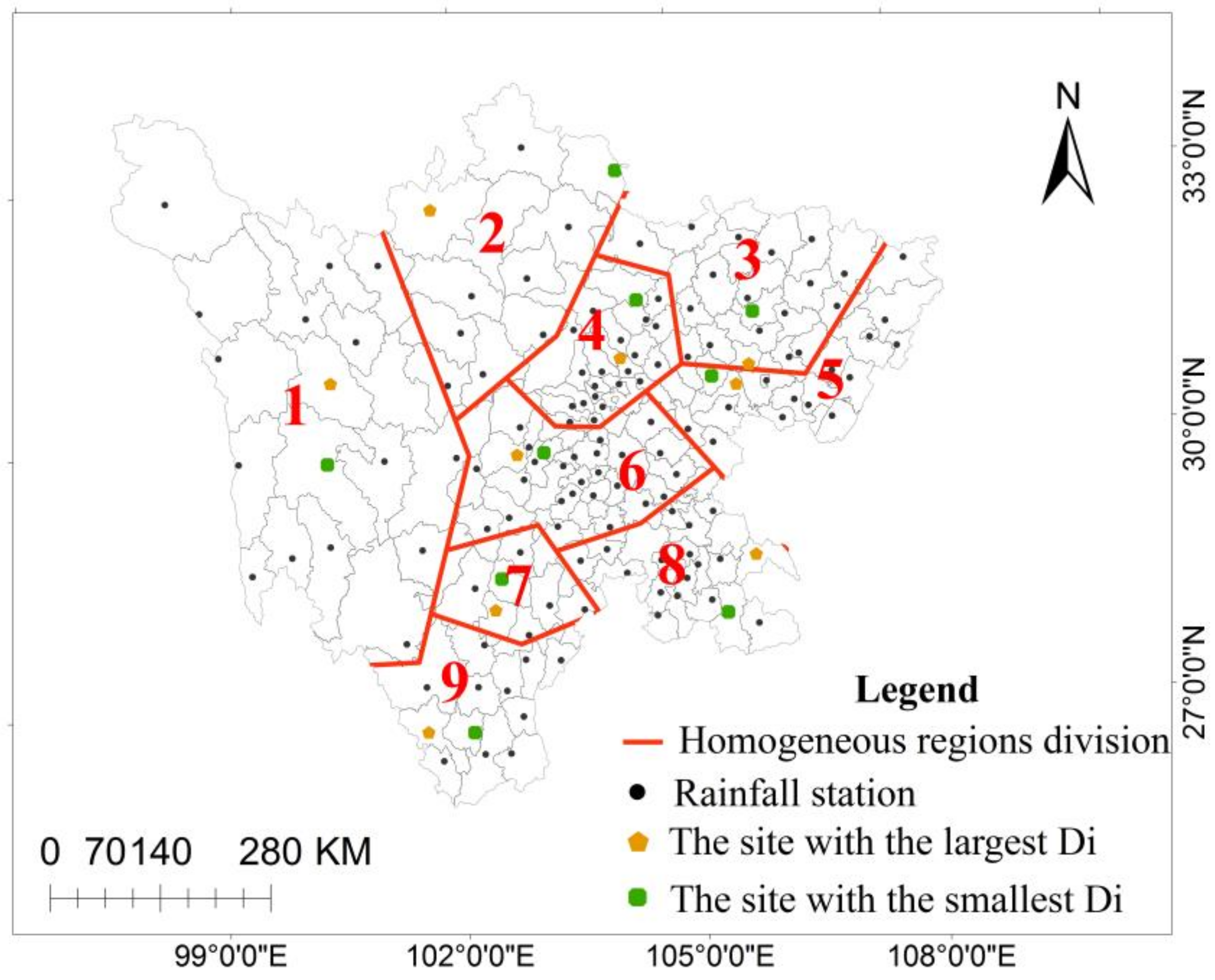
In the previous study, the annual maximum daily rainfall data series of 150 national meteorological stations in Sichuan Province were selected for hydrological frequency analysis. The maximum daily rainfall sequence length of each site was different. The longest time span was from 1951 to 2008, a total of 58 years, the shortest was 21 years, and the average observed data sequence length of each site was 51 years. Using regional frequency analysis based on L-moment, Sichuan Province was divided into nine homogeneous regions, and the optimal frequency distribution of each homogeneous region was obtained [28]. In this study, two stations were selected from each homogeneous region as the representative stations, and these two stations had the smallest and largest degrees of discordancy in the homogeneous region (Figure 1). The basic information of the selected representative sites is shown in Table 1.
2.2. Methods
2.2.1. Regional Frequency Analysis
Regional frequency analysis based on L-moments combines the L-moment method and the regional analysis method reasonably and effectively. The L-moments were originally proposed by Hosking, and was defined as a linear combination of the expected value of order statistics [29]. Compared with the ordinary moments, the error due to the second-order and third-order calculations is reduced because only the first-order moment is calculated. With better robustness and unbiasedness, it can be used to estimate parameters to achieve better results. In 1960, the regional analysis method was first proposed by Dalrymple [30], who introduced the concept of regionalization. The regional analysis method is applicable to an area with similar climatic conditions and topographical conditions, that is, the homogeneous region. This method considers that each station belonging to the same homogeneous region, that is, each station in the area with the same condition of water vapor and rainfall formation, has the same frequency distribution and parameters. The basis for hydrological frequency analysis using regional frequency analysis is to estimate the statistical parameters of rainfall data using L-moments. The definition of L-moments is as follows:
Suppose the variable X obeys a distribution function, which is the order statistic of a set of random samples, and in general, the L-moments of a probability distribution are defined by [31]:
By definition, the specific L-moments commonly used of the random variable X are:
Similar to the ordinary moments, the sample L-moment ratios are defined by:
The linear out-of-range coefficient L-Cv: ;
The linear skew coefficient L-Cs: ;
The linear kurtosis coefficient L-Ck: .
Regional frequency analysis based on L-moments was mainly divided into the following four steps: (1) data preparation works including screening the data; (2) identification of homogeneous regions; (3) choice of a frequency distribution for each homogeneous region; (4) estimation of rainfall quantiles under different return periods.
2.2.2. Data Preparation
Data for hydrological frequency analysis should be reliable, representative, and consistent [32]. Hosking et al. [31] recommended the discordancy measure to test whether the site data has singularities, thus testing the reliability and rationality of the data and improving the accuracy of the data.
Assuming that there are N stations in the region, a three-dimensional vector of the sample L-moment ratios of the annual maximum daily rainfall sequence at each site can be constructed and recorded as:
The discordant detection indicators are defined as follows:
2.2.3. Identification of Homogeneous Regions
The basic idea of using regional frequency analysis for hydrological frequency analysis is to use the homogeneous regions as the basic research unit. Therefore, the division of homogeneous regions plays an important role in the effective application of regional frequency analysis. Hosking et al. [31] proposed using the cluster analysis method, commonly used in hydrology, to preliminarily partition all stations according to the latitude, longitude, and elevation of each station and the L-moment ratios [33]. Then, the following two criteria were used to determine whether the preliminary homogeneous regions were reasonably acceptable:
- (1)
- The discordancy measure. The discordancy measure is mentioned in 2.2.2. In addition to being used to detect whether the original data is reasonable or not, the discordancy measure can also be used to test whether each site in the initially formed homogeneous region is a discordant point of the region. If the discordance statistic Di of a site exceeds the critical value, moving the site to another adjacent homogeneous region may be considered.
- (2)
- The heterogeneity measure. Hosking et al. [31] recommended the use of a heterogeneity measure to determine whether the region formed by preliminary division is a homogeneous region. The calculation formula for the heterogeneity measure is as follows:where ni is the length of the rainfall data series of the i-th station in the homogeneous region, ti is the L-Cv of the i-th station in the homogeneous region, N is the total number of stations in the homogeneous region, and μv and σv are the mean and mean square error of V1 obtained by Monte Carlo simulations, respectively. H1 < 1 indicated that the area was an acceptable homogeneous region, 1 ≤ H1 < 2 indicated that the area was a possible heterogeneous area, and H1 ≥ 2 indicated that the area was a heterogeneous area. If the value of H1 did not meet the standard, the site within the region needed to be adjusted until it met the criteria to become an acceptable homogeneous region. According to experience, there were several useful ways to adjust the sites: (1) move a site or few sites from one region to the adjacent one; (2) subdivide the region; (3) merge two or more regions and redefine groups; and (4) break up the region by reassigning its sites to other regions.
2.2.4. The Optimal Frequency Distribution
There are dozens of frequency distributions used for hydrological frequency analysis [34]. Each country has different selection criteria for the frequency distribution, which is mainly related to the natural geographical conditions and meteorological conditions of each country. Regional frequency analysis assumes the commonly used five types of three-parameter distributions are the best frequency distributions that can be fitted in each homogeneous region: generalized Pareto distribution (GPA), generalized extreme-value distribution (GEV), generalized logistic distribution (GLO), generalized normal distribution (GNO), and Pearson type III distribution (PE3). When these three-parameter frequency distributions do not fit well with the rainfall data, we can also consider fitting with a four-parameter Kappa distribution or a five-parameter Wakeby distribution. Hosking et al. [31] recommended a Monte Carlo simulation test (ZDIST) to determine the optimal frequency distribution for each homogeneous region.
Suppose that the number of stations in a homogeneous region is N, where the data length of the i-th station is ni, and the sample L-moment ratios of the station are, respectively, t(i), t3(i), t4(i), and the tR, t3R, and t4R are, respectively, the corresponding weighted average of the measured maximum annual rainfall sequence length of all stations in the homogeneous region, and t4m is the regional average linear kurtosis coefficient for the mth simulation result.
It is assumed that each site in the homogeneous region conformed to the Kappa distribution, and the Monte Carlo simulation was used to simulate. Each simulation generated data with the same length of the historical measured rainfall data sequence corresponding to each site. For the mth simulation result, the deviation of the regional average linear kurtosis coefficient t4m is as follows:
where the standard deviation of the Ck of the corresponding simulation data is as follows:
Then, the expression of the statistic ZDIST of the goodness-of-fit test is:
When the absolute value of ZDIST was not more than 1.64, the fitting result of the frequency distribution was considered to be acceptable. And the closer to 0, the better the fitting effect of the frequency distribution was, and the corresponding frequency distribution was the optimal regional frequency distribution.
2.2.5. Rainfall Estimation
Regional frequency analysis used the index flood method to estimate quantiles under different return periods of each station. The index flood method was originally proposed by Dalrymple [30]. The specific steps are as follows:
- (1)
- The annual maximum daily rainfall data of each station in the homogeneous region is averaged to generate a new rainfall data sequence. The calculation expression is as follows:where j = 1,2,……; i = 1,2,……N; Qij represents the measured rainfall data sequence of the i-th site; and is the average rainfall value of the measured rainfall data sequence of the i-th site.
- (2)
- The L-moment parameters L-Cv, L-Cs, and L-Ck, and the weighted average of the L-moment parameters of each station in each homogeneous region are obtained, that is, the regional average L-moment parameters of the homogeneous region is obtained. Its calculation expression is:where tR and trR are the weighted average of the L-moment parameters of each station in each homogeneous region. N is the number of sites in the region, ni is the measured rain data sequence length for the i-th site.
- (3)
- Estimate the distribution function parameters of the optimal frequency distribution of the region determined by the goodness-of-fit test, and then the quantiles under different return periods are obtained by the quantile functions of the chosen frequency distribution.
- (4)
- The principle of the index flood method is to treat the rainfall at each site as two components, one representing the rainfall unique to the site and the other representing the rainfall that reflects the rainfall characteristics common to the homogeneous region. The quantiles under different return periods represent the rainfall characteristics shared by the reaction area and the unique rainfall characteristics of the site, that is, the multi-year average rainfall of the site. The expression of the rainfall estimation is as follows:where QT,i,j is the estimation of the rainstorm in which the return period of the j-th station is in the i-th region. qT,i is the quantile corresponding to the return period of the i-th region. is the average annual maximum daily rainfall for site j.
2.2.6. Traditional At-Site Hydrological Frequency Analysis
Between 1880 and 1890, Hersehel et al. in the United States took the lead in applying the frequency distribution [35], and research by scholars from various countries on the analysis of hydrological frequencies also began. In 1924, Foster proposed the application of the type III distribution for hydrological frequency analysis and made the H-value table of the average coefficient, which brought convenience to frequency calculations and was widely used [36]. Domestic research on hydrological frequency analysis began in the 1930s. After the founding of New China in 1949, in order to promote the development of water conservancy, Chinese scholars began to conduct a large number of research studies on hydrological frequency analysis based on foreign experience. In November 1956, at the national academic seminar on hydrological analysis, domestic scholars discussed the sample selection method, empirical frequency formula, statistical parameter estimation, frequency distribution, sampling error, and research direction in hydrological frequency analysis. The two major problems in hydrological frequency analysis are choosing the appropriate frequency distribution and estimating the parameters of the frequency distribution. With the study of hydrological frequency analysis by scholars from all over the world, scholars from all over the world obtained good research results on how to use the hydrological data of a single station for hydrological frequency analysis. According to their own actual conditions, each country selects the most suitable empirical frequency formula, the estimation method of statistical parameters, and the frequency distribution, which is applied to the research and application of hydrological frequency analysis.
The choice of frequency distribution varies greatly from country to country. More than 20 kinds of frequency distributions are commonly used [37]. In China, on the basis of learning successful experiences in western countries, many domestic scholars conducted research on hydrological frequency analysis and achieved valid results. In 1979, the Ministry of Water Resources and the Ministry of Power Industry issued the “Water Resources and Hydropower Engineering Design Flood Calculation Specification SDJ22-79 (Trial)” [38], which unified China’s flood design standards for the first time [39]. Through the verification of China’s hydrological data, domestic scholars believe that Pearson III distribution is suitable for most of China’s hydrological situations. Therefore, currently, Pearson III distribution is generally selected for hydrological frequency analysis in China, and other frequency distributions can be selected for special cases after professional verification [40]. Commonly used parameter estimation methods include the conventional moment method, probability weight moment method, weight moment method, L-moments method, and the maximum likelihood method. Chinese hydrologists have done a lot of research on parameter estimation methods, and now the curve-fitting method is widely used. The curve fitting method is divided into the empirical fitting method and optimal fitting method. The randomness of the empirical fitting method is very strong, which is mainly determined according to the experience of the person carrying out the study. The quality of the fitting between the empirical data and the theoretical curve depends on the visual inspection of workers, so the results are often different from person to person. The optimal fitting method refers to the method for determining the parameters of the optimal frequency distribution fitted with the empirical point under the premise of certain fitting criteria. The optimal fitting method can avoid the randomness of the empirical fitting method in the process of adapting the curve. The fitting criterion is a clear criterion for judging the result of fitting. Taking the hydrological frequency analysis in China as an example, in general, the main steps of traditional at-site hydrological frequency analysis are as follows: (1) organize the hydrological sequence data of the site, analyze the reliability, consistency, and representativeness of the data so as to satisfy the premise of hydrological analysis and improve the estimation accuracy; (2) calculate the empirical frequency of historical hydrological data, and use the method of moments or other methods to estimate the initial parameters of the Pearson type III distribution for the curve fitting method; (3) draw the theoretical frequency curve based on the initial parameters, check the fitting conditions of frequency distribution and empirical data, and adjust the parameters until the fitting result is good; (4) based on the final parameters of the frequency distribution, estimate the design value of the specified return period.
3. Results
3.1. The Differences of Optimal Frequency Distributions
The selection results of frequency distributions of each representative station obtained by Monte Carlo simulation and the optimal frequency distribution of each homogeneous region obtained by previous studies are shown in Table 3. The results show that when the optimal frequency distribution was determined by Monte Carlo simulation for each representative station selected in the study, the optimal frequency distribution of each station was not necessarily the same as the optimal frequency distribution of the corresponding homogeneous region.
3.2. Comparison of Fitting Results
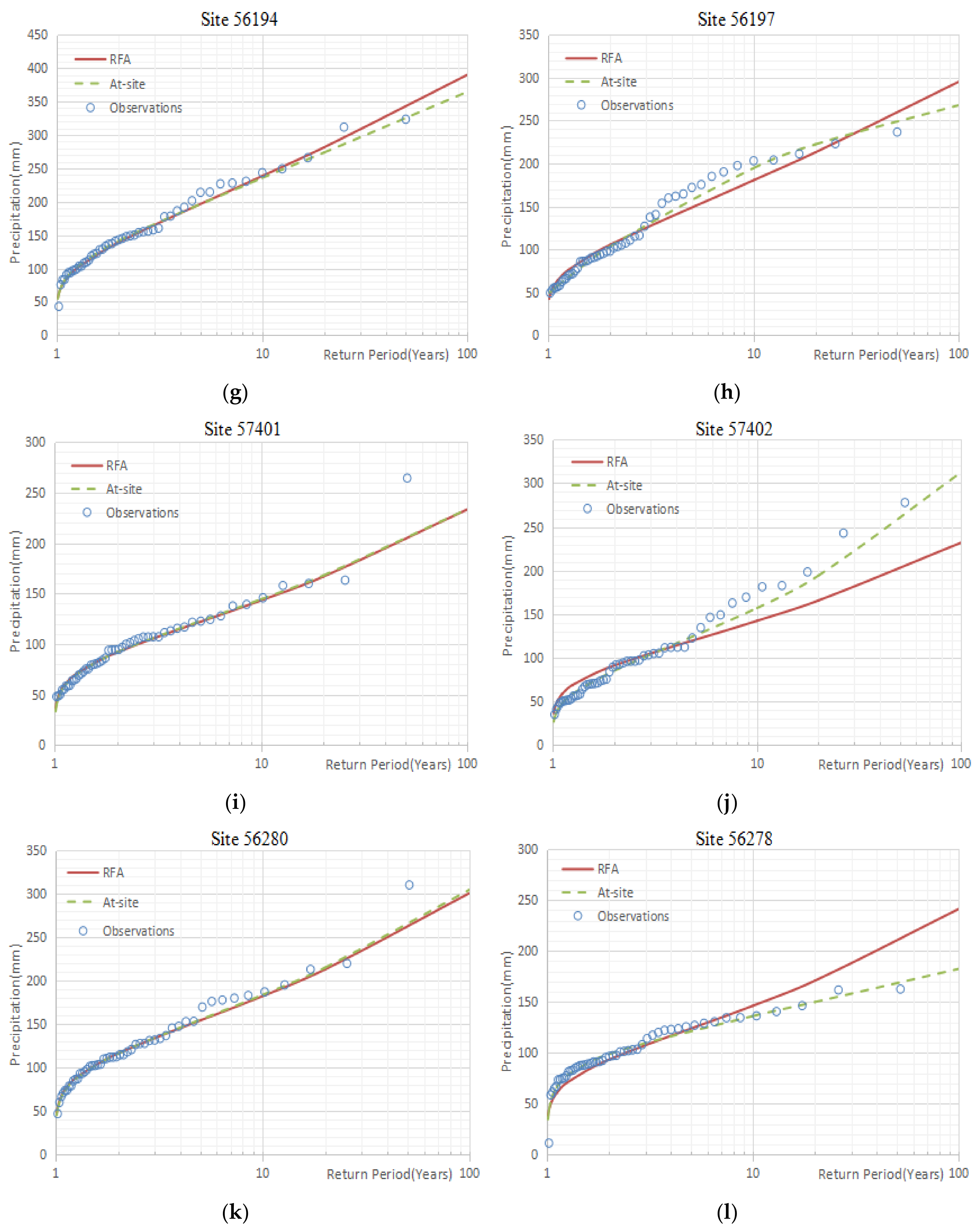
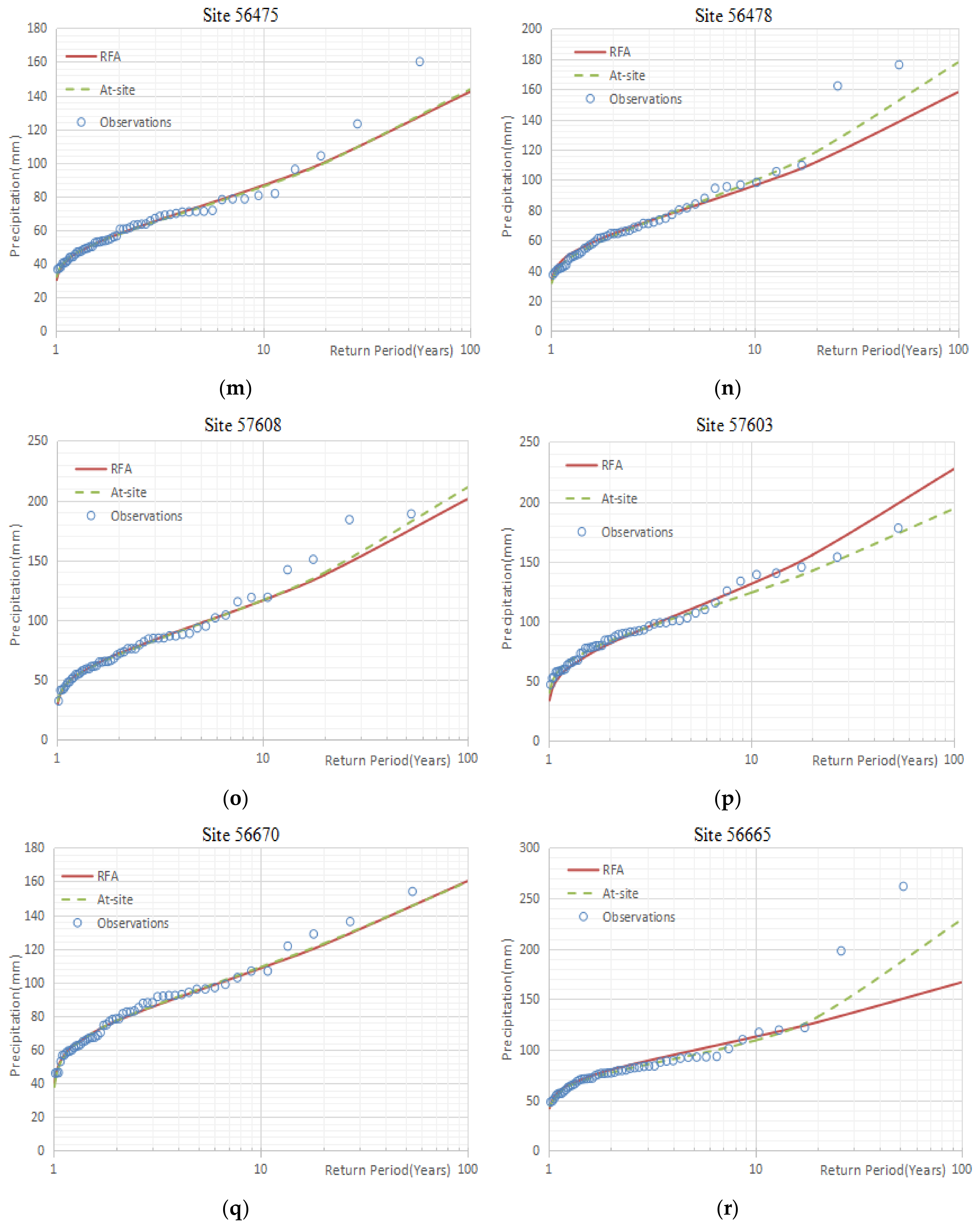
The results of hydrological frequency analysis of representative stations of each homogeneous region selected in this study by using regional frequency analysis and traditional at-site hydrological frequency analysis were obtained. The fitting results between the results obtained by the two methods and the observations are shown in Figure 2. As can be seen in Figure 2, in each homogeneous region, the design frequency curves estimated by the two methods of the stations with less discordancy were better fitted with the observed maximum daily rainfall series. However, for the sites with the largest discordancy in each homogeneous region, the results of the design frequency curves calculated by regional frequency analysis fitted to observed data were not as good as the fitting results obtained by traditional at-site hydrological frequency analysis.
3.3. The Differences between the Estimations
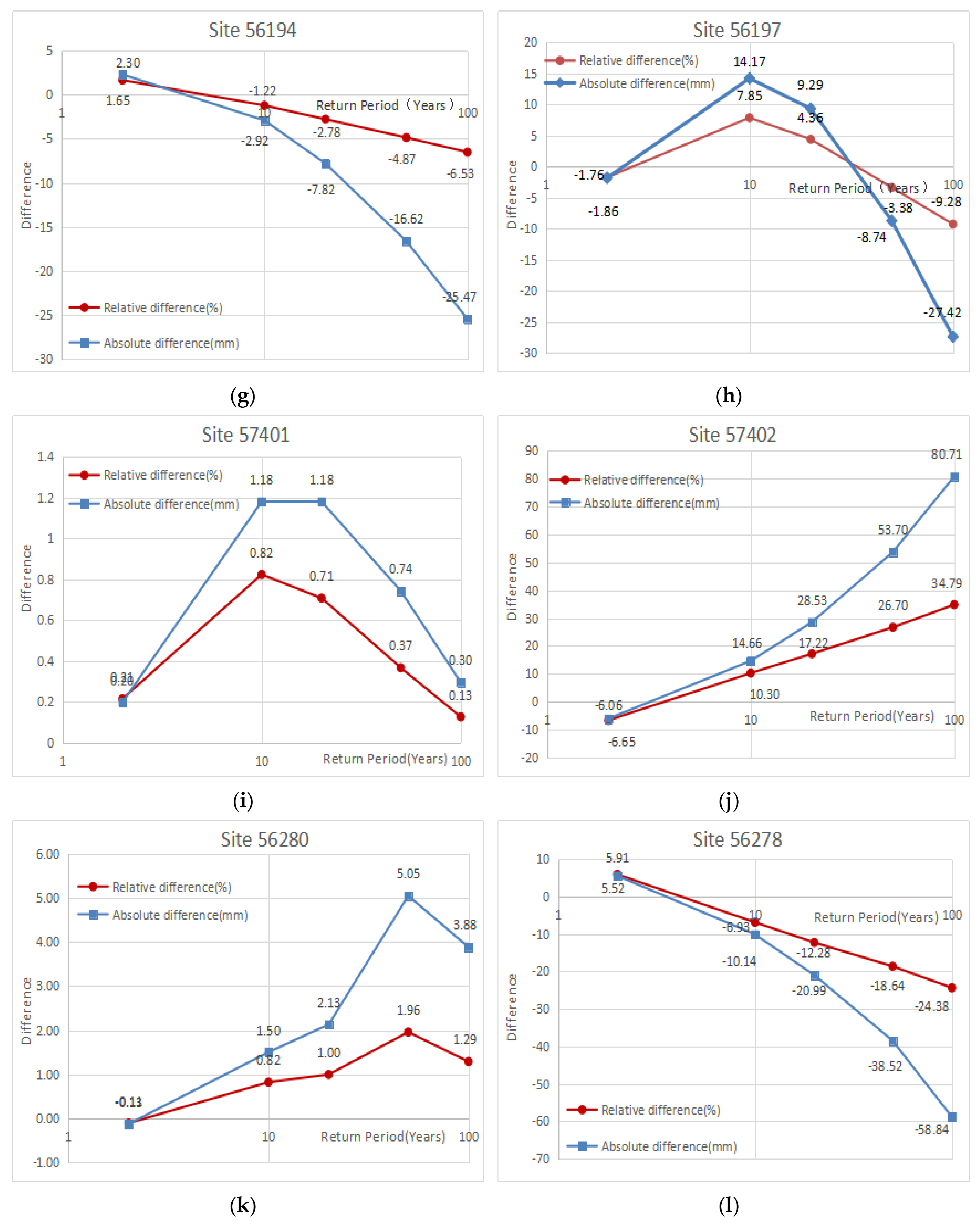
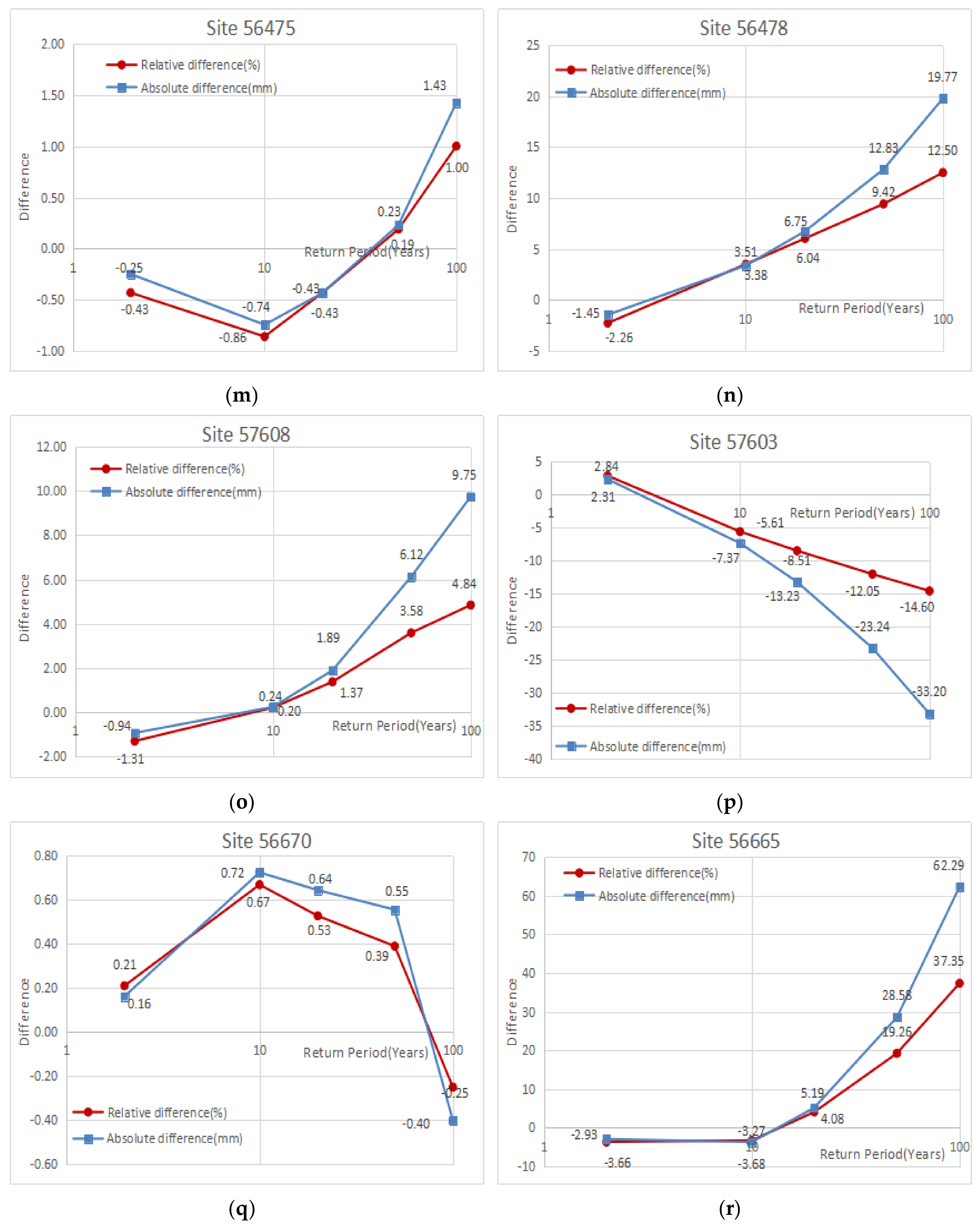
The specific differences of design values for different sites at different return periods obtained by using the two methods are shown in Figure 3. It shows that under the same return period, the difference of the design values estimated by the two methods varied from site to site; the difference between the design values obtained by the two methods using the two methods was also related to the difference in the return period. First, for the stations with the smallest discordancy in each homogeneous region, in general, the absolute differences between the design values calculated by regional frequency analysis and traditional at-site hydrological frequency analysis were very small. For the stations with the largest discordancy in each homogeneous region, the difference of the storm design values under different return periods estimated by the two methods was greater than that of the stations with the smallest discordancy under the same return period. In addition, as the return period increased, the difference between the design values obtained by regional frequency analysis and the design value estimated by traditional at-site hydrological frequency analysis also increased.
4. Discussion and Conclusions
In this paper we showed that, according to regional frequency analysis and traditional at-site hydrological frequency analysis, the optimal frequency distribution of the single station obtained by Monte Carlo simulation was not necessarily the same as the optimal frequency distribution of the corresponding homogeneous region of each station, which was related to the specific situation of the site and the homogeneous region. In addition, there was also a certain difference between the fitting results of the theoretical frequency curve obtained by the two methods with the rainfall data. And the difference between the rainfall design values obtained by traditional at-site hydrological frequency analysis and the results obtained by regional frequency analysis was different for different stations.
As shown in Table 3, the nine homogeneous regions in Sichuan Province, the optimal frequency distributions of the 1st, 2nd, 3rd, 6th, 7th, and 8th homogeneous regions were the same as the optimal frequency distributions of the representative sites in each homogeneous region, and all of them were GLO. However, the optimal frequency distributions of the regions of the 4th, 5th, and 9th regions were different from one of the representative sites in the corresponding homogeneous region. The optimal frequency distribution of the 4th homogeneous region was the GEV, and the optimal frequency distribution of the representative Site 56194 was GNO. The optimal frequency distribution of Site 56197 was GPA. The optimal frequency distribution of the 5th homogeneous region was GLO. The optimal frequency distribution of the representative Site 57401 was the same as the optimal frequency distribution of the associated homogeneous region, and the optimal frequency distribution of Site 57402 was GNO. The optimal frequency distribution in the 9th homogeneous region was GLO, and the optimal frequency distribution of Site 56670 was GLO too, but Site 56665 did not fit well with the commonly used five three-parameter distributions; therefore, the five-parameter Wakeby distribution was selected as the fitting frequency distribution of the site.
At the same time, regarding the difference in the theoretical design frequency curve of each station obtained by the two methods, in general, the difference between the design frequency curve calculated by each method was mainly reflected in the large return period, especially when the return period was greater than 10 years (Figure 2). And the difference in the design frequency curve calculated by the two methods for the stations with the largest discordancy in each homogeneous region was very apparent (Figure 2). Among them, the differences between the rainfall design values obtained by the two methods at station 56665, with a return period of 100 years in the 9th homogeneous region, had the largest deviation of 37.35 mm from the design value of rainstorm frequency obtained by using regional frequency analysis, which accounted for 62.29% of the design value obtained by using regional frequency analysis (Figure 3r). However, for the stations with the smallest discordancy in each homogeneous region, especially when the return period was 2 years, 10 years, and 20 years, the differences between the design values estimated by the two methods were almost negligible. When the return period reached 50 years and 100 years, the differences between the rainfall design values obtained by the two methods gradually increased, but overall it was still less (Figure 3). The biggest difference was the 56194 station in the 4th homogeneous region. When the return period was 100 years, the rainfall design value using traditional at-site hydrological frequency analysis method was 25.47 mm smaller than the design value obtained by regional frequency analysis, which was equivalent to 6.53% of the design value using regional frequency analysis (Figure 3g).
Furthermore, Figure 2d,f,h,j,l,n,p,r are the results of the design frequency curves obtained by the two methods fitted to observed data for the sites with the largest discordancy in each homogeneous region. The results of the design frequency curve calculated by regional frequency analysis fitted to observed data were obviously not as good as the fitting results obtained by traditional at-site hydrological frequency analysis, and there was a big difference in the design frequency curve obtained by the two methods. We believe that this was because regional frequency analysis used the homogeneous region as the research unit, and the design frequency curve of each region was obtained based on the average rainfall situation of all stations in the entire homogeneous region. The design frequency curve of each site was based on the conditions of sites. The greater the discordancy of the site, that the greater the difference between the rainfall situation of the site and the average rainfall situation relative to the homogeneous region. The results reflected the fact that regional frequency analysis considered the influence of each site on each other, which was different from traditional at-site hydrological frequency analysis.
Taking Sichuan Province as an example, we put forward a concrete representation of the specific differences between regional frequency analysis and traditional at-site hydrological frequency analysis, which can deepen the understanding of the differences between the two methods and can promote the study of hydrological frequency analysis to a certain extent. At the same time, the results of this study can also provide some reference for the flood control work in Sichuan Province.
Author Contributions
Conceptualization, M.L. and T.A.; methodology, M.L. and T.A.; software, M.L.; validation, M.L., T.A. and X.L.; formal analysis, M.L., X.L.; investigation, X.L.; resources, X.L.; data curation, M.L.; writing—original draft preparation, M.L.; writing—review and editing, T.A.; visualization, M.L.; supervision, M.L.; project administration, T.A.
Funding
This research was funded by Development of Flood Real-time Forecast System in Sichuan Province, grant number 2010HH0005.
Conflicts of Interest
The authors declare no conflict of interest.
References
- Kysely, J.; Picek, J.; Huth, R. Formation of homogeneous regions for regional frequency analysis of extreme precipitaion events in the Czech Republic. Stud. Geophys. Geod. 2006, 51, 327–344. [Google Scholar] [CrossRef]
- Okada, N.; Kusaka, T.; Sassa, K.; Takayama, T.; Sakakibara, H. Water Hazards Caused by Naturally-Occurring Hydrologic Extremes. Knowledge for Sustainable Development: An Insight into the Encyclopedia of Life Support Systems; UNESCO, EOLSS: Oxford, UK, 2002; pp. 243–263. [Google Scholar]
- Shabri, A.B.; Daud, Z.M.; Ariff, N.M. Regional analysis of annual maximum rainfall using TL-moments method. Theor. Appl. Climatol. 2011, 104, 561–570. [Google Scholar] [CrossRef]
- Ngongondo, C.S.; Xu, C.Y.; Tallaksen, L.M. Regional frequency analysis of rainfall extremes in Southern Malawi using the index rainfall and L-moments approaches. Stoch. Environ. Res. Risk Assess. 2011, 25, 939–955. [Google Scholar] [CrossRef]
- Wang, J.Q.; Gu, W.Y.; Yao, H.M. Seasonal variations of precipitation and rainstorm in China. Adv. Water Sci. 1997, 8, 108–116. [Google Scholar]
- Khan, S.A.; Hussain, I.; Hussain, T.; Faisal, M.; Muhammad, Y.S.; Shoukry, A.M. Regional frequency analysis of extremes precipitation using L-moments and partial L-moments. Adv. Meteorol. 2017, 2017, 6954902. [Google Scholar] [CrossRef]
- Hossein, M.; Arash, Z.G. Regional frequency analysis of daily rainfall extremes using L-moments approach. Atmósfera 2014, 27, 411–427. [Google Scholar]
- Zhang, Q.; Xiao, M.; Singh, V.P.; Li, J. Regionalization and spatial changing properties of droughts across the Pearl River Basin, China. J. Hydrol. 2012, 472–473, 355–366. [Google Scholar] [CrossRef]
- Abolverdi, J.; Khalili, D. Development of regional rainfall annual maxima for southwestern Iran by L-moments. Water Resour. Manag. 2010, 24, 2501–2526. [Google Scholar] [CrossRef]
- Smithers, J.C.; Schulze, R.E. A methodology for the estimation of short duration design storms in South Africa using a regional approach based on L-moments. J. Hydrol. 2001, 241, 42–52. [Google Scholar] [CrossRef]
- Lin, B.; Bonnin, G.M.; Martin, D.L. Regional Frequency Studies of Annual Extreme Precipitation in the United States Based on Regional L-Moments Analysis; ASCE Proceedings: Omaha, NE, USA, 2006. [Google Scholar]
- Haddad, K.; Rahman, A. Regional flood frequency analysis in eastern Australia: Bayesian GLS regression-based methods within fixed region and ROI framework—Quantile regression vs. parameter regression technique. J. Hydrol. 2012, 430–431, 142–161. [Google Scholar] [CrossRef]
- Durocher, M.; Burn, D.H.; Zadeh, S.M. A nationwide regional flood frequency analysis at ungauged sites using ROI/GLS with copulas and super regions. J. Hydrol. 2018, 567, 191–202. [Google Scholar] [CrossRef]
- Abdi, A.; Hassanzadeh, Y.; Talatahari, S.; Fakheri-Fard, A.; Mirabbasi, R.; Ouarda, T.B.M.J. Multivariate regional frequency analysis: Two new methods to increase the accuracy of measures. Adv. Water Resour. 2017, 107, 290–300. [Google Scholar] [CrossRef]
- Chen, Y.F.; Wang, Q.R.; Sha, Z.G. Application of L-moment based regional flood frequency analysis method to middle and lower Yangtze River. J. Hohei Univ. Nat. Sci. 2002, 31, 207–211. [Google Scholar]
- Wu, J.M.; Lin, B.Z.; Shao, Y.H. Application of regional L-moments analysis method in precipitation frequency analysis for Taihu Lake Basin. J. China Hydrol. 2015, 35, 15–22. [Google Scholar]
- Shao, Y.H.; Wu, J.M.; Li, M. Frequency analysis of extreme precipitation in Huaihe River Basin based on hydrometeorological regional L-moments method. J. China Hydrol. 2016, 36, 16–23. [Google Scholar]
- Xiong, L.H.; Guo, S.L.; Wang, C.J. Advance in regional flood frequency analysis from abroad. Adv. Water Sci. 2004, 15, 261–267. [Google Scholar]
- Li, M.; Lin, B.Z.; Shao, Y.H. Study on spatial continuity of precipitation quantile estimates based on regional L-moments analysis. J. China Hydrol. 2015, 35, 14–19. [Google Scholar]
- Liang, Y.Y.; Liu, S.G.; Zhong, G.H. Comparison between conventional moments and L-moments in rainfall frequency analysis for Taihu Lake Basin. J. China Hydrol. 2013, 33, 16–21. [Google Scholar]
- Hassan, B.G.H.; Ping, F. Regional rainfall frequency analysis for the luanhe basin—By using L-moments and cluster techniques. APCBEE Procedia 2012, 1, 126–135. [Google Scholar] [CrossRef]
- Liang, Y.; Liu, S.; Guo, Y. L-moment-based regional frequency analysis of annual extreme precipitation and its uncertainty analysis. Water Resour. Manag. 2017, 31, 3899–3919. [Google Scholar] [CrossRef]
- Yang, T.; Chen, X.; Yang, H.W.; Xie, H.W. Regional flood frequency analysisin in Pearl River Delta region based on L-moments approach. J. Hohei Univ. Nat. Sci. 2009, 37, 615–619. [Google Scholar]
- State Environmental Protection Administration. National Ecological Status Survey and Assessment; China Environmental Science Press: Beijing, China, 2006. [Google Scholar]
- Chen, C.; Pang, Y.M.; Pan, X.B.; Wang, C.Y. Analysis on change of reference crop evapotranspiration and climatic influence factors in Sichuan. Chin. J. Agrometeorol. 2011, 32, 35–40. [Google Scholar]
- Zhou, C.Y.; Cen, S.X.; Li, Y.Q. Precipitation variation and its impacts in Sichuan in the last 50 years. Acta Geogr. Sin. 2011, 66, 619–630. [Google Scholar]
- Du, H.M.; Yan, J.P. Climatic change and drought-flood regional responses in Sichuan. Resour. Sci. 2013, 35, 2491–2500. [Google Scholar]
- Li, M.R.; Ao, T.Q.; Li, X.D. Regional L-moments analysis-based study on hydrological frequency analysis of Sichuan Province. Water Resour. Hydropower Eng. 2018, 49, 54–61. [Google Scholar]
- Hosking, J.R.M. L-moments: Analysis and estimation of distributions using linear combinations of order statistics. J. R. Stat. Soc. Ser. B Methodol. 1990, 52, 105–124. [Google Scholar] [CrossRef]
- Dalrymple, T. Flood Frequency Analysis. Manual of Hydrology: Part 3. Flood-Flow Techniques. Water Supply Paper 1543-A; United States Geological Survey: Reston, VA, USA, 1960; 8p. [Google Scholar]
- Hosking, J.R.M.; Wallis, J.R. Regional Frequency Analysis: An Approach Based on L-Moments; Cambridge University Press: Cambridge, UK, 1997. [Google Scholar]
- Hemin, S.; Wang, G.J.; Li, X.C.; Chen, J.; Su, B.D.; Jiang, T. Regional frequency analysis of observed sub-daily rainfall maxima over Eastern China. Adv. Atmos. Sci. 2017, 34, 209–225. [Google Scholar]
- Burn, D.H. Cluster analysis as applied to regional flood frequency. J. Water Resour. Plan. Manag. 1989, 115, 567–582. [Google Scholar] [CrossRef]
- Jin, G.Y. General extreme value distribution and its application to hydrology. J. China Hydrol. 1998, 2, 10–16. [Google Scholar]
- Jin, G.Y. Principles and Methods of Hydrology Statistics, 2nd ed.; China Industry Press: Beijing, China, 1964; pp. 1–338. [Google Scholar]
- Department of Hydrology, Ministry of Water Resources. Chinese Hydrology Journal; China Water Resources and Hydropower Press: Beijing, China, 1997; pp. 214–216. [Google Scholar]
- Ministry of Water Resources; Ministry of Power Industry. Specification for Design Flood Calculation of Water Conservancy and Hydropower Projects: SDJ22-79 (Trial); Water Power Press: Beijing, China, 1980. [Google Scholar]
- Liang, Z.M.; Zhong, P.A.; Hua, J.P. Hydrology and Water Calculation, 2nd ed.; China Water & Power Press: Beijing, China, 2008; p. 27. [Google Scholar]
- Guo, S.L.; Liu, Z.J.; Xiong, L.H. Advances and assessment on design flood estimation methods. J. Hydraul. Eng. 2016, 47, 302–314. [Google Scholar]
- Ministry of Water Resources; Ministry of Power Industry. Specification for Design Flood Calculation of Water Conservancy and Hydropower Projects: SL44-2006; Water Power Press: Beijing, China, 2006. [Google Scholar]
Figure 1.
Schematic diagram of the study area and the selected representative meteorological site map.
Figure 1.
Schematic diagram of the study area and the selected representative meteorological site map.

Figure 2.
(a–r) are the results of the design frequency curves obtained by the two methods fitted to observed data for 18 representative stations. RFA: regional frequency analysis; At-site: traditional at-site hydrological frequency analysis; Observations: observed annual maximum daily precipitation data series.


Figure 3.
(a–r) are the results of the differences of rainfall design values under different return periods obtained by using regional frequency analysis and traditional at-site hydrological frequency analysis of 18 representative stations. (RFA: regional frequency analysis; At-site: traditional at-site hydrological frequency analysis; Absolute difference: the rainfall design value obtained by At-site minus the corresponding result obtained by RFA; Relative difference: the Absolute difference relative to the corresponding result obtained using RFA).


Table 1.
Basic information of the selected representative sites.
| Region | Name | Number | Discordancy | Length (Years) | Average (mm) | Cv | Cs | Ck |
|---|---|---|---|---|---|---|---|---|
| 1 | Litang | 56,257 | 0.16 | 57 | 35.68 | 0.1338 | 0.1562 | 0.1660 |
| Xinlong | 56,251 | 1.96 | 50 | 28.38 | 0.1167 | 0.0577 | 0.2052 | |
| 2 | Jiuzhaigou | 56,097 | 0.2 | 50 | 30.83 | 0.1440 | 0.1723 | 0.1747 |
| A’ba | 56,171 | 1.93 | 55 | 33.22 | 0.1631 | 0.3773 | 0.3467 | |
| 3 | Liangzhong | 57,306 | 0.02 | 51 | 100.65 | 0.2101 | 0.1757 | 0.1748 |
| Xichong | 57,309 | 1.75 | 49 | 92.22 | 0.2042 | 0.1660 | 0.2385 | |
| 4 | Beichuan | 56,194 | 0.19 | 49 | 153.43 | 0.2218 | 0.1998 | 0.1557 |
| Shifang | 56,197 | 2.37 | 49 | 116.17 | 0.2531 | 0.2122 | 0.0773 | |
| 5 | Shehong | 57,401 | 0.05 | 50 | 98.34 | 0.2074 | 0.1931 | 0.1840 |
| Pengxi | 57,402 | 2.86 | 52 | 97.71 | 0.2757 | 0.2967 | 0.1890 | |
| 6 | Minshan | 56,280 | 0.06 | 50 | 125.29 | 0.2081 | 0.2135 | 0.1950 |
| Tianquan | 56,278 | 2.8 | 51 | 100.42 | 0.1591 | 0.0583 | 0.1662 | |
| 7 | Yuexi | 56,475 | 0.38 | 56 | 61.97 | 0.1732 | 0.2695 | 0.2384 |
| Xide | 56,478 | 1.58 | 50 | 68.88 | 0.2017 | 0.2868 | 0.2440 | |
| 8 | Xuyong | 57,608 | 0.11 | 52 | 78.60 | 0.2175 | 0.2795 | 0.2333 |
| Hejiang | 57,603 | 2.02 | 52 | 88.77 | 0.1752 | 0.2042 | 0.1831 | |
| 9 | Miyi | 56,670 | 0.07 | 53 | 80.44 | 0.1573 | 0.1627 | 0.1650 |
| Yanbian | 56,665 | 2.65 | 51 | 83.73 | 0.1794 | 0.3564 | 0.3705 |
Table 2.
Critical values for the discordancy statistic Di.
| Number of Sites in Region | Critical Value |
|---|---|
| 5 | 1.333 |
| 6 | 1.648 |
| 7 | 1.917 |
| 8 | 2.14 |
| 9 | 2.329 |
| 10 | 2.491 |
| 11 | 2.632 |
| 12 | 2.757 |
| 13 | 2.869 |
| 14 | 2.971 |
| ≥15 | 3 |
Table 3.
Monte Carlo simulation test results for each representative site and the optimal frequency distribution for each homogeneous region.
Table 3.
Monte Carlo simulation test results for each representative site and the optimal frequency distribution for each homogeneous region.
| Region | Site | ZDIST | At-Site Optimal Frequency Distribution | Regional Optimal Frequency Distribution | ||||
|---|---|---|---|---|---|---|---|---|
| GLO | GEV | GNO | PE3 | GPD | ||||
| 1 | 56257 | −0.83 | −1.41 | −1.39 | −1.47 | −2.57 | GLO | GLO |
| 56251 | −1.38 | −2.37 | −2.2 | −2.23 | −4.25 | GLO | ||
| 2 | 56097 | 0.21 | −0.46 | −0.55 | −0.78 | −1.95 | GLO | GLO |
| 56171 | −1.36 | −1.54 | −1.83 | −2.32 | −2.14 | GLO | ||
| 3 | 57306 | 0.25 | −0.43 | −0.52 | −0.76 | −1.91 | GLO | GLO |
| 57309 | −1.59 | −2.24 | −2.3 | −2.51 | −3.65 | GLO | ||
| 4 | 56194 | 0.8 | 0.11 | −0.04 | −0.38 | −1.46 | GNO | GEV |
| 56197 | 2.99 | 2.15 | 1.92 | 1.45 | 0.21 | GPD | ||
| 5 | 57401 | 0.14 | −0.46 | −0.58 | −0.85 | −1.81 | GLO | GLO |
| 57402 | 0.67 | 0.28 | −0.02 | −0.53 | −0.77 | GNO | ||
| 6 | 56280 | 0.05 | −0.47 | −0.63 | −0.92 | −1.7 | GLO | GLO |
| 56278 | 0.02 | −0.98 | −0.81 | −0.85 | −2.88 | GLO | ||
| 7 | 56475 | −0.41 | −0.79 | −1.01 | −1.39 | −1.75 | GLO | GLO |
| 56478 | −0.35 | −0.67 | −0.89 | −1.27 | −1.51 | GLO | ||
| 8 | 57608 | −0.16 | −0.5 | −0.72 | −1.09 | −1.38 | GLO | GLO |
| 57603 | 0.23 | −0.35 | −0.49 | −0.78 | −1.68 | GLO | ||
| 9 | 56670 | 0.36 | −0.37 | −0.43 | −0.65 | −1.94 | GLO | GLO |
| 56665 | −2.08 | −2.29 | −2.56 | −3.03 | −2.93 | Wakeby | ||
© 2019 by the authors. Licensee MDPI, Basel, Switzerland. This article is an open access article distributed under the terms and conditions of the Creative Commons Attribution (CC BY) license (http://creativecommons.org/licenses/by/4.0/).
Share and Cite
MDPI and ACS Style
Li, M.; Li, X.; Ao, T. Comparative Study of Regional Frequency Analysis and Traditional At-Site Hydrological Frequency Analysis. Water 2019, 11, 486. https://doi.org/10.3390/w11030486
AMA Style
Li M, Li X, Ao T. Comparative Study of Regional Frequency Analysis and Traditional At-Site Hydrological Frequency Analysis. Water. 2019; 11(3):486. https://doi.org/10.3390/w11030486
Chicago/Turabian StyleLi, Mengrui, Xiaodong Li, and Tianqi Ao. 2019. "Comparative Study of Regional Frequency Analysis and Traditional At-Site Hydrological Frequency Analysis" Water 11, no. 3: 486. https://doi.org/10.3390/w11030486
Note that from the first issue of 2016, this journal uses article numbers instead of page numbers. See further details here.