Article

Quantification of Stream Drying Phenomena Using Grid-Based Hydrological Modeling via Long-Term Data Mining throughout South Korea including Ungauged Areas

1
Agricultural and Water Resources Engineering, Texas A&M AgriLife Research Center at El Paso, 1380 A&M Circle, El Paso, TX 79927-5020, USA
2
School of Civil and Environmental Engineering, College of Engineering, Konkuk University, 120 Neungdong-ro, Gwangjin-gu, Seoul 05029, Korea
*
Author to whom correspondence should be addressed.
Water 2019, 11(3), 477; https://doi.org/10.3390/w11030477
Submission received: 28 January 2019 / Revised: 28 February 2019 / Accepted: 3 March 2019 / Published: 7 March 2019
(This article belongs to the Special Issue Study for Ungauged Catchments—Data, Models and Uncertainties)

Abstract

:
The Drying Stream Assessment Tool and Water Flow Tracking (DrySAT-WFT) were modified to simulate the hydrological components of water loss databases (DBs) affecting stream drying phenomena. In this study, the phenomenon is defined based on a method using the 10-day minimum flow (reference Q355). Prior to identifying the method using reference Q355, the DrySAT-WFT model was calibrated and verified for its performance with the total runoff (TQ), evapotranspiration (ET), and soil moisture (SM) at 12 streamflow locations, 3 ET locations, and 58 SM locations. The average R2 for TQ in 2005 to 2015 were 0.66 to 0.84, which demonstrates good performance. Moreover, Nash Sutcliffe model efficiency (NSE) values were 0.52 to 0.72, which are also good. After verifying the DrySAT-WFT model for hydrologic components, in order to apply the method, this study defined the drying progress which was analyzed by the stream drying index (SDI) as decision criteria. In this study, the criteria for the estimation of SDI were calculated as reference Q355 coming from the 10-day minimum flow considering only weather changes from 1976 to 2015. Then, SDI grades were determined by counting the number of days below a reference Q355 from TQ considering all water loss databases (DBs) such as weather changes, groundwater uses, forest heights, soil depths, land use, and road network. On the other hand, SDI represents how many days below the reference Q355 increased when all water loss DBs were applied, in comparison to when only weather changes were applied. The DrySAT-WFT model simulated the hydrological components of the water balance based on each water loss DB, including the application of all DBs. As a result, the change ratios for TQ were measured: −4.8% for groundwater use (GWU), −1.3% for forest height (FH), −0.3% for road network (RN), −0.1% for land use (LU) and −0.1% for soil depth (SD). Overall, TQ values decreased by -8.4%. The change ratios for ET were measured: −2.0% for GWU, +10.5% for FH, +5.6% for RN, −1.8% for LU and +0.3% for SD. Overall, the ET values increased by +14.7%. In addition, based on all water loss DBs, the SDI was evaluated for all watersheds, which intensified recently (2006–2015). Under weather DB conditions, the average SDI was measured as 2.0 for all watersheds. Stream drying processes remained limited, requiring only monitoring. Given baseline conditions, stream drying intensified to grades of 3.1 (1976–1985), 3.2 (1986–1995), 3.3 (1996–2005) and 3.5 (2006–2015) by all water loss DBs.

1. Introduction

Nowadays, extreme floods and droughts caused by climate change are frequent all over the world. In particular, flooding has been widely studied as a significant phenomenon. But droughts are less known for a variety of reasons [1,2]. Many streams undergo dramatic drying processes, ranging from complete drying to the generation of reduced but permanent water flows. Streams often dry rapidly in the dry season, leaving a series of isolated pools during the summer. These isolated stream pools can dry completely or remain in the drying phase, depending on climate change, or hydrological, groundwater pumping and geological patterns [3]. Recent droughts have changed and highlighted the identification of stream drying phenomena, leading to an increase of large-capacity irrigation wells and groundwater pumping for various purposes, e.g., life, industry, and agriculture. In the United States, from tens of thousands of high-capacity wells, a lot of water withdrawals have negatively affected the regional hydrological cycles of aquifers and streams [4]. In South Korea, 84% of small streams have recently been reported to show drying [5], suggesting that such phenomena have been influenced by the increase of impervious areas due to urbanization and groundwater use (GWU).
Urbanized stream discharges occurring during drought seasons have been depleted because watershed hydrological cycles have been altered through the effect on impervious areas and excessive groundwater pumping. In addition, many large and small groundwater wells have been developed to fulfill the increased needs of water for agriculture and for living in urban and rural areas close to streams since 1980. In South Korea, water pumping levels in 2007 reached approximately 3735 million m3 year−1 [6]. Furthermore, over the past several decades, dramatic climate change processes have spurred increases in temperature, and have intensified rainfall without increases in total rainfall levels in each hydrologic year; this has greatly affected watershed hydrological processes, together with land use (LU) changes. These changes have rendered water resource management more difficult, especially with more severe droughts and stream drying processes occurring, which shortens return periods. The stable provision of water resources based on an understanding of the watershed hydrological cycle is becoming more essential and must be applied to adaptation plans for future climate change [7].
Stream drying phenomena occur when streams dry up. Not only are stream drying phenomena difficult to observe continuously, but additionally, quantitative approaches are difficult to apply due to the complex factors that cause stream drying [8]. In addition, as most stream drying phenomena occur in small rivers, it has been difficult to obtain hydrological data for small river watersheds [9]. The causes of stream drying are not clearly defined. Additionally, it is not easy to describe the dynamics. It is also difficult to spatiotemporally identify the effects of stream drying across whole areas [2]. Researchers who have studied the importance of stream drying phenomena have attempted to study e.g., increases in forest ET, excessive GWU, urbanization effects, and precipitation pattern changes; this research has, however, not been comprehensive, and the results lack spatiotemporal water volumes.
To study the long-term progression of stream drying phenomena, it is necessary to consider spatiotemporal changes occurring in the hydrological cycle affecting water loss components over a relevant period [10]. A grid-based model will be used to evaluate the stream drying progression for a specific stream within a watershed. The models are generally categorized as either lumped hydrological models, such as the SSARR (Streamflow Synthesis and Reservoir Regulation Model) and HEC-HMS (Hydrologic Modeling System); HRU (hydrological response unit)-based semidistributed models, such as the SWAT (Soil Water Assessment Tool) and SLURP (Semidistributed Land Use-based Runoff Processes); or distributed hydrological models, such as the VIC (Variable Infiltration Capacity), GRISMORM (grid-based soil moisture (SM) routing model [11,12]), and VfloTM. Of these models, distributed models maximize the efficient usage of spatial meteorological and topographical data while generating results using spatial variables and data for cell-based areas. Also, they are difficult to use in ungauged areas, as weaknesses in the point data scale can be overcame through distributed models. As a result of these issues, it may be concluded that long-term hydrological routing based on continuous spatial distribution is able to quantify stream drying phenomena the most effectively. From the distributed results, the stream drying potential measured at specific locations could be elucidated.
The spatial distribution of various data is required for stream drying tracking. Large amounts of streamflow soil moisture and groundwater level historical data were collected by setting up a number of monitoring stations. Determining the way to make the best of the potentially useful information hiding behind these historical data emerges as a new scientific issue for the study of stream drying phenomena. Han et al. [12] presented a groundwater level (GWL) prediction model based on a self-organizing map, stepwise cluster inference, and AR model. Farokhnia et al. [13] examined the utility of Sea surface temperature (SST) and Sea level pressure (SLP) global data for drought forecasting using data mining and Adaptive Neurofuzzy Inference System (ANFIS) techniques and their application to the Tehran Plain in Iran. Besides predictions, other stream drying tracking techniques have also been successfully applied in the mining the stream drying data [14,15,16].
The overall purpose in this study is to quantify stream drying phenomena across the whole of South Korea, including in ungauged areas. In order to do so, this study developed a tracking algorithm and a distributed model. The overall processes include the definition of water loss DBs that could be related to stream drying phenomena, DBs development for modeling, and distributed modeling, including calibration and evaluation. In particular, the evaluation process deals with analyses of changes in hydrological components coming from applying each water loss DB, defining reference Q355 and assessing the Stream Dying Index (SDI). This process calculates the SDI by counting the number of days below reference Q355 and identifying SDI grades regarding the severity of the phenomena (Figure 1). Finally, this study verifies the model results compared to the status report result measured by the field survey. At the end of the verification, this study proposes possible uses of the results to surpass the current method—that has the limitations of field surveys—which is the final goal in this study.

2. Materials and Methods

2.1. Causes of Stream Drying Phenomena

Stream drying has caused significant problems in large and small wells, especially in sensitive catchments, where interactions between aquifers and overland flows are pronounced. Water consumption, e.g., from pumping a well near to a stream, can dry the stream or intercept water [17]. The impacts of stream drying can be adverse, as it affects river quantity and quality, as well as aquatic ecology [18]. Stream drying issues have been studied extensively by numerous researchers [19,20,21,22,23,24].
As one of causes of stream drying phenomena, the ET contribution of individual trees and forests is reasonably well understood, and these processes were reported recently by Landsberg and Gower [25]. Studies have largely focused on delineation processes. Marked changes in ET have nevertheless been reported with forest growth [26,27,28,29]. The influence of ET is related to changes of tree and forest growth with the leaf area (LAI). Notably, LAI influences energy absorption and the interception of rainfall, and transpiration; it has also been shown to respond to tree growth [30,31,32]. In turn, considerable changes in water use occur with growth [27,33]. Köstner et al. [34] reported that maximum transpiration rates in trees are significantly related to tree or crop height, stem sapwood area, stem circumference, and so on.
The processes of urbanization transform areas of agriculture or forest into impervious surfaces. In turn, water flows are redistributed by manmade structures and drainage networks, which has a significant impact on hydrological conditions [35,36]. With ongoing urbanization, impermeable areas have expanded due to roofing and paving. Additionally, the improvement in urban storm discharge systems has intensified the concentrations of river discharges occurring during floods. In turn, declines in ordinary river discharges, spring water shortages, and the deterioration of groundwater have occurred. Furthermore, in terms of hydrological water cycles in urbanized areas, drought risks have become more severe, and the deterioration of water quality, cityscapes, and hydrophilic properties has occurred, due to the use of artificial storm drainage systems. In densely urbanized areas, the loss of water to green land and city trees will eventually lead to the deterioration of living conditions (e.g., the urban heat island phenomena) [37].
Tromp-van Meerveld et al. [38] examined the interrelations among soil depth (SD), SM and transpiration rates observed for a studied hillslope. The study reported measurements of the SM through a total soil depth interface over a short-term period. They reported that the difference in the average SD between the two sections was found to have a more significant effect on the calculated measurement of the total water quantity at different soil depths in each normal, wet, and dry dormant season (1 May 2002).

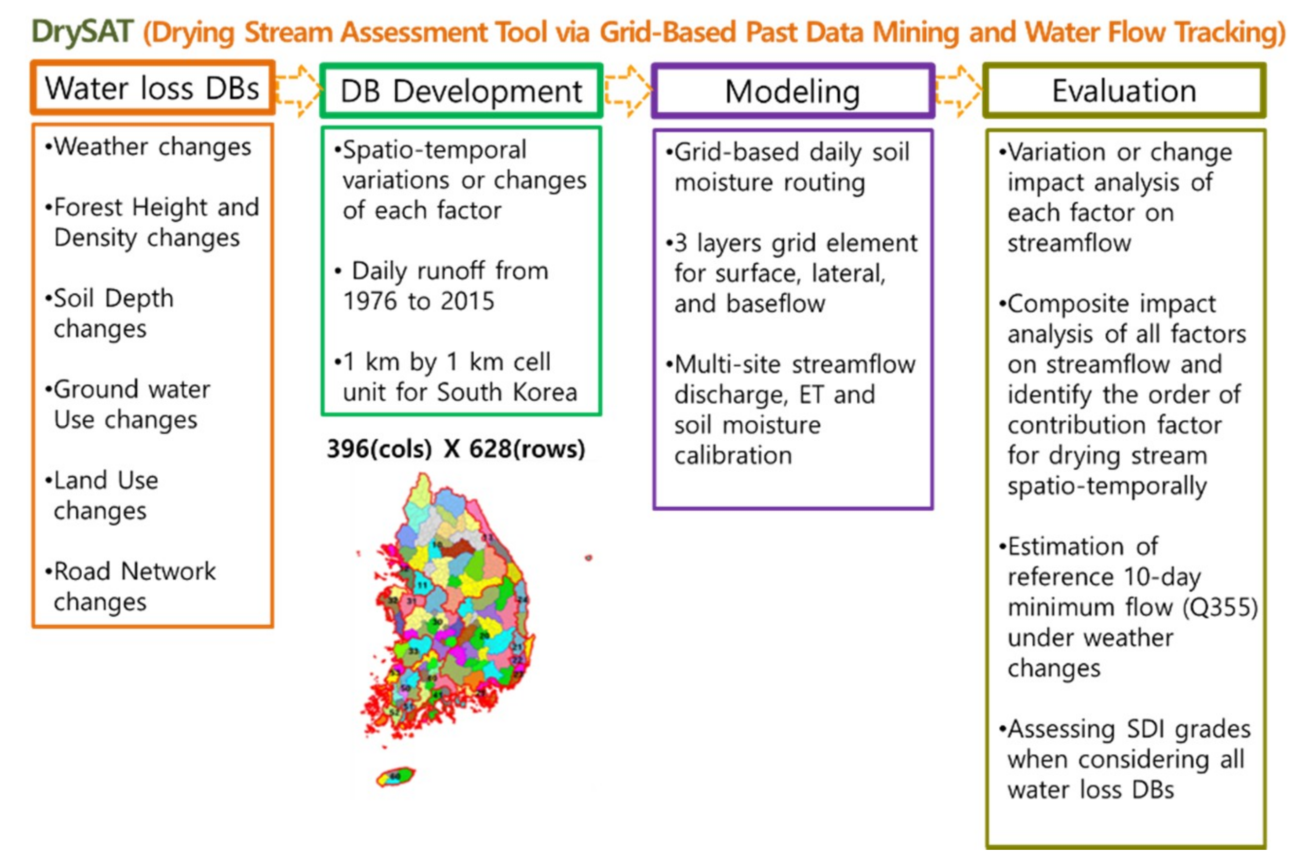
2.2. Description of Grid-Based Continuous Hydrologic Model

A physically based, continuous, long-term, distributed parameter model has been developed to assess the impacts of stream drying phenomena. The model divides the examined river basin into rectangular grid cells. A cell consists of three layers of depth. The surface runoff, lateral flow and base flow into the stream are calculated over a horizontal basis in each cell, while rainfall, ET, infiltration and percolation are calculated over a vertical basis. The daily water budget is calculated via SM routing [39] (see the Appendix A.1).
The NRCS-CN (Natural Resource Conservation Service–Curve Number) method was used to calculate the surface runoff. The surface runoff for a given day was calculated by applying the time lag of the flow and the recession curve method from the SWAT model [40] (see the Appendix A.2). This method accounts for many of the factors affecting runoff generation including soil type, land covers and land use practice, surface condition, and antecedent moisture condition (early moisture condition of the watershed prior to the storm event of interest), incorporating them in a single curve number parameter [41,42,43]. So, this study adopted this method to consider a variety of conditions such as weather, soil, and land use changes. To trace the lateral flow, the subsurface flow was calculated when the SM exceeded the field capacity [44,45] (see the Appendix A.3).
The Food and Agriculture Organization (FAO) Penman-Monteith equation was used to estimate the amount of daily ET [43] (see the Appendix A.4). There are approximately 50 methods or models available to estimate PET, but these methods or models give inconsistent values due to their different assumptions and input data requirements, or because they were often developed for specific climatic regions [46]. The Penman-Monteith method is considered the most physical and reliable method, and it is often used as a standard to verify other empirical methods. Also, this study should consider weather changes over a period of about 40 years with a variety of weather components. Thus, this ET method should be adopted to catch effects due to changes on a variety of weather components.
The leaf area index (LAI) data extracted from the satellite images were used to denote actual ET in the dynamic resistance equation [40] (see the Appendix A.5). The potential transpiration is determined from measuring atmospheric demand using pan evaporation or the Penman method [39]. The predefined crop coefficient curve does not account for the effect of water deficits, since these coefficients were established under well-watered conditions [47,48]. Plants reduce their leaf area indexes and hence, their consumption of water, under limited water conditions. The LAI is thus a potential indicator of crop water consumption [49]. So, LAI should be considered for more potential ET.

2.3. Stream Drying Phenomena Definition

Stream drying phenomena, which are often defined as long-term declines in water levels caused by sustained factors, are key issues associated with GWU, and define the reduction in stream flow rates caused by various factors which are hydraulically related to a given stream. Many areas of South Korea are undergoing stream drying phenomena. In South Korea, these phenomena have not yet been clearly defined. Generally, stream drying has been defined as when a river is almost empty enough to expose its riverbed. Thus, no criteria for defining stream drying from river flows have been developed until now. In this study, the 10-day minimum flow was defined based on the standard criteria given by the Ministry of Land, Infrastructure, and Transport [50,51]. When applying this hydrological definition, actual streamflow data must be measured from small rivers. However, because the flow rate of the studied rivers has not been measured, it is difficult to understand the stream drying processes of the present system. To overcome this problem, it was necessary to apply a grid-based distributed hydrologic model to predict the flow of a small river. In this study, the 10-day minimum flow (Q355) under only a weather DB as the baseline condition, as given by the Ministry of Land, Infrastructure, and Transport [50], was used as the reference Q355. The reference Q355 was used to quantitatively analyze the severity of the stream drying phenomena, which develops a need for creating an index, called the Stream Drying Index (SDI), for the process of a drying stream. The SDI grades were determined by counting the number of days with a minimum flow less than 10 days (reference Q355) from the runoff results when applying other water loss databases (DBs) as the artificial conditions. The SDI is evaluated on an annual basis, as shown in Table 1 [50]. All water loss DBs used in this study are detailed in Appendix B.

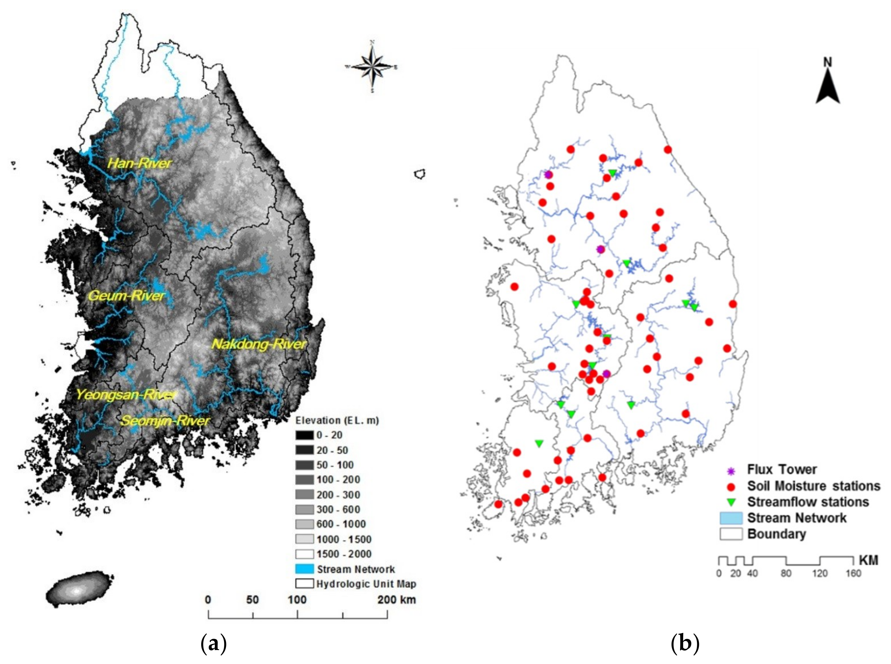
2.4. Description of the Study Area

The study area covers the total land area of South Korea, which located in northeastern Asia, within latitude and longitude ranges of 33°06′ to 43°01′ N and 124°04′ to 131°05′ E (Figure 2a), respectively. The country covers an area of 99,900 km2, and its climate is characterized by four seasons, with heavy precipitation (PCP) occurring during the monsoon summer season (June to August). Under the influence of migratory anticyclones, the spring (March to May) and fall (September to November) seasons are characterized by particularly dry weather. Winter (December to February) is characterized by a frigid climate in comparison to the other climates observed at the same latitude due to the influence of the Siberian air mass [52]. Mean annual temperatures (1981–2010) range from 6.6 °C to 16.6 °C. The mean annual PCP in South Korea ranges from 825.6 to 2007.3 mm.
As mentioned, the study area is the whole of South Korea. Thus, this study should check the ability to be able to cover spatial boundaries through the proposed algorithm and developed model.
For model calibration, the streamflow measured at 12 stations was used. Eddy covariance ET values measured at 3 flux towers (i.e., Seolmacheon (SMK), Cheongmicheon (CFK), and Deokyusan (DMK)) were used. To develop a model on the expected SM, we used the observed SM data from various stations. We used SM data measured by the Korea Meteorological Administration (KMA) at 9 stations, the Hydrological Survey Center (HSC) at 2 stations, K-water (Korea Water Resources Corporation) at 7 stations and the Korea Rural Development Administration (KRDA) at 40 stations (Figure 2b).

3. Results and Discussion

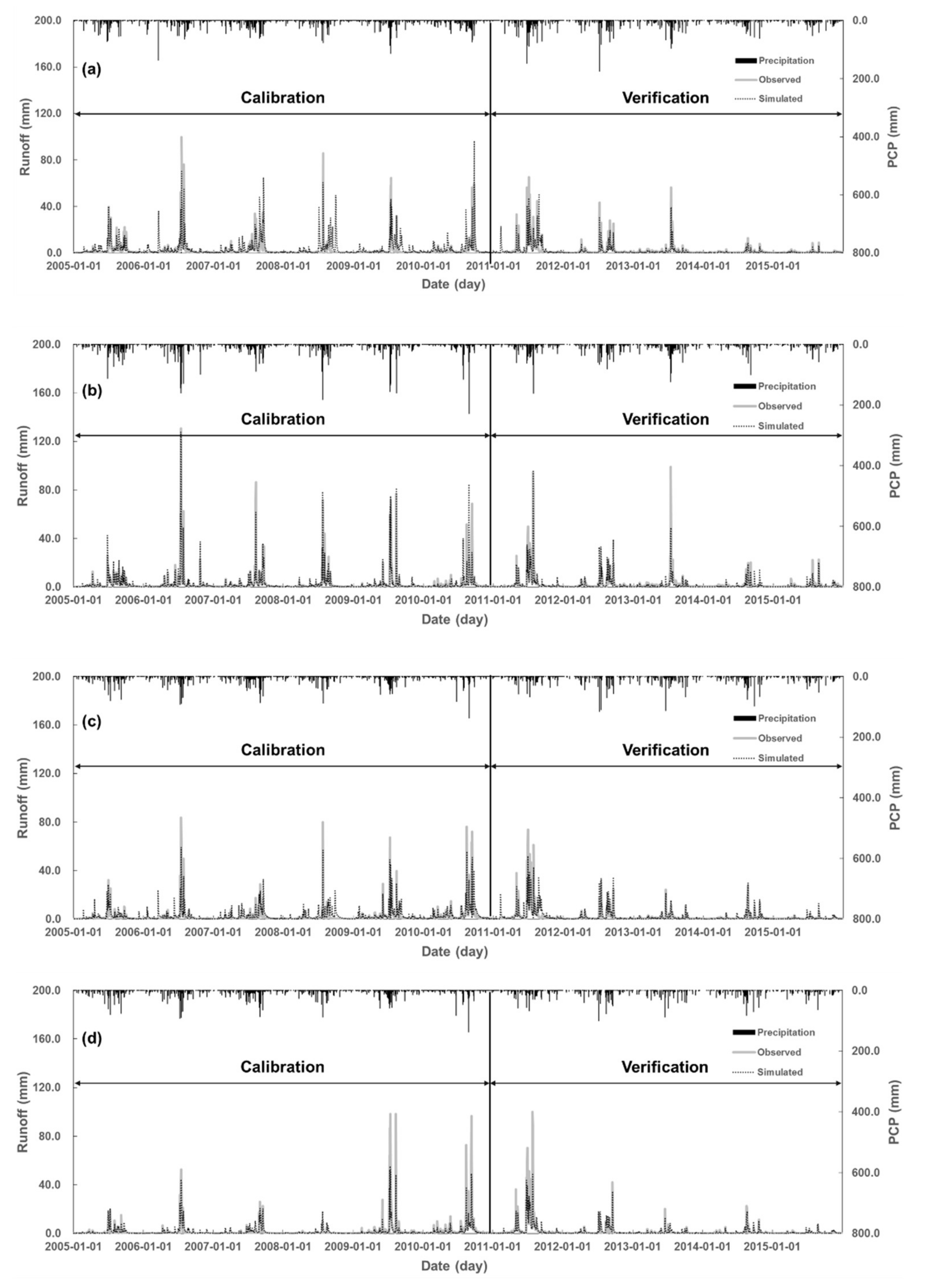
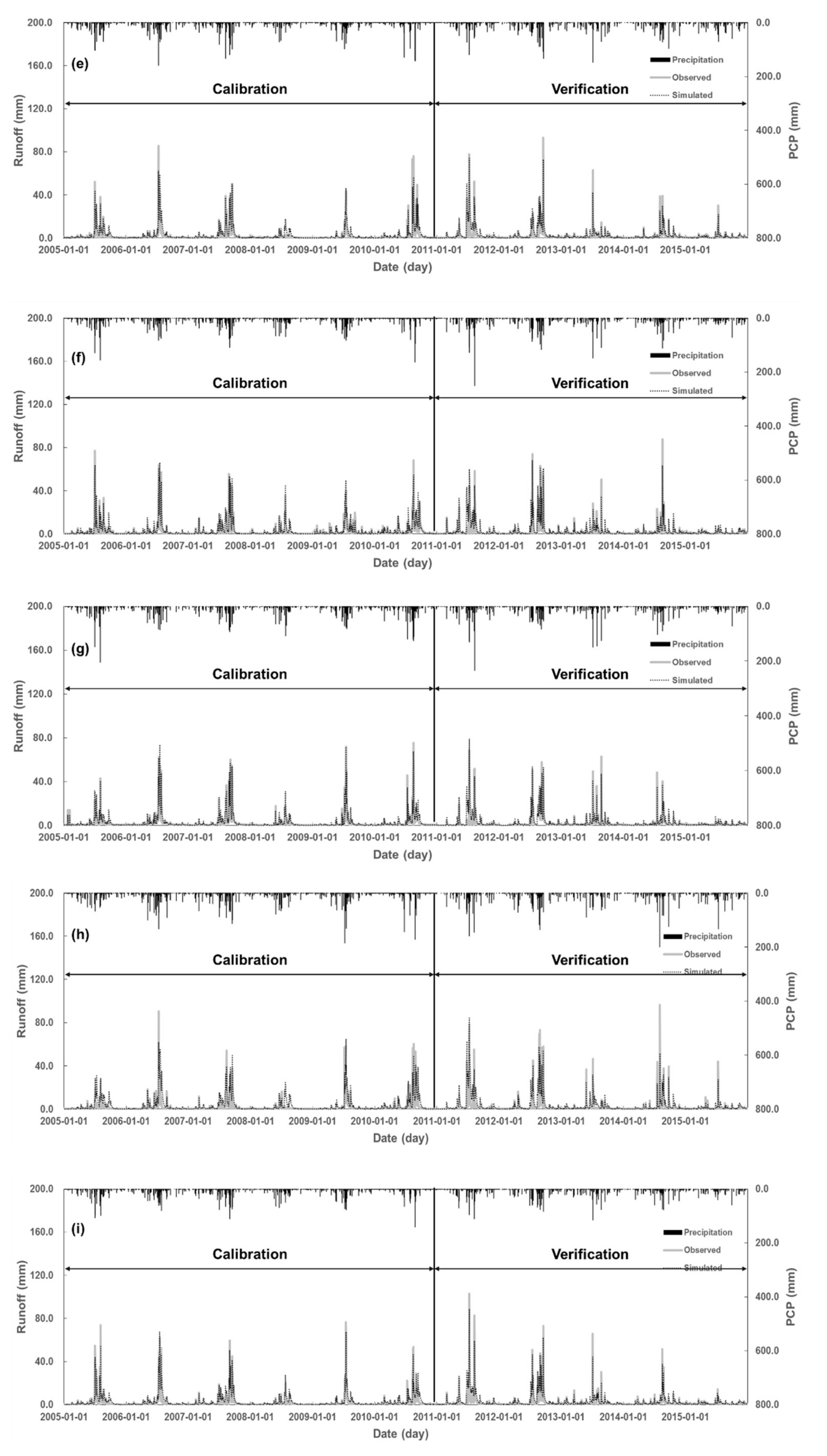
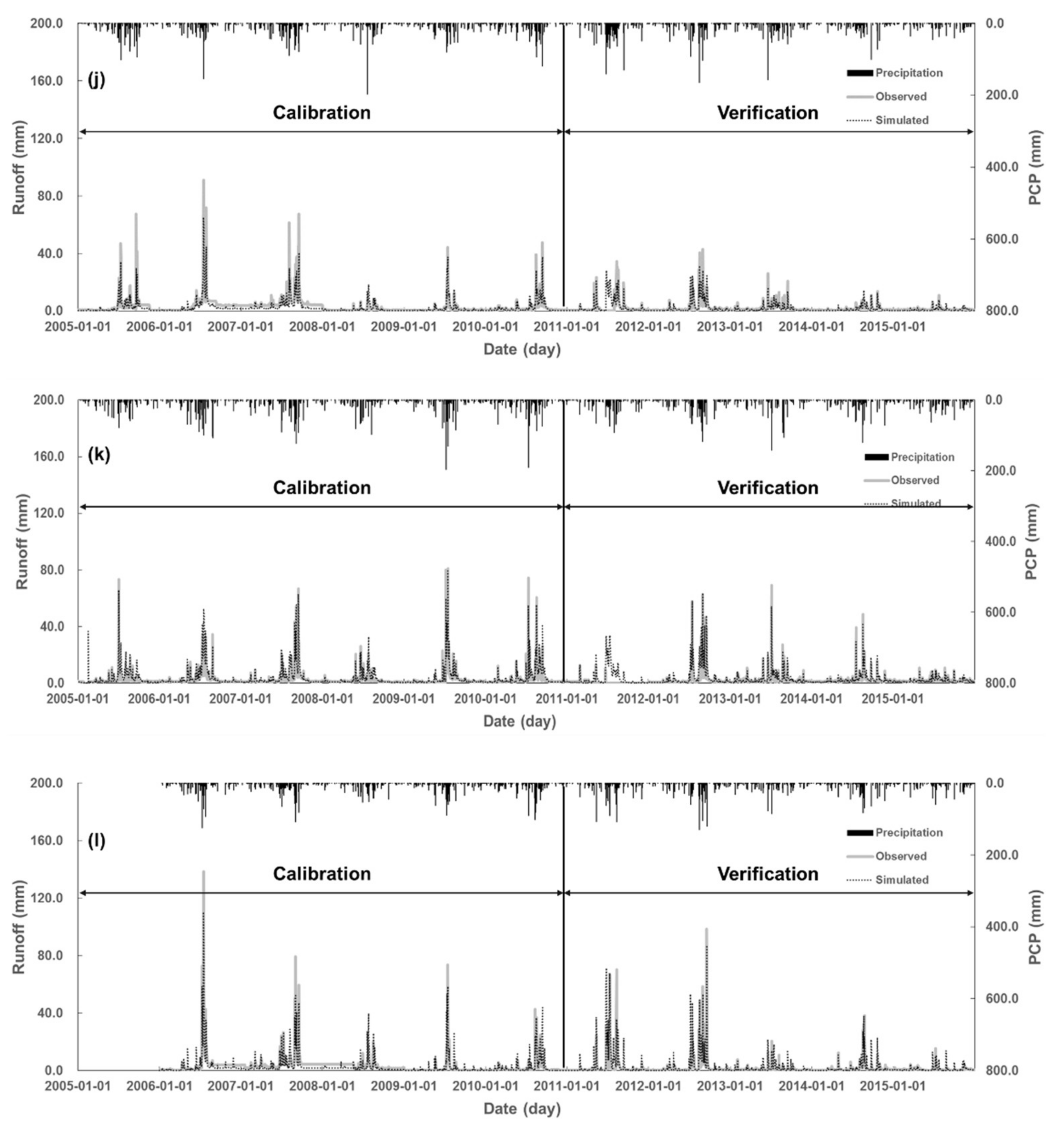
3.1. Calibration and Validation of the Model

The model was calibrated at 12 watershed outlets using 6 years (2005–2010) of streamflow data, and verified using 5 years (2011–2015) of data with averaged calibration parameters. Table 2 summarizes the parameter values determined in the 12 study watersheds. In this study, eight multipurpose dams (i.e., the Chungju dam (CJ), Soyanggang dam (SY), Andong dam (AD), Imha dam (IH), Hapcheon dam (HC), Seomjingang dam (SJ), Juam dam (JA), and Yongdam dam (YD)) and four gauging stations (i.e., Osucheon (OSC), Mihocheon (MHC), Mareuk (MR), and Chogang (CG)) were selected as the model calibration points. Surlag, which is sa urface runoff-related parameter, was highly sensitive to both the peak flow and the amount of discharge. The percolation-related parameter from the soil layer to the shallow aquifer, per_rt, was sensitive to the baseflow generation. The lateral and base flow recession control parameters slp_l and slp_b affected the recession phase of the hydrograph.
The coefficient of determination (R2) and the Nash and Sutcliffe [53] model efficiency (NSE) were used to quantitatively assess the ability of the model to replicate temporal trends in the observed hydrological data. The R2 values were defined as the square of the coefficient of correlation. The NSE ranged from −∞ to 1. A value of 1 (NSE = 1) corresponded to a perfect match between the modeled discharge and the observed data. A value of 0 (NSE = 0) indicated that the model predictions were as accurate as the mean of the observed data, whereas an efficiency of less than zero (NSE < 0) occurred when the observed mean was a better predictor than the model or residual variance (described by the numerator in the expression above) being larger than the data variance (described by the denominator) [54]. Moriasi et al. [54] recommend that three quantitative statistics—Nash-Sutcliffe efficiency (NSE), percent bias (PBIAS), and ratio of the root mean square error to the standard deviation of measured data (RSR), in addition to the graphical techniques—be used in model evaluation. In hydrologic modelling, the Coefficient of Determination is commonly known as the Nash–Sutcliffe efficiency [55].
In the case of runoff, the average model efficiency, expressed as the R2 value, was greater than 0.59. The average R2 values for the calibration (2005–2010) and validation (2011–2015) periods were 0.68 at CJ, 0.84 at SY, 0.71 at AD, 0.84 at IH, 0.82 at HC, 0.78 at SJ, 0.80 at OSC, 0.66 at JA, 0.83 at YD, 0.74 at MHC, 0.76 at MR, and 0.69 at CG. Moreover, the NSE values were 0.52 at CJ, 0.66 at SY, 0.56 at AD, 0.68 at IH, 0.67 at HC, 0.55 at SJ, 0.70 at OSC, 0.55 at JA, 0.72 at YD, 0.68 at MHC, 0.60 at MR, and 0.54 at CG, as shown in Figure 3. The average NSE of the streamflow was typically greater than 0.50, which indicated a satisfactory simulation according to Moriasi et al. [54].
For ET calibration, the model was calibrated and verified at 3 flux towers using 3 years (2013–2015) of ET data. It shows the daily time series and scatter plots for the simulated ET and flux tower ET over 5 years at 3 locations. The average NSE values of ET were 0.27 in SMK, 0.64 in CFK, and 0.37 in DMK. The ET was adjusted by controlling the CANMX parameter in Table 2. The value difference was caused by the simulation values of the recession phase in the SWAT ET being lower than the observed ET values. The average R2 values of ET were 0.43, 0.68, and 0.51, respectively. The source of the errors may be the uncertainty in the soil water consumption by plants and the lumped treatment of the soil parameters by similar units of hydrologic response in the watershed. For SM calibration, we used the measured SM values at 58 stations. The SM was calibrated using two parameters, inf_rt and per_rt, and the accuracy with respect to the observed SM was verified by the R2 values. The R2 values ranged from 0.20 to 0.68 for all stations, and the average was 0.51. The main errors of low accuracy may have been associated with the artificial water supply. Unlike other stations, these SM stations are located near upland crop and paddy field areas. Therefore, the observed SM was likely influenced by the agricultural water supply in addition to PCP during the irrigation period from April to June.

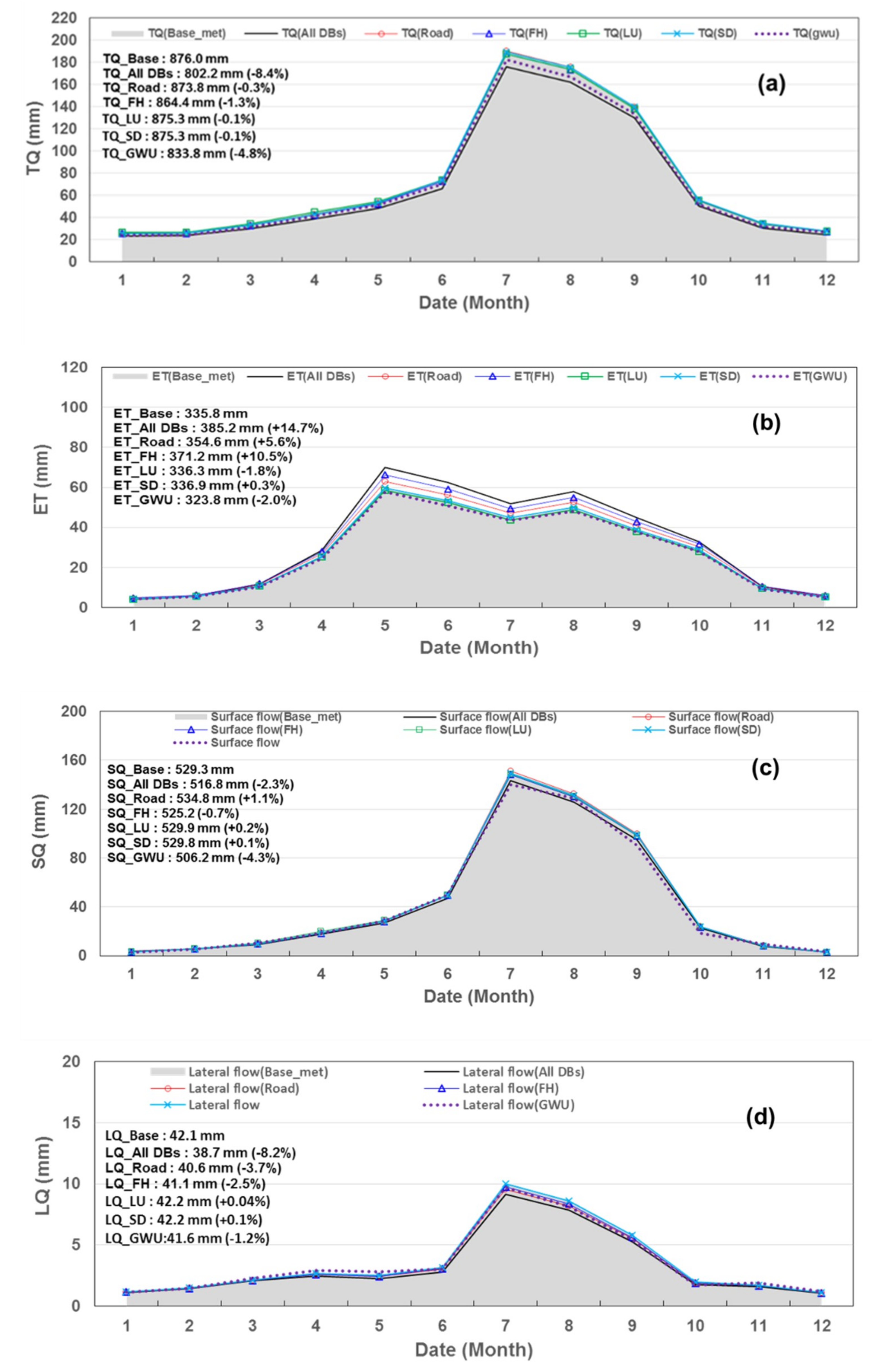
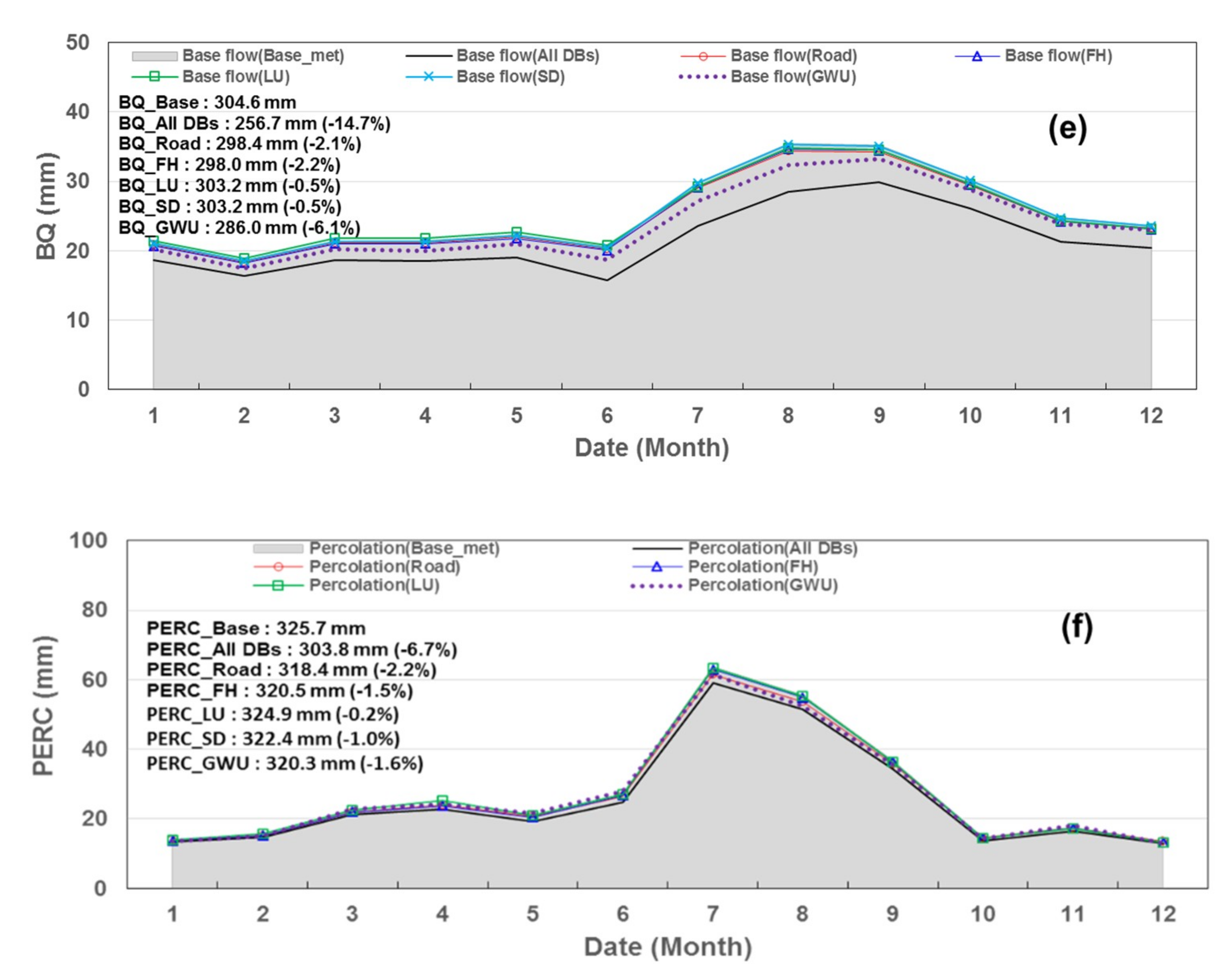
3.2. Water Balance Analysis

Using the spatially calibrated and validated DrySAT-WFT model results, a water balance analysis was conducted for a forty-year (1976–2015) to quantify the linkages between the hydrology and total water loss DBs in the study area. The vertical water budget, including ET at the surface, percolation (PERC or PC) and SM, were analyzed at the average basin scale. The horizontal water transfer was evaluated using total runoff (TQ), surface runoff (SQ), lateral flow (LQ, which originates below the surface but above the saturated zone and contributes to streamflow), and baseflow (BQ). The average annual ratios of the total runoff to precipitation over the simulation period were found to be 56.8%, 63.0%, 62.9%, and 61.8% for 1976–1985, 1986–1995, 1996–2005, and 2006–2015, respectively. Despite the gradual growth in PCP, the runoff ratio showed a gradual decline. These results showed increases in PC and SM by reducing the soil depth, a decrease in LQ by increasing the road network, a decrease in BQ by increasing groundwater use, and an increase in ET by increasing the forest height.
A monthly water balance analysis was conducted over a forty-year period (1976–2015). The simulated SQ, LQ, and BQ proportions of the study area to the total discharge were 63.2%, 4.8%, and 32.0%, respectively. The simulated SQ, LQ, and BQ values had significant seasonal periodicity, and were characterized by higher discharges (discharges of 65.8–176.0 mm) from June to September and a low-flow season (discharges of 23.3–50.4 mm) from October to May (Figure 4). These results show that the total BQ proportion to the total flow (TQ) in the low-flow season had a higher proportion (59.7%) than that (19.5%) in the high-flow season. Unlike the SQ process, BQ lagged as much as the delay time. Therefore, if BQ flows into rivers for a long time in low-flow seasons, this finding might affect stream drying phenomena.

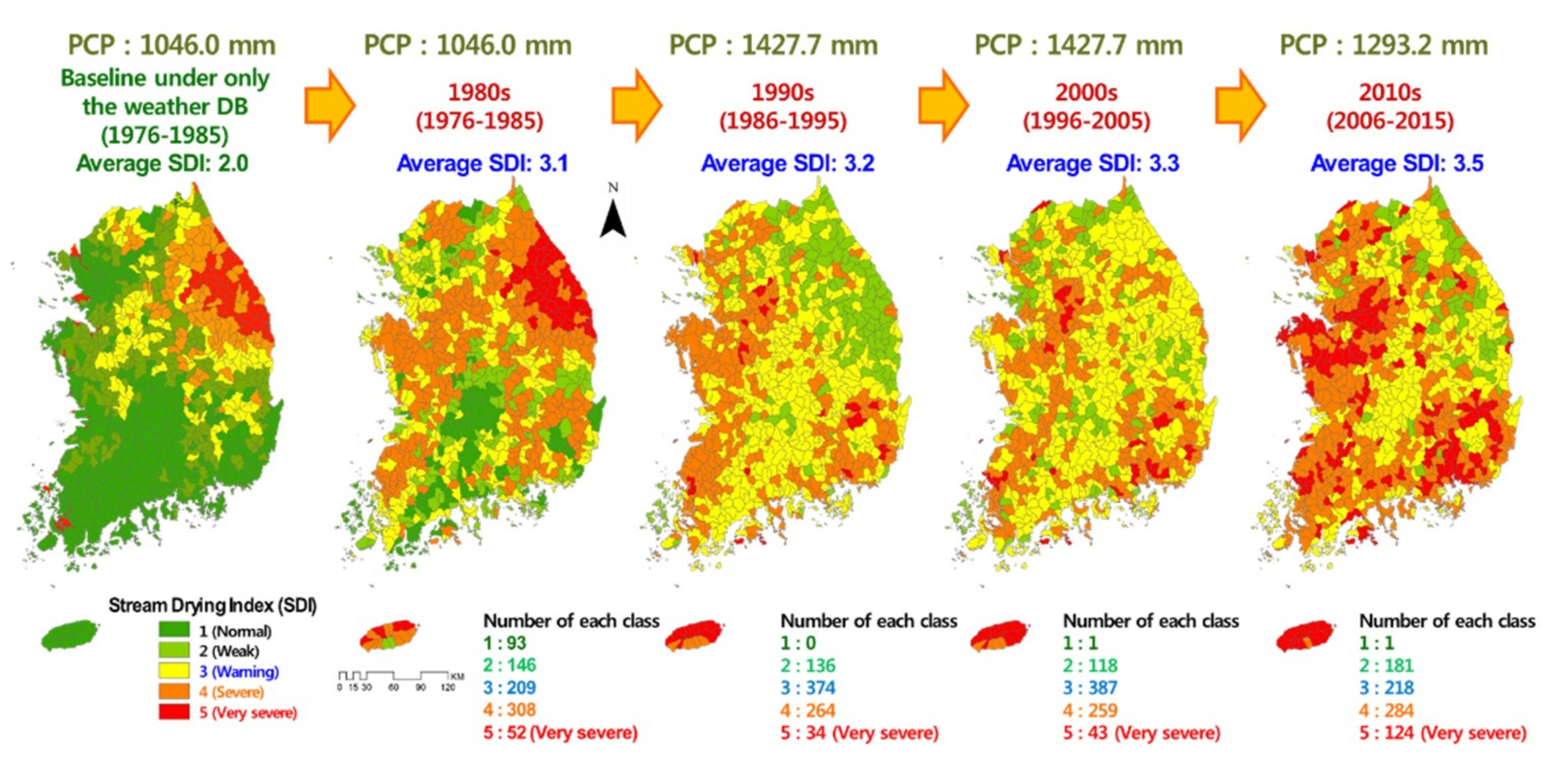
3.3. Comparison of the Stream Drying Index (SDI) Results

Prior to assessment of SDI, the 10-day minimum flow (reference Q355) over 40 years (1976 to 2015) was evaluated as the standard flow criteria suggested by the MLIT [50] when only considering weather changes except for other each water loss DB (see the Appendix B). In other words, the standard flow represented the 10-day minimum flow (reference Q355) under natural runoff conditions. The average reference Q355 values from the 1980s (1976–1985), 1990s (1986–1995), 2000s (1996–2005), and 2010s (2006–2015) were 0.37, 0.53, 0.48, and 0.44 mm, respectively. Next, as summarized in Figure 5, by applying all water loss DBs from 1976 to 2015, the modeling results for the stream drying phenomena were determined. The SDI calculated the number of days below the reference Q355 using only the weather DB in a year. The counted days were determined by finding the matching days with the SDI classes from Table 1. The SDI increased in the recent period (2006–2015). Under the weather DB conditions, the average SDI was 2.0 for all watersheds. The drying stream maintained a weak status and required only monitoring. From the baseline, the SDI increased to 3.1 (1976–1985), 3.2 (1986–1995), 3.3 (1996–2005) and 3.5 (2006–2015) in all water loss DBs.

3.4. Verification for Severity Assessment of the Model Results

Essentially, this study was intended to extend a variety of ungauged areas based on verification in a previous study [51]. The previous study was a test-bed for small watersheds to identify the algorithm when applied to steam drying phenomena. The algorithm was verified by observing data directly for the small watersheds in the previous study. In order to extend the verifications, this study used the status survey report on stream drying phenomena [6]. The report was the result of a field survey from 2001 to 2010. Thus, it could not cover the whole of Korea; only the results for the major watersheds were presented as a middle watershed size ranged from about 90 to 2500 km2. Although the watershed size ranged about 7 to 500 km2, the model results in this study are a little different from watershed size of the status report. This study compared the accuracy of the two results, i.e., the model and the status survey report, by finding matching watersheds (Table 3). Table 3 summarizes the accuracy of the two sets of results. The accuracy (%) was determined by the number of points classified correctly in total sample data from the confusion matrix. As clearly seen in Table 3, the model accuracy ranged 30.4 to 71.0%. Notably, the poor accuracy in the Han and Youngsan rivers could come from the insufficient accuracy of the water uses. The Han-river is the most densely populated area in South Korea, and it uses the most living water, with a yearly average of 2,601,875 thousand. Also, Youngsan-river is the area with the most agricultural activity; as such, it uses the most agricultural water, with a yearly average 165,919 thousand tons. In basins where living and agricultural water consumption is large, it was concluded that there is a large error in actual survey report of the stream drying phenomena and modeling results due to water usage not being recorded accurately.

4. Conclusions

This study tried to assess the impact on stream drying phenomena through a grid-based continuous model with spatial water loss DBs. The methods presented here included the DrySAT-WFT model, which was based on a new tracing algorithm for applying each water loss DBs. The following points are summarized as follows:
(1)
The stream drying phenomena were defined with the method using the 10-day minimum flow (reference Q355) by applying only the weather DB. Additionally, the DBs that can affect the stream drying phenomena were defined as water loss DBs. Then, the water loss DBs were spatially distributed from 1976 to 2015.
(2)
The modified DrySAT-WFT model was calibrated and verified with the TQ, ET, and SM. To quantify these phenomena, this study used the average reference Q355 values over 40 years. The progress of the phenomena was able to be analyzed by the SDI. The SDI grades were determined by counting days less than the reference Q355 value. The reference Q355 values from the 1980s (1976–1985), 1990s (1986–1995), 2000s (1996–2005), and 2010s (2006–2015) were 0.37, 0.53, 0.48, and 0.44 mm, respectively. Since the 1990s, the Q355 value has decreased by 16.9%. The lowest Q355 value was observed in the 1980s, which was affected by extreme droughts from 1976 to 1982.
(3)
The DrySAT-WFT model simulated the hydrological components of the water balance by each water loss DB, including the application of all DBs. As a result, the change ratios of TQ were −4.8% for GWU, −1.3% for FH, −0.3% for RN, −0.1% for LU and −0.1% for SD. Overall, the TQ decreased by −8.4%. The change ratios of ET were −2.0% for GWU, +10.5% for FH, +5.6% for RN, −1.8% for LU and +0.3% for SD. Overall, ET increased by +14.7%.
(4)
By applying all DBs, the SDI was evaluated in all watersheds. The SDI increased in the recent period (2006–2015). Under the changing weather DB conditions, the average SDI was 2.0 in all watersheds. The drying stream maintained a weak SDI grade. From the baseline, the stream drying progress increased to grades of 3.1 (1976–1985), 3.2 (1986–1995), 3.3 (1996–2005) and 3.5 (2006–2015) in all water loss DBs.
Until now, many studies of stream drying phenomena only carried out current state evaluations, and stream drying was identified by government surveys. These surveys were not only impossible to investigate in wide areas, including ungauged areas, but also could not identify the causes of the stream drying phenomena in each watershed. When it comes to the overall purpose, once again, this study was intended to quantify stream drying phenomena in whole of South Korea, including in ungauged areas. Finally, this study tried to find the dried stream regions presented by SDI using the DrySAT-WFT model and the application of data mining. This would be the final finding of this study. It can determine the severity of the stream drying phenomena as an objective indicator, and distinguish it from the drought phenomena. Therefore, it is very important thing, because it would be possible establish suitable measures and plans for the future if vulnerability due to droughts or dried streams could be determined.
The finding of this study can be clearly distinguished from those of other similar studies. Similar studies have been conducted to identify drought phenomena. Droughts are an indicator that would suggest dried streams, but this is not clear for stream drying phenomena. In addition, it is difficult to use droughts as integrated indicators because there are many indicators that can judge several droughts. Most of all, the significant difference is that stream drying phenomena are caused by an accumulation of the influences of various factors over a long period of time, while droughts are occur at a specific time for short periods.
The results of this study are very useful in practical applications and can be used as basic information index to determine river maintenance flows for decision makers, especially in ungauged areas. In small streams of ungauged areas, no stream drying data existed, so, we haven’t been able to identify the causes, and we recommend strategic countermeasures. Nevertheless, the obvious limitation of this study is the time scale concerning the stream drying index. The model is simulated based on a daily basis, but the stream drying index in this study is evaluated on a yearly basis. This could be suitable for identifying and verifying phenomena in the past. But this has limitations for current monitoring and forecasting. Therefore, in future studies, the time scale of the stream drying index must be disaggregated to determine stream dying phenomena at the current time. As another limitation, future research study would be improved if predictions could proceed in the present, rather than depending upon past evaluations. Also, this study revealed that uncertainty (variance) could occur from the reference Q355 value in the estimation process of the SDI. Although this study quantifies the uncertainty and suggests criteria regarding the reference Q355, this limitation could reduce its applicability to watershed management in practice for future studies. Thus, the techniques presented in this study should be validated in more tests before they are accepted.

Author Contributions

C.J. and S.K. conceived and designed the experiments, J.L. and Y.L. analyzed the data, and C.J. and S.K. wrote the paper.

Funding

This subject is supported by Korea Ministry of Environment (MOE) as “Water Management Research Program (RE201901057)”.

Acknowledgments

This subject is supported by Korea Ministry of Environment (MOE) as “Water Management Research Program (RE201901057)”.

Conflicts of Interest

The authors declare no conflicts of interest.

Appendix A. Equations of Grid-Based Continuous Hydrologic Model

Appendix A.1. SM Routing Equation

The daily water budget is calculated via SM routing as follows [39]:
SMt,i = SMt-1,i + Rt,i − ETt,i − (Qsurf,i − Qlatf,i − Qbasf,i)/A
where i represents the cell address, t represents the time (day), SMt,i represents the SM content of a cell on a given day (mm), SMt-1 represents the SM content of a cell for the previous day (mm), Rt,i represents the rainfall level (mm) measured from a cell on a given day, ETt,i represents the ET levels measured from a cell on a given day (mm), Qsurf,i represents the surface runoff measured from a cell on a given day (m3), Qlatf,i represents the lateral flow of a cell for a given day (m3), Qbasf,i represents the deep percolation flow of a cell on a given day (m3), and A represents the cell area (m2).

Appendix A.2. NRCS-CN Equation

The surface runoff of a given day was calculated by applying the time lag of the flow and the recession curve method from the SWAT model as follows [40]:
tconc = 0.444·L/S0.515 (S < 1/200): Kraven(I)
tconc = 0.833·L/S0.6 (S ≥ 1/200): Rziha
Qsurf = (Q’surf + Qstor,i-1) × (1 − exp(−surlag/tconc))
where Qsurf represents the surface runoff on a given day (m3 day−1), Q’surf represents the amount of runoff in a cell on a given day, Qstor,i-1 represents the runoff that was not discharged on the previous day, surlag represents the surface runoff lag coefficient, and tconc is determined by the cell slope (S) and cell length (L).

Appendix A.3. Lateral Flow Equation

The subsurface flow consists of a combination of continuity equations and Darcy’s law. In addition, the deep percolation, Qbasf,i, is calculated when the SM content is above the field capacity by applying a constant to the saturated hydraulic conductivity.
Qlatf = Ksat∙A∙S0, FC < SWc < POe
Qlatf = 0, SWc < FC
where Qlatf represents the subsurface flow on a given day (m3 day−1), S0 represents the slope of the subsurface (mm−1), Ksat represents the saturated hydraulic conductivity (m day−1), SWc represents the SM content (m3 m−3), FC represents the field capacity (m3 m−3), and POe represents the effective porosity (m3 m−3). The lateral flow and base flow on a given day are calculated based on the following equation, assuming a logarithmic discharge with a linear function of time:
Q t = Q 0 · K r t = Q 0 · e α t
where Q0 represents the flow on a given day, Qt represents the flow after t days from Q0, K r t represents a recession constant (<1), and α represents a coefficient that expresses the characteristics of the soil and shallow aquifer [11,12,56].

Appendix A.4. Penman-Monteith Equation

The Food and Agriculture Organization (FAO) Penman-Monteith equation was used to estimate the amount of daily ET [57].
λ ET = ( ( R n G ) + ρ a C p · ( ( e s e a ) r a ) ) / ( + γ ( 1 + r s r a ) )
where λET represents the reference ET level (mm day−1), Rn represents the net radiation level (MJ m−2 day−1), G represents the soil heat flux (MJ m−2day−1), e s represents the saturation vapor pressure level (kPa), e a represents the actual vapor pressure level (kPa), ρ a represents the mean air density at a constant pressure, Cp represents the specific heat of air, ∆ represents the slope of the saturation vapor pressure temperature relationship (kPa °C−1), γ represents the psychrometric constant (kPa °C−1), and r s and r a represent the bulk surface and aerodynamic resistances, respectively.

Appendix A.5. The Dynamic Resistance Equation

In this study, potential ET was converted into actual ET based on the actual LAI. Actual LAI data were obtained from moderate resolution imaging spectroradiometer (MODIS) satellite images.
r s = r l / LAI active
where r l represents the minimum effective stomatal resistance of a single leaf (s m−1) and LAIactive represents the actual leaf area index of the canopy (m2 m−2), which is typically calculated as 50% of the LAI.

Appendix B. Algorithms and Water Loss Databases (DBs) for the Stream Drying Phenomena

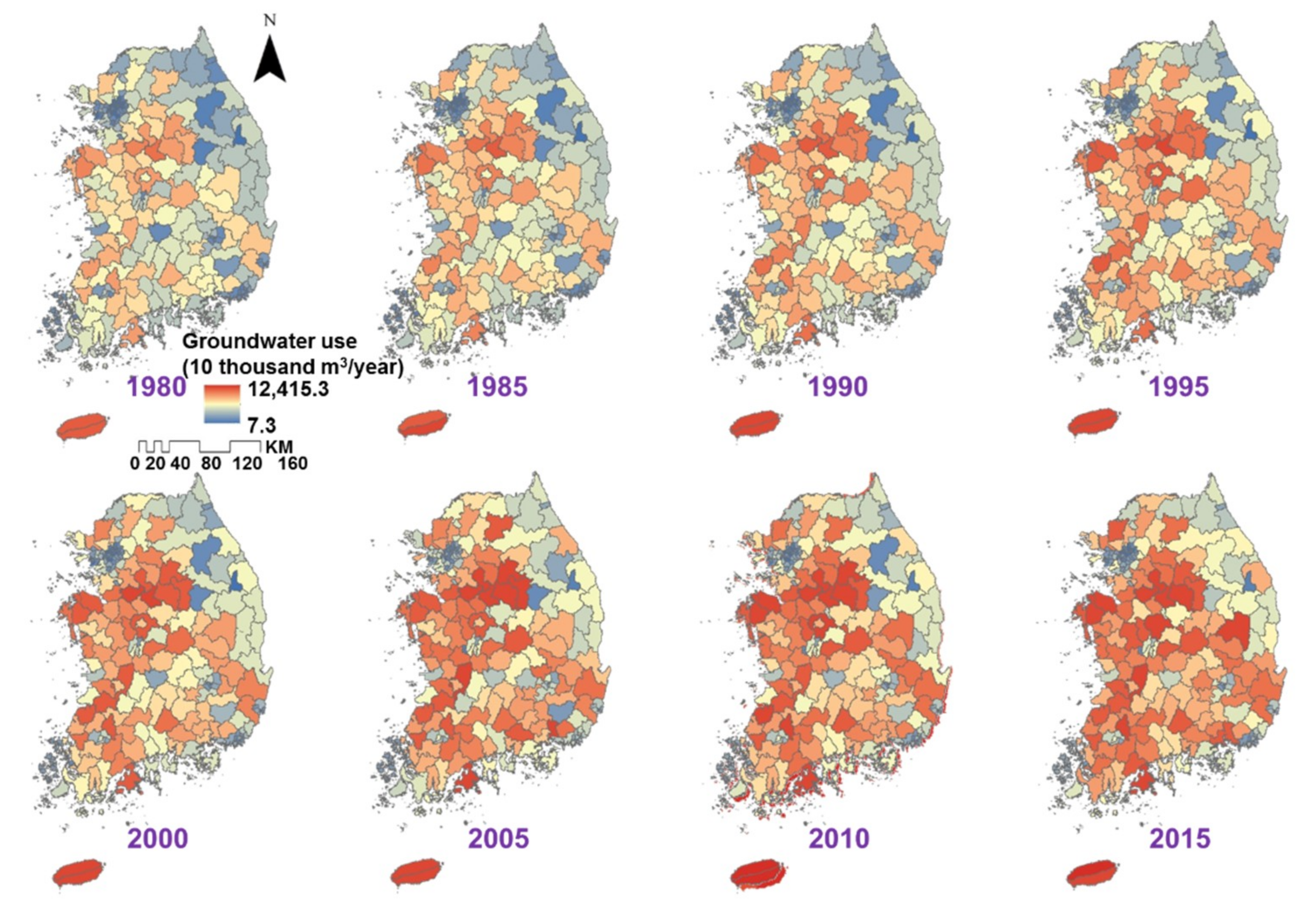
Appendix B.1. Groundwater Use (GWU)

Water enters groundwater storage mainly through infiltration and percolation, although recharging through seepage from surface water bodies can occur. The SWAT model simulates shallow aquifer and deep aquifer of a subbasin. A shallow aquifer is an unconfined aquifer that contributes to the flow in a main channel or reaches a subbasin and a deep aquifer is a confined aquifer. The water entering a deep aquifer is assumed to contribute to the streamflow somewhere outside of a given watershed [58]. The Drying Stream Assessment Tool via grid-based data mining and Water Flow Tracking (DrySAT-WFT) model uses the groundwater algorithm of the SWAT model. However, as the aquifer examined consists of a single layer, a pumping parameter for groundwater was added. The following equation was applied:
aqi = aqi-1 + wrchrg − Qgw − wrevap − wpump
where aqi represents the amount of water stored in the aquifer on day i (mm), aqi-1 represents the amount of water stored in the aquifer on day i − 1 (mm), wrchrg represents the amount of water recharge entering the aquifer on day i (mm), Qgw represents the groundwater flow or base flow (mm), wrevap represents the amount of water moving into the soil zone in response to water deficiencies on day i (mm), and wpump represents the amount of water removed from the aquifer by GWU on day i (mm).
Over the past 40 years (1976 to 2015), GWU has constantly increased (Figure A1). The average annual GWU values for the 1990s and 2010s reached 2,101,130,250 m3 year−1 and 3,658,132,125 m3 year−1, respectively. GWU increased by 74.1% from the 1990s (1980–1995) to the 2010s (2000–2015).
Figure A1. Distribution map of groundwater use (GWU) for different regions from 1980 to 2015 in the study area in five-year intervals.
Water 11 00477 g0a1

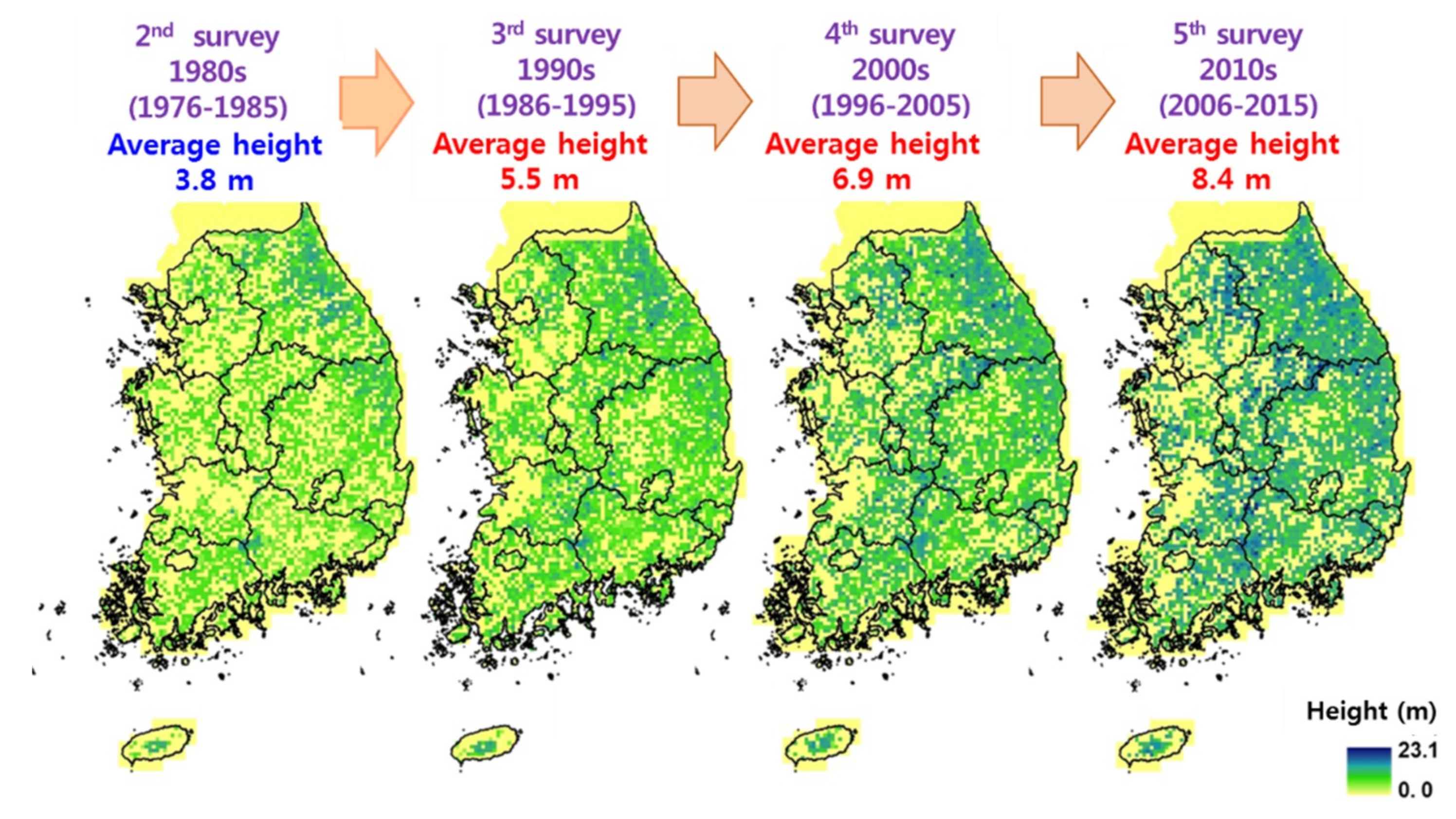
Appendix B.2. Forest Height (FH)

The model uses the Penman-Monteith (PM) method to estimate ET based on solar radiation, air temperature, relative humidity and wind speed. The PM equation combines components that account for energy needed to sustain evaporation, the strength of the mechanism required to remove water vapor and the aerodynamic and surface resistance terms. In the equation, aerodynamic resistance is influenced by sensible heat, vapor transfer and forest height (FH). The aerodynamic resistance ( γ a ) equation is as follows [45]:
γ a = ln [ ( z w d ) / z om ] ln [ ( z p d ) / z ov ] k 2 u z
Z om   =   0.123 × h c     h c 200   cm
Z om = 0.123 × h c     h c > 200   cm
Z ov = 0.1 × Z om
d   =   2 / 3 × h c     h c > 200   cm
where z w represents the height of the wind speed measurement (cm), z p represents the height of the humidity (psychrometer) and temperature measurements (cm), d represents the zero plane displacement of the wind profile (cm), z om represents the roughness length for momentum transfer (cm), z ov represents the roughness length for vapor transfer (cm), k represents the von Karman constant, u z represents the wind speed at height z w (m s−1) and h c represents the mean height of the plant canopy. Therefore, the DrySAT-WFT model used for the calculation of aerodynamic resistance was modified to apply the changes in FH from past to present. This study used forest type maps from the second to fifth surveys. Then, the forest densities and heights for each region were converted into grids of 1 km by 1 km covering South Korea (Figure A2).
Figure A2. Distribution map of forest heights (FHs) from 1976 to 2015 in the study area.
Water 11 00477 g0a2

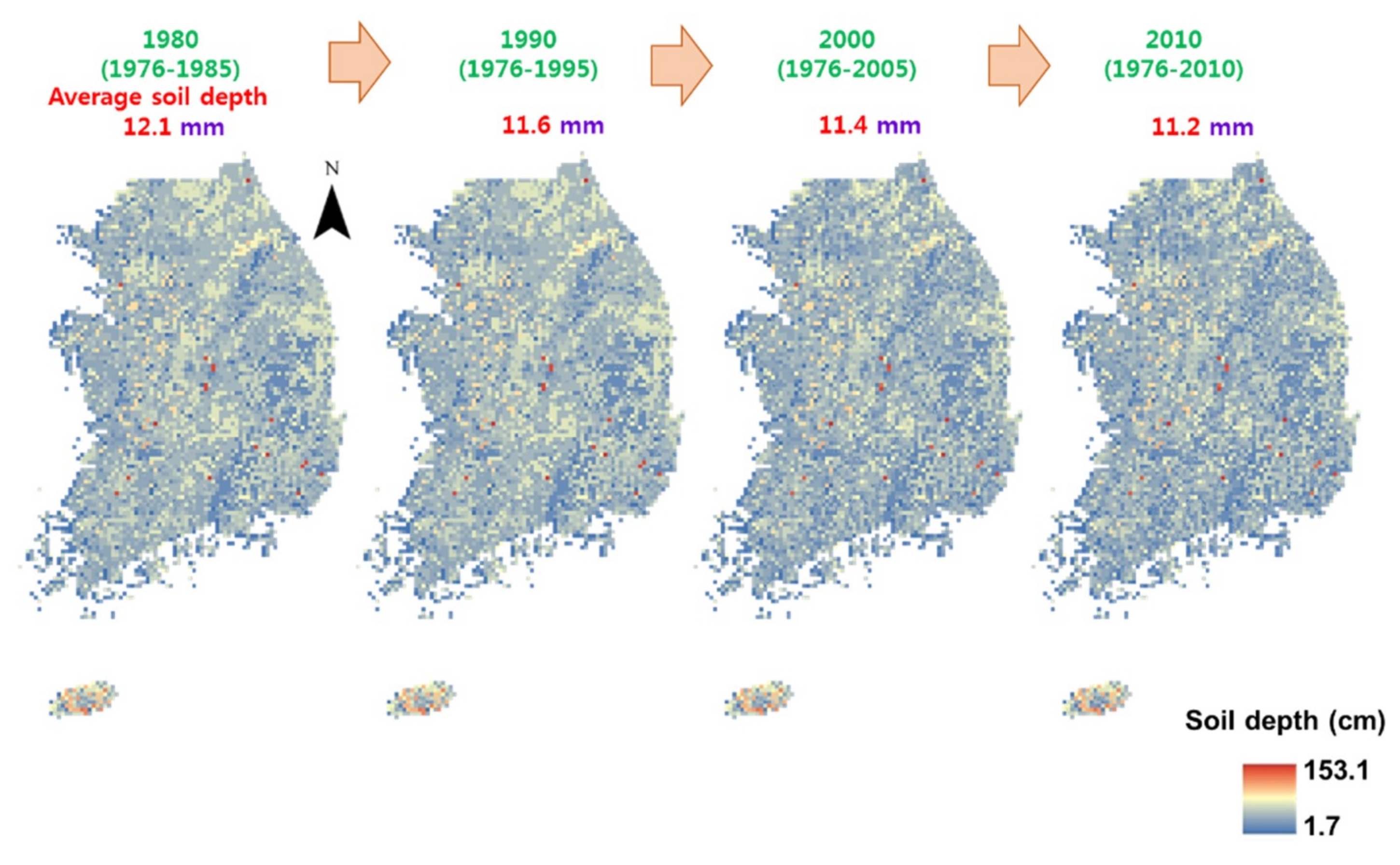
Appendix B.3. Soil Depth (SD)

SD affects the soil porosity and water content by percolation and can generate distinct transpiration rates. Variations in SD and total volumes of soil water stored in the soil profile at the end of the wet season spur differences in the SM content and transpiration rates [39]. The DrySAT-WFT model modifies the soil ET module with the SWAT model equations as follows:
E a   = E can   = E o
R INT ( f )   =   R INT ( i )   E can
E o   = E o   E can
E t   =   E o × LAI 3.0
E t   = E o
E s   = E o × cov sol
E s   =   min [ E s ,   E o · E s E s + E t ]
E soil , z   = E s × z z + exp ( 2.374 0.00713 × z )
where E a represents the actual amount of ET occurring in the watershed on a given day (mm), E can represents the amount of evaporation from free water in the canopy on a given day (mm), E o represents the potential ET on a given day (mm), E o represents the potential ET adjusted for the evaporation of free water in the canopy (mm), LAI represents the leaf area index, cov sol represents the soil cover index, R INT ( i ) represents the initial amount of free water held in the canopy on a given day (mm), R INT ( f ) represents the final amount of free water held in the canopy on a given day (mm), E s represents the maximum level of sublimation/soil evaporation occurring on a given day (mm), E soil , z represents the evaporative demand measured at depth z (mm), E s represents the maximum level of soil water evaporation occurring on a given day (mm), and z represents the depth below the surface.
Figure A3 shows the changes in SD measured by decade. Over the past 40 years (1976 to 2015), the SD has constantly decreased. The average SD values for the 1980s (1976–1985), 1990s (1986–1995), 2000s (1996–2005), and 2010s (2006–2015) were measured as 12.1, 11.6, 11.4, and 11.2 mm, respectively. Compared to the SD for the 1980s, the values decreased by 0.52 mm (4.3%), 0.67 mm (5.5%), and 0.82 mm (6.8%) in the 1990s, 2000s, and 2010s, respectively.
Figure A3. Soil depth (SD) distribution map for the study area.
Water 11 00477 g0a3

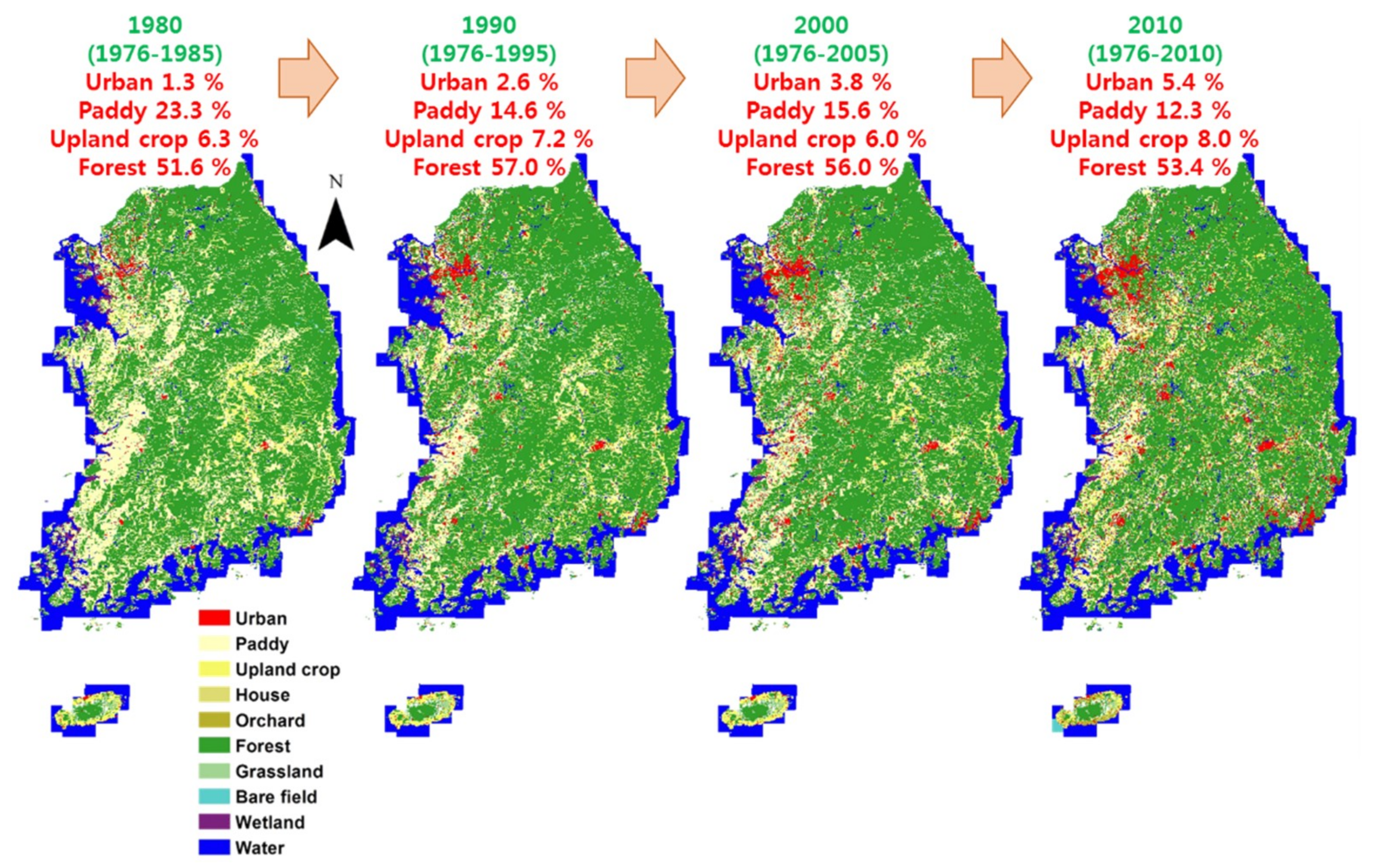
Appendix B.4. Land Use (LU)

The impacts of LU/land cover (LC) changes on the subsurface components of the hydrologic cycle are less understood, particularly with respect to groundwater recharge. Subsurface impacts can be significant. Groundwater is one of the largest freshwater resource in Earth’s. Because of this, the reduced reliability of the surface water supply may result in an increased reliance on groundwater [59]. The above algorithm defines canopy heights according to different LUs. Such differences affect the levels of aerodynamic resistance. Therefore, the DrySAT-WFT model is modified to apply LU changes to each cell. The model reads all LU data from list files.
LUs observed in 1980 are as follows: 51.6% forests, 23.3% rice paddy farmlands, 6.3% upland croplands, and 1.3% urban areas. LUs observed in 1990 are as follows: 57.0% forests, 14.6% rice paddy farmlands, 7.2% upland croplands, and 2.6% urban areas. LUs observed in 2000 are as follows: 56.0% forests, 15.6% rice paddy farmlands, 6.0% upland croplands, and 3.8% urban areas. LUs observed in 2010 are as follows: 53.4% forests, 12.3% rice paddy farmlands, 8.0% upland croplands, and 5.4% urban areas (Figure A4).
Figure A4. Distribution map of land uses (LUs) from 1976 to 2015 in the study area.
Water 11 00477 g0a4

Appendix B.5. Road Network (RN)

Road networks also have the potential to affect hydrological processes by intercepting subsurface flows along road cuts and transforming them into surface runoff when conditions are favorable [60,61,62]. Intercepted subsurface flows have been frequently used to explain hydrological regime changes (see [63,64,65,66,67,68]), suggesting that their occurrence is unexceptional. Few studies have attempted to quantify the relative contributions of overland flows to road runoff [62,63,64,65,66,67,68]. Negishi et al. [68] reported that the runoff ratio of an intercepted subsurface decreases by 40% due to the presence of a road cut. Thus, the DrySAT-WFT model includes the reduction ratio for the subsurface as follows:
Qtot = Qsurf + (roadreduction × Qmid) + Qsub
where Q tot represents the total runoff (mm), Q surf represents the surface flow (mm), road reduction represents the reduction ratio of the subsurface by the road cut, Q mid represents the subsurface flow (mm), and Q sub represents the groundwater flow (mm).
Th RN density changes in the total road length by decade intervals. From 1976 to 2015, road lengths have constantly increased. Total road lengths in the 1980s (1976–1985), 1990s (1986–1995), 2000s (1996–2005), and 2010s (2006–2015) were measured at 13,256.1 km, 15,948.9 km, 21,033.9 km, and 22,850.6 km, respectively. Relative to the total road length measured for the 1980s, the total road length increased by 2692.9 km (20.3%), 7777.8 km (58.7%), and 9594.5 km (72.4%) in the 1990s, 2000s, and 2010s, respectively.

References

  1. Lake, P. Disturbance, patchiness, and diversity in streams. J. N. Am. Benthol. Soc. 2000, 19, 573–592. [Google Scholar] [CrossRef]
  2. Matthews, W.J.; Marsh-Matthews, E. Effects of drought on fish across axes of space, time and ecological complexity. Freshw. Biol. 2003, 48, 1232–1253. [Google Scholar] [CrossRef]
  3. Dekar, M.P.; Magoulick, D.D. Factors affecting fish assemblage structure during seasonal stream drying. Ecol. Freshw. Fish 2007, 16, 335–342. [Google Scholar] [CrossRef]
  4. Sophocleous, M. Managing water resources systems: Why “safe yield” is not sustainable. Groundwater 1997, 35, 561. [Google Scholar] [CrossRef]
  5. Rural Research Institute. A Study on Causative Factors of Drying Streams in Rural Area; Rural Research Institute: Tehran, Iran, 2006. [Google Scholar]
  6. K-water. Establishment of Quantitative Soundness Evaluation System in National Rivers (Korean); K-water: Seoul, South Korea, 2008. [Google Scholar]
  7. Lee, Y.G. Estimation of Spatial Evapotranspiration for South Korea by Modifying Meso-Scale SEBAL Model. Master’s Thesis, Konkuk University, Seoul, South Korea, 2016. [Google Scholar]
  8. Jung, K.S.; Cho, H.S.; Kim, J.Y.; Shim, M.P. Analysis of drying streams characteristics using a GIS. J. Korea Water Resour. Assoc. 2003, 36, 1083–1095. [Google Scholar] [CrossRef]
  9. Ministry of Science and ICT. Technology of Sustainable Surfacewater Development (Korean); Ministry of Science and ICT: Gwacheon, Gyeonggi-do, South Korea, 2003. [Google Scholar]
  10. Barron, O.; Barr, A.; Donn, M.J. Effect of urbanisation on the water balance of a catchment with shallow groundwater. J. Hydrol. 2013, 485, 162–176. [Google Scholar] [CrossRef]
  11. Kim, S.J.; Chae, H.S.; Yoo, C.S.; Shin, S.C. Stream discharge prediction via a grid based soil water routing with paddy fields 1. Jawra J. Am. Water Resour. Assoc. 2003, 39, 1143–1155. [Google Scholar] [CrossRef]
  12. Kim, S.J.; Kwon, H.J.; Park, G.A.; Lee, M.S. Assessment of land-use impact on streamflow via a grid-based modelling approach including paddy fields. Hydrol. Process. 2005, 19, 3801–3817. [Google Scholar] [CrossRef]
  13. Farokhnia, A.; Morid, S.; Byun, H.R. Application of global SST and SLP data for drought forecasting on Tehran plain using data mining and ANFIS techniques. Theor. Appl. Climatol. 2011, 104, 71–81. [Google Scholar] [CrossRef]
  14. Cho, Y.A. Watershed water quality evaluation model using data mining as an alternative to physical watershed models. Water Sci. Technol. Water Supply 2016, 16, 703–714. [Google Scholar] [CrossRef]
  15. Granata, F.; Gargano, R.; De Marinis, G. Support Vector Regression for Rainfall-Runoff Modeling in Urban Drainage: A Comparison with the EPA’s Storm Water Management Model. Water 2016, 8, 69. [Google Scholar] [CrossRef]
  16. Granata, F.; Saroli, M.; de Marinis, G.; Gargano, R. Machine Learning Models for Spring Discharge Forecasting. Geofluids 2018, 2018, 8328167. [Google Scholar] [CrossRef]
  17. Intaraprasong, T.; Zhan, H. A general framework of stream–aquifer interaction caused by variable stream stages. J. Hydrol. 2009, 373, 112–121. [Google Scholar] [CrossRef]
  18. Bakker, M.; Anderson, E.I. Steady flow to a well near a stream with a leaky bed. Groundwater 2003, 41, 833–840. [Google Scholar] [CrossRef]
  19. Theis, C. The effect of a well on the flow of a nearby stream. Trans. Am. Geophys. Union 1941, 22, 734–738. [Google Scholar] [CrossRef]
  20. Glover, R.E.; Balmer, G.G. River depletion resulting from pumping a well near a river. Trans. Am. Geophys. Union 1954, 35, 468–470. [Google Scholar] [CrossRef]
  21. Hantush, M.S. Wells near streams with semipervious beds. J. Geophys. Res. 1965, 70, 2829–2838. [Google Scholar] [CrossRef]
  22. Jenkins, C.T. Techniques for computing rate and volume of stream depletion by Wells. Groundwater 1968, 6, 37–46. [Google Scholar] [CrossRef]
  23. Hunt, B. Unsteady stream depletion from ground water pumping. Groundwater 1999, 37, 98–102. [Google Scholar] [CrossRef]
  24. Hunt, B. Unsteady stream depletion when pumping from semiconfined aquifer. J. Hydrol. Eng. 2003, 8, 12–19. [Google Scholar] [CrossRef]
  25. Hunt, B. Stream depletion for streams and aquifers with finite widths. J. Hydrol. Eng. 2008, 13, 80–89. [Google Scholar] [CrossRef]
  26. Landsberg, J.J.; Gower, S.T. Applications of Physiological Ecology to Forest Management; Academic Press: San Diego, CA, USA, 1997. [Google Scholar]
  27. Langford, K.J. Change in yield of water following a bushfire in a forest of Eucalyptus regnans. J. Hydrol. 1976, 29, 87–114. [Google Scholar] [CrossRef]
  28. Hornbeck, J.W.; Adams, M.B.; Corbett, E.S.; Verry, E.S.; Lynch, J.A. Long-term impacts of forest treatments on water yield: A summary for northeastern USA. J. Hydrol. 1993, 150, 323–344. [Google Scholar] [CrossRef]
  29. Cornish, P.M. The effects of logging and forest regeneration on water yields in a moist eucalypt forest in New South Wales, Australia. J. Hydrol. 1993, 150, 301–322. [Google Scholar] [CrossRef]
  30. Vertessy, R.A.; Watson, F.G.R.; O′Sullivan, S.K. Factors determining relations between stand age and catchment water balance in mountain ash forests. For. Ecol. Manag. 2001, 143, 13–26. [Google Scholar] [CrossRef]
  31. Vertessy, R.A.; Benyon, R.G.; O’Sullivan, S.K.; Gribben, P.R. Relationships between stem diameter, sapwood area, leaf area and transpiration in a young mountain ash forest. Tree Physiol. 1995, 15, 559–568. [Google Scholar] [CrossRef] [PubMed]
  32. Vertessy, R.A.; Hatton, T.J.; Reece, P.; O’Sullivan, S.K.; Benyon, R.G. Estimating stand water use of large mountain ash trees and validation of the sap flow measurement technique. Tree Physiol. 1997, 17, 747–756. [Google Scholar] [CrossRef] [PubMed] [Green Version]
  33. Jayasuriya, M.D.A.; Dunn, G.; Benyon, R.; O’Shaughnessy, P.J. Some factors affecting water yield from mountain ash (Eucalyptus regnans) dominated forests in South-East Australia. J. Hydrol. 1993, 150, 345–367. [Google Scholar] [CrossRef]
  34. Köstner, B.M.M.; Schulze, E.D.; Kelliher, F.; Hollinger, D.; Byers, J.; Hunt, J.; McSeveny, T.; Meserth, R.; Weir, P. Transpiration and canopy conductance in a pristine broad-leaved forest of Nothofagus: An analysis of xylem sap flow and eddy correlation measurements. Oecologia 1992, 91, 350–359. [Google Scholar] [CrossRef] [PubMed]
  35. Antrop, M. Landscape change and the urbanization process in Europe. Landsc. Urban Plan. 2004, 67, 9–26. [Google Scholar] [CrossRef]
  36. Haase, D. Effects of urbanisation on the water balance – a long-term trajectory. Environ. Impact Assess. Rev. 2009, 29, 211–219. [Google Scholar] [CrossRef]
  37. Trinh, D.G.; Chui, T.F.M. Assessing the hydrologic restoration of an urbanized area via an integrated distributed hydrological model. Hydrol. Earth Syst. Sci. 2013, 17, 4789–4801. [Google Scholar] [CrossRef] [Green Version]
  38. Tromp-van Meerveld, H.J.; McDonnell, J.J. On the interrelations between topography, soil depth, soil moisture, transpiration rates and species distribution at the hillslope scale. Adv. Water Resour. 2006, 29, 293–310. [Google Scholar] [CrossRef]
  39. Ahn, S.R.; Kim, S.J. Assessment of climate change impacts on the future hydrologic cycle of the Han river basin in South Korea using a grid-based distributed model. Irrig. Drain. 2016, 65, 11–21. [Google Scholar] [CrossRef]
  40. Neitsch, S.L.; Arnold, J.G.; Kiniry, J.R.; Williams, J.R. Soil and Water Aseessment Tool (SWAT) Theoretical Documentation Version 2009. Texas Water Reosurces Institute Technical Report No. 406; Texas A&M University: College Station, TX, USA, 2011. [Google Scholar]
  41. Beven, K. On subsurface stormflow: Predictions with simple kinematic theory for saturated and unsaturated flows. Water Resour. Res. 1982, 18, 1627–1633. [Google Scholar] [CrossRef]
  42. Bo, X.; Qing-Hai, W.A.N.G.; Jun, F.; Feng-Peng, H.A.N.; Quan-Hou, D.A.I. Application of the SCS-CN model to runoff estimation in a small watershed with high spatial heterogeneity. Pedosphere 2011, 21, 738–749. [Google Scholar]
  43. De Winnaar, G.; Jewitt, G.P.W.; Horan, M. A GIS-based approach for identifying potential runoff harvesting sites in the Thukela River basin, South Africa. Phys. Chem. Earth 2007, 32, 1058–1067. [Google Scholar] [CrossRef]
  44. Mishra, S.K.; Pandey, R.P.; Jain, M.K.; Singh, V.P. A rain duration and modified AMC-dependent SCS-CN procedure for long duration rainfall-runoff events. Water Resour. Manag. 2008, 22, 861–876. [Google Scholar] [CrossRef]
  45. Sloan, P.G.; Moore, I.D. Modeling subsurface stormflow on steeply sloping forested watersheds. Water Resour. Res. 1984, 20, 1815–1822. [Google Scholar] [CrossRef] [Green Version]
  46. Grismer, M.E.; Orang, M.; Snyder, R.; Matyac, R. Pan evaporation to reference evapotranspiration conversion methods. J. Irrig. Drain. Eng. 2002, 128, 180–184. [Google Scholar] [CrossRef]
  47. Penman, H.L. Natural evaporation from open water, bare soil and grass. Proc. R. Soc. Lond. A 1948, 193, 120–145. [Google Scholar]
  48. Hammer, G.L.; Goyne, P.J. Determination of regional strategies for sunflower production. In Proceedings of the International Sunflower Conference Surfers paradise, Surfers Paradise, Queensland, 14–18 March 1982; pp. 48–52. [Google Scholar]
  49. Jones, C.A.; Kiniry, J.R.; Dyke, P.T. CERES-Maize: A Simulation Model of Maize Growth and Development; Texas A&M University Press: College Station, TX, USA, 1986. [Google Scholar]
  50. Ministry of Land, Infrastructure, and Transport (MLIT). A Study on Evaluation and Improvement of Drying Stream (Korean); MLIT: Tokyo, Japan, 2009. [Google Scholar]
  51. Jung, C.G.; Kim, S.J. Evaluation of land use change and groundwater use impact on stream drying phenomena using a grid-based continuous hydrologic model. Paddy Water Environ. 2017, 15, 111–122. [Google Scholar] [CrossRef]
  52. Baik, J.; Choi, M. Evaluation of remotely sensed actual evapotranspiration products from COMS and MODIS at two different flux tower sites in Korea. Int. J. Remote Sens. 2015, 36, 375–402. [Google Scholar] [CrossRef]
  53. Nash, J.E.; Sutcliffe, J.V. River flow forecasting through conceptual models: Part I. A discussion of principles. J. Hydrol. 1970, 10, 283–290. [Google Scholar]
  54. Moriasi, D.N.; Arnold, J.G.; Van Liew, M.W.; Bingner, R.L.; Harmel, R.D.; Veith, T.L. Model evaluation guidelines for systematic quantification of accuracy in watershed simulations. Am. Soc. Agric. Biol. Eng. 2007, 50, 885–900. [Google Scholar] [CrossRef]
  55. Arnold, J.G.; Allen, P.M.; Bernhardt, G. A comprehensive surface-groundwater flow model. J. Hydrol. 1993, 142, 47–69. [Google Scholar] [CrossRef]
  56. Hong, W.Y.; Park, G.; Jeong, I.K.; Kim, S.J. Development of a grid-based daily watershed runoff model and the evaluation of its applicability. J. Korean Soc. Civ. Eng. 2010, 30, 459–469. [Google Scholar]
  57. Verhoef, A.; Feddes, R.A. Preliminary Review of Revised FAO Radiation and Temperature Methods Land and Water Division; FAO: Rome, Italy, 1991. [Google Scholar]
  58. Scanlon, B.R.; Reedy, R.C.; Stonestrom, D.A.; Prudic, D.E.; Dennehy, K.F. Impact of land use and land cover change on groundwater recharge and quality in the Southwestern US. Glob. Chang. Biol. 2005, 11, 1577–1593. [Google Scholar] [CrossRef]
  59. Burroughs, E.R.; Marsden, M.A.; Haupt, H.F. Volume of snowmelt intercepted by logging roads. J. Irrig. Drain. Div. Am. Soc. Civ. Eng. 1972, 98, 1–12. [Google Scholar]
  60. Megahan, W.F. Subsurface flow interception by a logging road in mountains of central Idaho. In National Symposium on Watershed in Transition; American Water Resources Association: Middleburg, VA, USA, 1972; pp. 350–356. [Google Scholar]
  61. Megahan, W.F.; Clayton, J.L. Tracing subsurface flow on roadcuts on steep, forested slopes1. Soil Sci. Soc. Am. J. 1983, 47, 1063–1067. [Google Scholar] [CrossRef]
  62. Harr, R.D.; Harper, W.C.; Krygier, J.T.; Hsieh, F.S. Changes in storm hydrographs after road building and clear-cutting in the Oregon Coast Range. Water Resour. Res. 1975, 11, 436–444. [Google Scholar] [CrossRef]
  63. King, J.G.; Tennyson, L.C. Alteration of streamflow characteristics following road construction in North Central Idaho. Water Resour. Res. 1984, 20, 1159–1163. [Google Scholar] [CrossRef]
  64. Jones, J.A.; Grant, G.E. Peak flow responses to clear-cutting and roads in small and large basins, Western Cascades, Oregon. Water Resour. Res. 1996, 32, 959–974. [Google Scholar] [CrossRef]
  65. Wemple, B.C.; Jones, J.A.; Grant, G.E. Channel network extension by logging roads in two basins, western cascades, oregon. Jawra J. Am. Water Resour. Assoc. 1996, 32, 1195–1207. [Google Scholar] [CrossRef]
  66. Jones, J.A. Hydrologic processes and peak discharge response to forest removal, regrowth, and roads in 10 small experimental basins, Western Cascades, Oregon. Water Resour. Res. 2000, 36, 2621–2642. [Google Scholar] [CrossRef] [Green Version]
  67. Wemple, B.C.; Jones, J.A. Runoff production on forest roads in a steep, mountain catchment. Water Resour. Res. 2003, 39, 1220–1228. [Google Scholar] [CrossRef]
  68. Negishi, J.N.; Sidle, R.C.; Ziegler, A.D.; Noguchi, S.; Rahim, N.A. Contribution of intercepted subsurface flow to road runoff and sediment transport in a logging-disturbed tropical catchment. Earth Surf. Process. Landf. 2008, 33, 1174–1191. [Google Scholar] [CrossRef]
Figure 1. The model structure and flow chart in this study.
Water 11 00477 g001
Figure 2. Study area of South Korea: (a) rivers and digital elevation model (DEM) and (b) locations of the streamflow and soil moisture (SM) monitoring stations and flux towers in South Korea.
Water 11 00477 g002
Figure 3. Comparison of the observed and DrySAT-WFT-simulated daily runoff during 2006–2015 at the (a) Chungju dam (CJ), (b) Soyanggang dam (SY), (c) Andong dam (AD), (d) Imha dam (IH), (e) Hapcheon dam (HC), (f) Seomjingang dam (SJ), (g) Osucheon dam (OSC), (h) Juam dam (JA), (i) Yongdam dam (YD), (j) Mihocheon dam (MHC), (k) Mareuk dam (MR), and (l) Chogang dam (CG).
Water 11 00477 g003aWater 11 00477 g003bWater 11 00477 g003c
Figure 4. Comparison graphs of the monthly results of the water budgets after applying each water loss DB: (a) total runoff (TQ), (b) evapotranspiration (ET), (c) surface runoff (SQ), (d) lateral runoff (LQ), (e) base flow (BQ) and (f) percolation (PERC).
Water 11 00477 g004aWater 11 00477 g004b
Figure 5. Distribution results of the stream drying index (SDI) and precipitation (PCP) for the periods after applying all water loss DBs (All DBs).
Water 11 00477 g005
Table 1. Description of the stream drying index (SDI) for identifying progression.
SDIStream Drying ProgressionConditionComments
1D ≤ 10Normal-
210 < D ≤ 30WeakMonitor
330 < D ≤ 50WarningMonitor carefully
450 < D ≤ 90SevereRequires short-term improvement
590 < DVery severeRequires long-term improvement
SDI = stream drying index; D = annual daily counts of less than the 10-day minimum flow (Q355, standard flow) below the normal year.
Table 2. Model calibrated parameters.
ParametersDefinitionUnitCalibrated Values
CJSYADIHHCSJYDJAOSCMHCMRCG
inf_rtSoil infiltration ratio%0.020.020.010.010.10.080.20.350.30.30.20.1
per_rtSoil percolation ratio%0.30.20.20.20.30.350.40.40.250.150.20.3
surlagSurface runoff lag coefficient-44554.53432.52.52.52
slp_lLateral flow recession curve slopedegree0.30.30.30.30.20.250.40.40.20.30.30.25
time_lLateral flow lag timeday668877654655
slp_bBaseflow recession curve slopedegree0.250.250.250.250.250.30.30.30.20.350.350.2
time_bBaseflow basin lag timeday771010778991078
CANMXMaximum canopy storagemm777755555555
Table 3. Average classified SDI accuracy of 4 and 5 grades between the DrySAT and the status survey report results from 2001 to 2010.
BasinsState Survey (Middle Watersheds)DrySAT Results (Standard Watersheds)Accuracy (%)
4 Grades5 GradesTotal4 Grades5 GradesTotal4 and 5 Grades
Han-river3/305/308/3087/25833/258120/25821/69
(10.0%)(16.7%)(26.6%)(33.7%)(12.8%)(46.5)(30.4%)
Nakdong-river10/4212/4222/4275/26540/265115/26588/124
(23.8%)(28.6%)(52.4%)(28.3%)(15.1%)(43.4)(71.0)
Geum-river4/206/2010/2064/13730/13794/13732/44
(20.0%)(30.0%)(50.0%)(46.7%)(21.9%)(68.6)(72.7%)
Seomjin-river3/103/106/1030/7310/7340/7322/32
(30.0%)(30.0%)(60.0%)(41.1%)(13.7%)(54.8)(68.8%)
Youngsan-river4/102/106/108/142/1410/1414/32
(40.0%)(20.0%)(60.0%)(57.1%)(14.3%)(71.4)(43.8%)

