Experimental Observation of Inertial Particles through Idealized Hydroturbine Distributor Geometry


Pacific Northwest National Laboratory, Richland, WA 99354, USA
*
Author to whom correspondence should be addressed.
Water 2019, 11(3), 471; https://doi.org/10.3390/w11030471
Submission received: 29 January 2019
/
Revised: 26 February 2019
/
Accepted: 26 February 2019
/
Published: 6 March 2019
(This article belongs to the Section Hydraulics and Hydrodynamics)
Abstract
:To increase and maintain existing hydropower capacity within biological performance-based regulations, predictive simulation methods are needed that can reliably estimate the risk to fish passing through flow passage routes at hydropower facilities. One of the central challenges is to validate the software capabilities for simulating the trajectories, including collisions, of inertial particles against laboratory data. In this work, neutrally buoyant spherical- and rod-shaped beads were released upstream of laboratory-scale geometries representative of the distributor of a hydroturbine. The experimental campaign involved a test matrix of 24 configurations with variations in bead geometry, collision target geometry, flow speeds, and release locations. A total of more than 10,000 beads were recorded using high-speed video cameras and analyzed using particle tracking software. Collision rates from 1–7% were observed for the cylinder geometry and rates of 1–23% were observed for the vane array over the range of test configurations.
1. Introduction
A critical challenge currently facing the development of increased hydropower capacity is the need to alleviate, mitigate, or otherwise minimize the adverse environmental impacts of hydropower to levels acceptable to regulatory agencies. The factors which influence the survival of live fish passing through a hydroelectric powerhouse have been presented in several reviews which examine fish behavior [1] and passage routes [2], as well as hydroturbine operation and design [3]. Field studies to assess the mortality rates during downstream passage have been conducted using live fish [4,5,6]. Trends in fish passage conditions have also been assessed through field studies using an autonomous sensor device deployed upstream of the turbine [7,8].
However, these methods are only possible using an installed and operational turbine. To assess the biological performance of fish passage during the turbine design phase, as well as reduce the high cost and technical difficulty associated with field testing, an efficient alternative solution to this challenge is the development of software tools that will support biologically based design, operation, and evaluation of hydroturbines and other passage routes at hydropower facilities. One existing set of computational tools developed for this purpose is the biological performance assessment (BioPA) method developed at the Pacific Northwest National Laboratory (PNNL) [9,10,11]. This approach approximates fish trajectories through a turbine by simulating the trajectories of massless particles using computational fluid dynamics (CFD). Current work is focused on increasing the physical realism of the BioPA software toolset by including the effects of particle mass and form (referred to as inertial particles).
Such simulations of fish trajectory during downstream passage require validation against laboratory observations to gain an increased confidence in the approach. Particles which are smaller than the Kolmogorov dissipation scale (low Stokes numbers) behave as tracers to the fluid flow and studies which examine such motions represent simplified approximations to the case in question. For larger particle sizes, the dynamics are affected by the particle inertia and therefore deviates from that of the surrounding fluid.
Several previous studies have experimentally quantified the acceleration statistics of LaGrangian particles in turbulent flows [12,13,14]. These data demonstrate that the stream-wise acceleration of neutrally buoyant particles with sizes greater than the Kolmogorov length scale can be quantified with a predictable shape of a probability density function. The effect of particle shape, aspect ratio, density and size on the forcing terms of non-spherical particles is investigated by [15] in the tracking of particle motion in free-fall in a vertical wind tunnel. Drag coefficients of a range of cylindrical inertial particles with varying densities, lengths and diameters were also experimentally investigated by [16] by observing the motion of particles in free-fall. Falling and rising spheres were also studied by [17] who examined and visualized the formation of vortex rings in the wakes of spheres with diameters from 2 mm to 38 mm. The motion of spherical particles, with diameters ranging from 6 mm to 24 mm, were visualized within a turbulent von Karman flow field and the frequency distribution of particle locations and velocities were presented by [18]. A pendulum test rig was set up by [19] to observe the collisions of inertial particles with a wall and measure the pressure impulses. A similar configuration was presented by [20], with results focusing on the approach and rebound trajectory of the particle.
This paper presents the experimental observation of the unrestricted motion of inertial particles toward two collision target geometries in a recirculating water flume: a single cylinder and an array of representative stay vanes and wicket gates. The distribution and trajectories of the particles were captured using high-speed video cameras and the collision rates were extracted to produce a valuable and unique data set for CFD comparison and validation.
Though the flow characteristics and passage geometries do not directly represent those encountered during fish passage through a full-scale hydroelectric powerhouse, the experimental flow and resulting particle paths are accurately measured to fully characterize the experiments presented herein. The results therefore represent a unique and useful data set to validate CFD simulations under identical conditions, in the progression toward validating full-scale fish passage simulations.
2. Materials and Methods
2.1. Experimental Design
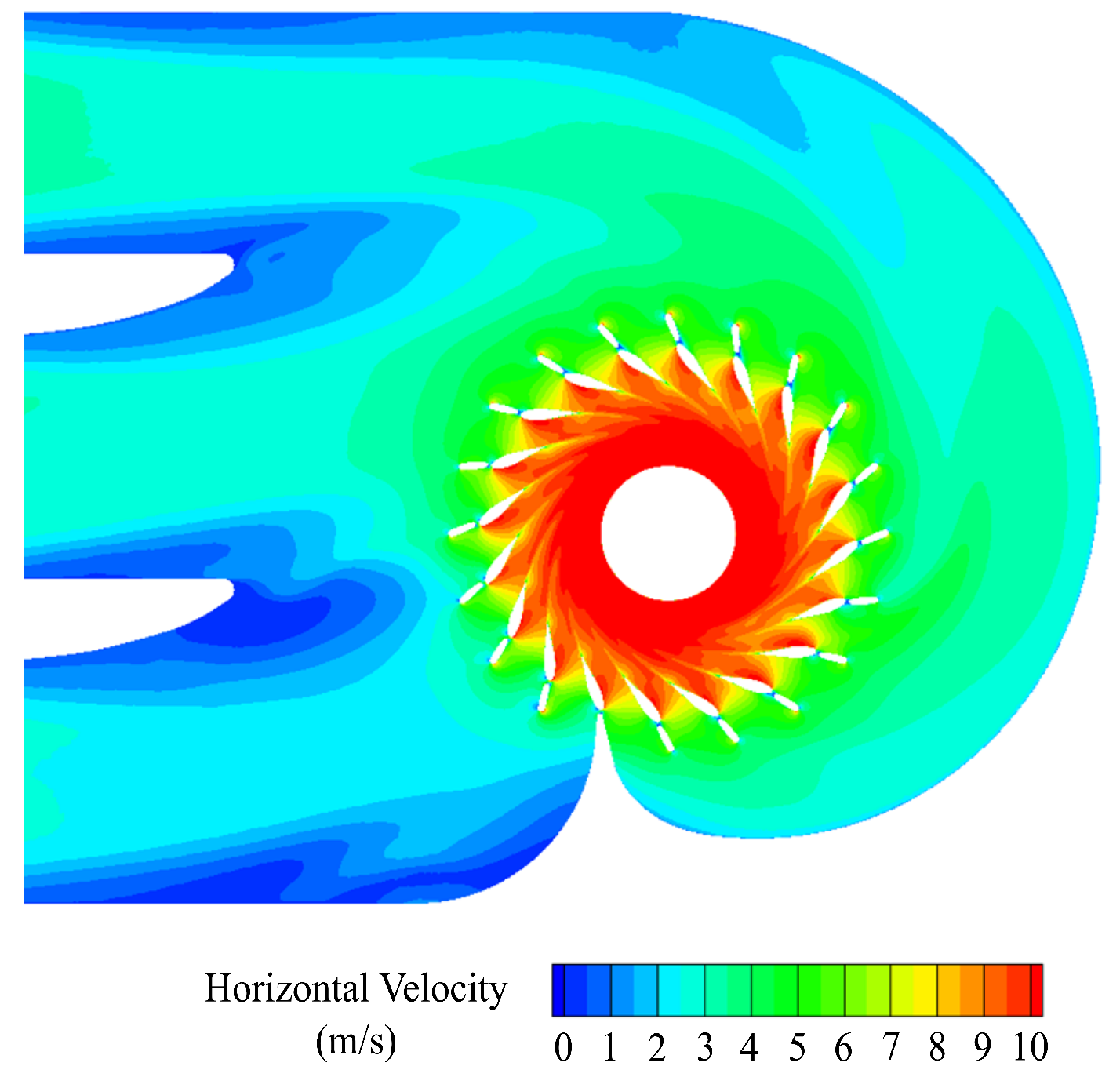
The experimental design described below was based on the configuration of the Kaplan units operating at the Ice Harbor Dam, located on the lower Snake River in Washington state, USA. The intake and distributor of one unit is shown in Figure 1, with the horizontal flow velocity overlaid, as calculated by CFD.
The laboratory experiments were conducted in the recirculating water flume at the Albrook Laboratory of Washington State University, Pullman, WA, USA [21,22]. This facility was equipped with two parallel 30 HP pumps (and has a test section measuring 0.89 m wide, 0.53 m deep and 3.75 m long). The water was pumped into the upstream end of the flume via six inlet manifolds and conditioned through one honeycomb panel and three wire mesh screens. To represent the rotating flow of the hydroturbine intake in a linear flume, the geometry of the distributor was projected from a polar coordinate system (where the vanes of the distributor are arranged in circular formation) to a linear array.
All target collision geometries were suspended below a 10 mm thick aluminum plate with locating holes drilled with CNC machining. The mounting plate was submerged by 20 mm and chamfered along the leading edge to minimize the generation of air bubbles on the underside of the plate which would complicate the particle visualization and tracking. The mounting plate was also finished with black anodizing for maximum color contrast between the beads (yellow) and the background. All test collision geometries were 500 mm long to span the distance from the aluminum mounting plate to the bottom of the flume.
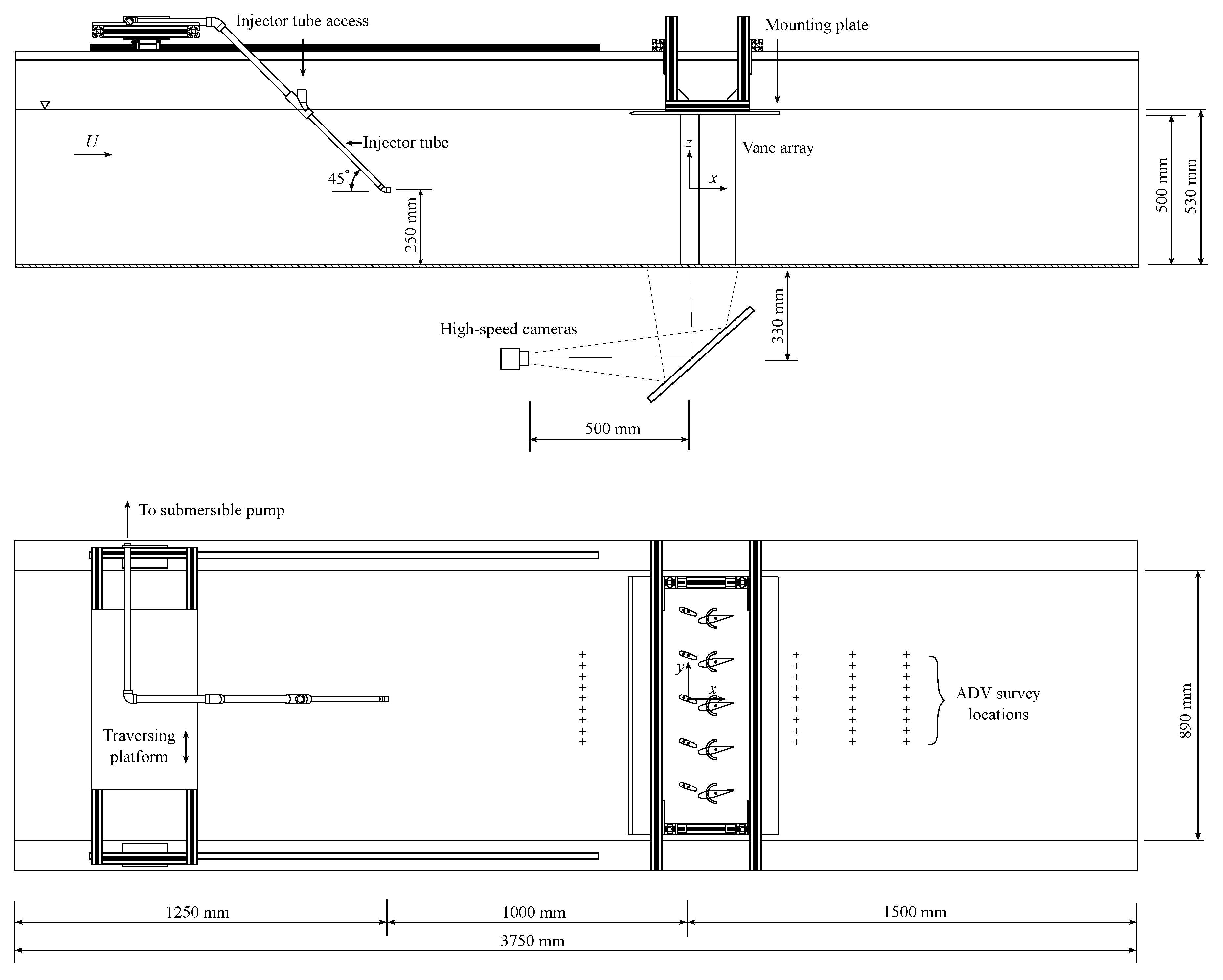
A schematic of the test section of the experimental flume is shown in Figure 2.
2.2. Experimental Variables
The following experimental variables were included in the test schedule:
2.2.1. Collision Geometry
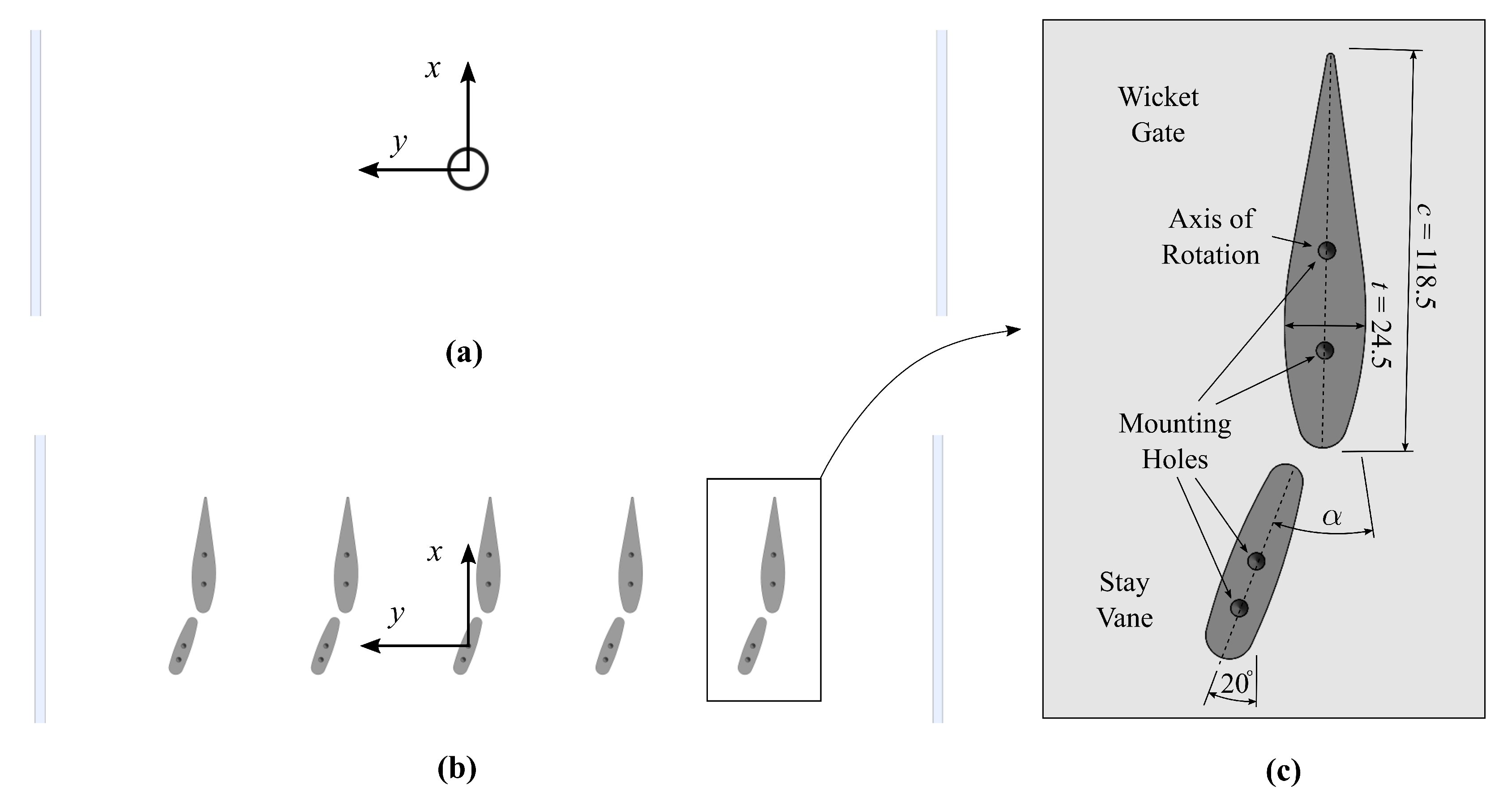
Two different geometries were placed in the path of the inertial particles and the resulting particle behavior was observed for each. Firstly, a single cylinder was selected as the simplest geometric shape for validation of the CFD and inertial particle behavior (Figure 3a). An array of 5 stay vane and wicket gate pairs was then used to represent a linear projection of the circular configuration in the hydroturbine distributor (Figure 3b). An array of vanes was used to study particle behavior between adjacent stay vane and wicket gate structures. The details of these geometries are described below.
- (a)
- CylinderThe cylinder was constructed from extruded PVC with a smooth surface finish. The center of the cylinder was used as the origin of the coordinate system used in these tests, with the x-axis in the direction of the flow, the y-axis in the transverse flow direction, and the z-axis in the vertical direction. The external diameter of the cylinder geometry was mm.
- (b)
- Stay Vane and Wicket Gate ArrayThe centroid of the central wicket gate was defined as the origin of the coordinate system used in these tests with the same coordinate system as the cylinder tests.Each hydroturbine unit at Ice Harbor Dam has a total of 20 wicket gates in the distributor which introduces rotational inertia to the flow in the scroll case, as shown in Figure 1. The incident flow direction, relative to the chord of the stay vanes, is a function of the azimuth and radial distance from the turbine axis. The distribution of incident flow directions was calculated for 3 radial locations from the leading edge of the stay vane; 100 mm, 200 mm and 300 mm. The results indicated a prevalent incident flow direction of approximately 20° relative to the stay vane chord angle. The stay vanes of the experimental tests were therefore orientated at an angle of 20° to the longitudinal axis of the flume.The cross-sectional dimensions of the stay vane and wicket gate geometry were determined using Froude scaling by a factor of 1/12 and were manufactured using CNC machining from 6061 T6 Aluminum with a black anodized finish. The resulting chord length (c) and thickness (t) of the experimental-scale wicket gate were mm and mm, respectively, as shown in Figure 3c. The harmonic mean length scale of the wicket gate (L) was calculated as mm [24]. The cross-section of each stay vane and wicket gate was constant along the length span.The harmonic mean length scale of the stay vane is approximately equal to the diameter of the cylinder geometry. The Reynolds numbers for the cylinder and vane experiments are therefore equivalent to within 4% when calculated using this length scale, such that .
2.2.2. Bead Shape
Inertial particles were fabricated from polypropylene using plastic injection molding. Calcium carbonate was added to the base material (18.1% mass fraction) to increase the density of the material to achieve a target of neutral buoyancy (specific gravity equal to unity). A yellow color concentrate was added (3.7% mass fraction) to increase the contrast of the bead against the dark background of the test geometry. Antistatic agent was also added (3.7% mass fraction) to minimize bead-to-bead interaction.
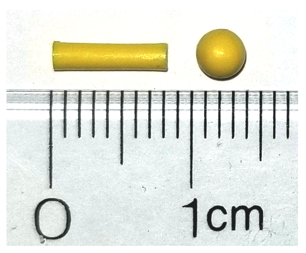
The characteristics of the beads used are described below and are shown in Figure 4.
Two particle shapes were tested, and are shown in Figure 4:
- (a)
- Rod: The rod-shaped bead geometry is based on the scaled geometry of the ‘Sensor Fish’ device [25] which is designed to represent a 100 mm long juvenile fish. The dimensions of the rod were determined using the same 1/12 Froude scaling applied to the blade geometries. This resulted in a bead with a diameter of 2.0 mm and a length of 8.0 mm.
- (b)
- Sphere: A sphere with equal volume as the rod represents a further simplification of the bead geometry by removing the geometric significance of the bead rotation upon collision. This corresponded to a diameter of 3.6 mm.
The density of a sample of 20 beads of each shape was measured using a specific gravity kit (Mineralab, Model SGK-B) and digital analytical balance (Fisher Scientific, Model AMF204AM). The mean specific gravity of the rod-shaped and spherical beads were measured to be 1.013 and 1.028, respectively.
2.2.3. Wicket Gate Angle
The angle of attack of the wicket gate is adjustable in the experimental setup within a range of ° from the stream-wise flow direction. The upper 1% and lower 1% operating conditions of Ice Harbor Dam (corresponding to the operating points with the highest and lowest flow rates which achieve a turbine efficiency within 1% of the peak efficiency for a given head) were used to define the two wicket gate angles used in these experiments. The wicket gate angle relative to the stay vane, defined by in Figure 3c, for the upper 1% and lower 1% operating condition correspond to ° and °, respectively.
2.2.4. Release Offset
The injection tube was set at two transverse locations; and . When the cylinder was installed as the collision geometry, , where D is the diameter of the cylinder. When the vane array was installed as the collision geometry, , where mm, defined by the distance between adjacent stay vane centroids.
2.2.5. Bulk Flow Speed
A low flow speed was achieved using a single pump in the recirculating plumbing of the flume and a high flow speed was achieved using two pumps in parallel. The same single pump was used for all low speed experiments for consistency of flow conditions. Taking the harmonic mean length scale of the stay vane (L) as the characteristic dimension, Reynolds numbers () corresponding to the low and high flow speeds explored in these tests were and , respectively, where , U is the mean bulk flow speed and is the kinematic viscosity of water. A more detailed characterization of the water velocity at each flow speed is presented in the following subsection.
The test matrix of the five experimental variables described above is presented in Table 1. The test numbers are used to refer to specific combinations of test variables throughout the remainder of the article.
2.3. Velocity Characterization
The flow velocity in the test section was characterized using two synchronized acoustic Doppler velocimeters (ADVs). Nortek Vectrino ADVs with Vectrino+ firmware were used for all velocity measurements described herein [26].
Each ADV was installed with a downward-looking head on a gantry system that was aligned with the Cartesian axes of the test tank shown in Figure 2. Preliminary characterization of the incident flow was performed by measuring the flow velocity in vertical transects at the center of the flume () and transverse transects at mid-depth (). This process showed the mean vertical and transverse velocity profile to be constant to within 6% of the mean flow speed within the range of and .
The flume was seeded using fine natural sediment particles with a mean diameter of 3.5 m. This seeding material was selected in preference to typical glass microsphere products because the tank drain discharged into a waterway without sufficient filtration to remove non-biodegradable material of that scale. Neutral buoyancy of the seeding particles was achieved by mixing the sediment particles with fresh water in a settling tank, allowing the suspended particles to settle for a period of 300 s. Any buoyant material was removed from the surface of the settling tank and then the seeded water was decanted from the mid-portion of the tank. Sufficient seeding of the tank water was verified by the ADV correlation metric consistently exceeding a value of 90% [27].
While the mean velocity can be determined from sampling periods of less than 60 s, higher order velocity metrics such as turbulence velocities require data acquisitions with a significantly longer duration [28]. For each characterization acquisition, the ADV was set to collect data at 100 Hz for a period of 5 min, with a transmit length of 1.2 mm and a nominally cylindrical sampling volume with a diameter of 6.0 mm and length of 4.9 mm. A nominal velocity range of m/s was selected, which provides a measurable velocity range of 0.27 m/s and 0.94 m/s in the vertical and horizontal directions, respectively. For further information on the definition and implications of these settings refer to the Nortek User Manual [29].
While a convenient method to measure three-dimensional velocities at relatively high frequency, ADV data in its raw form is prone to contamination by several sources. Letting the longitudinal (x-direction), transverse (y-direction) and vertical (z-direction) velocity components be defined by as u, v, and w, respectively, the raw velocity for the longitudinal velocity component can be defined by Equation (1). Here U represents the time-averaged mean velocity, represents the true velocity fluctuations from the mean, and represents the inherent noise in an ADV velocity measurement.
To extract the true fluctuating velocity components, the , and terms must be isolated from the velocity signal returned by the ADV (, and ). The mean velocity component was calculated as the 5-min mean velocity and subtracted directly. The removal of the noise signal prior to the calculation of the turbulence velocity is achieved using several post-processing presented in Appendix A.
2.4. High-Speed Video Recording
All bead release experiments were recorded using dual high-speed cameras to observe the trajectory of the beads on either side of the target collision geometry. The cameras used were monochrome Photron FASTCAM Mini UX50 [30], with a synchronized frame rate of 500 fps and recording time of 8.74 s at 1280 × 1024 pixel resolution. The subject distance increased to a distance greater than the vertical space available underneath the flume using a mirror mounted at 45°, as shown in Figure 2. Adjustable LED lighting was used from several source locations to create optimal subject illumination and contrast with dark background colors.
Footage of a calibration rig was recorded at the beginning of every test run to allow the pixel/mm scale factor to be determined for subsequent particle tracking analysis.
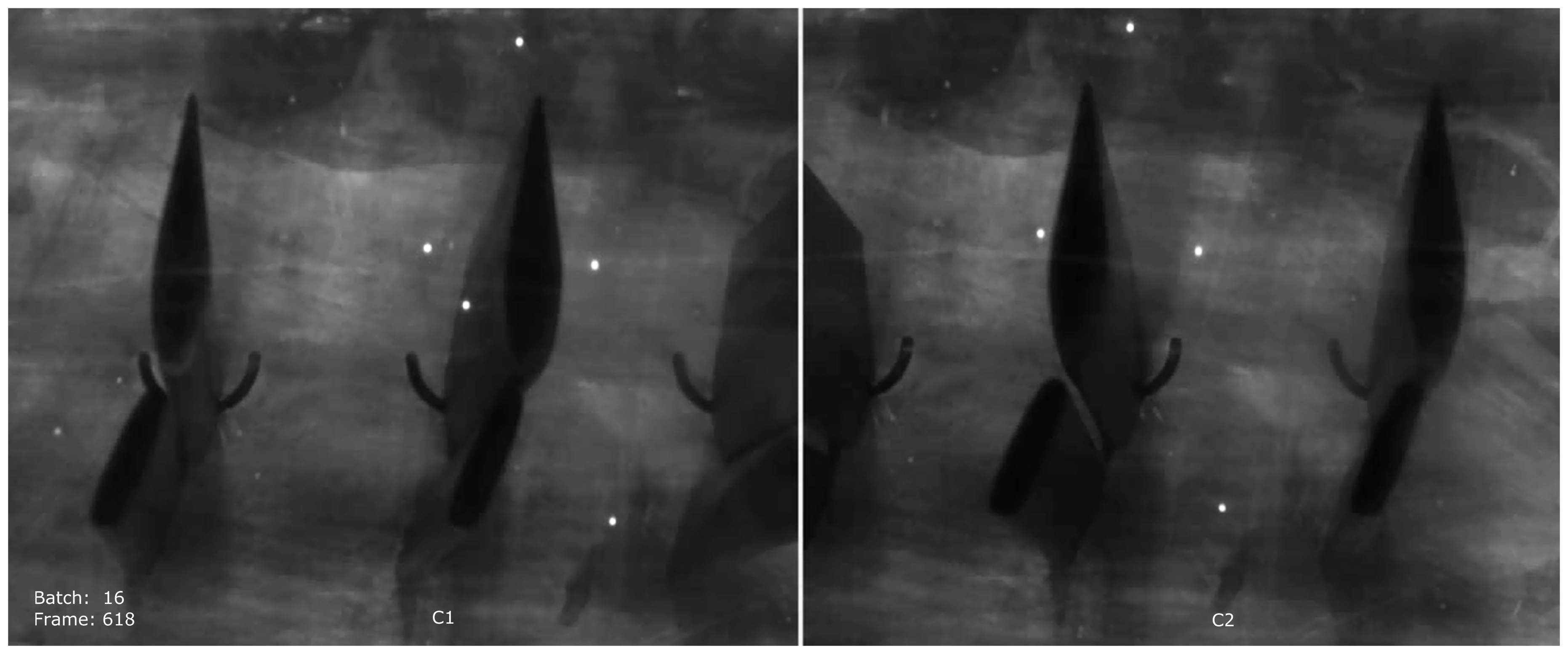
A hand-held start trigger was used to begin recording as the beads approached the field of view (FOV) such that the beads passed through the FOV within the available recording time. The video footage was clipped at the beginning and end of the recording to remove frames that contained zero beads. The footage was then post-processed to show the synchronous footage of both the left and right camera view for ease of video analysis, as shown in Figure 5.
2.5. Experimental Procedure
A test matrix was constructed that contained all the combination of the experimental variables discussed in Section 2.2 and is shown in Table 1.
For a finite number of N observed bead passages, the proportion of beads that exhibit a particular behavior is expected to fall within the range of , where P is the expected true proportion from observations and e is the precision in the observed rates of particle response to a specified confidence level. The precision is calculated using Equation (2), where Z is the value from standard normal distribution corresponding to desired confidence level (Z = 1.96 for 95% CI) [31].
The estimation of the 95% confidence interval for all observed rates of bead passage is calculated in this way for all results presented herein. Each of the 24 tests targeted a release of at least beads to provide an estimate error of . The number of beads considered in each of the tests ranged from due to discrepancies between the number of beads released and the number captured by high-speed camera.
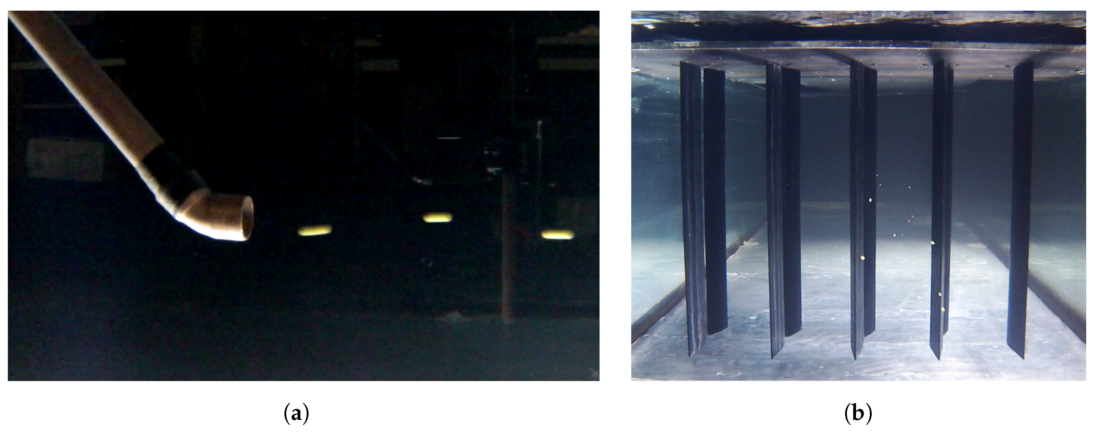
The bead injector tube was connected to a submerged pump in the tank reservoir with a mean exit velocity matched to the flow velocity of the flume. This has the benefit of accelerating the beads toward the flume velocity prior to injection and reducing the velocity deficit in the wake at the point of injection. The injection tube was constructed from 16 mm diameter copper tubing and is shown in Figure 6a.
Sets of 20 beads were suspended in 50 mL of water and inserted into the tube at the injector tube access point indicated in Figure 2. Each set of 20 beads was captured within one high-speed camera recording. A single set of released beads viewed from the downstream end of the test section is shown in Figure 6b.
A collection net was installed at the downstream end of the test section to collect the beads for reuse. This was made from fine mesh and was installed for all velocity characterization and bead release experiments such that the blockage effects were consistent throughout all tests.
The high-speed video footage was analyzed to categorize the passage of each bead according the bead passage codes convention defined by Table 2. The severity of the trajectory deviation was assessed by an observer; however, a qualitative change in trajectory was used to calibrate this assessment. This was based on the peak angular deviation from the incident flow direction where Code 1, Code 2 and Code 3 were defined by trajectory deviations of <, – and >, respectively. A collision (Code 4) was recorded for any case where the bead came in contact with the collision target object.
3. Results
3.1. Velocity Measurements
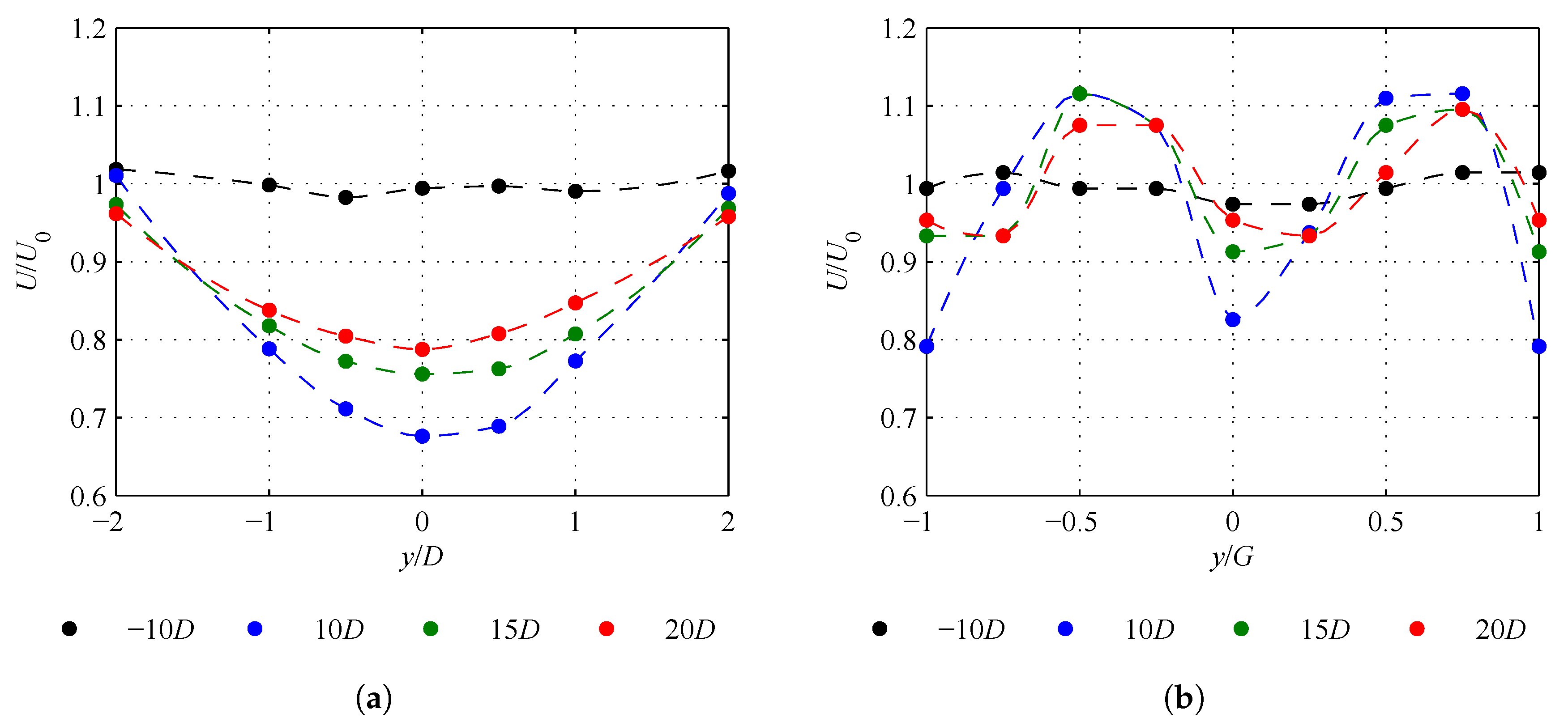
Vertical and transverse profiles of the mean flow velocity were measured at a range of stream-wise locations, both upstream and downstream of the collision object. The mean velocity profiles in the lateral direction were used to characterize the wake at several stream-wise locations, as shown in Figure 7a for the cylinder object and Figure 7b for the vane array.
The velocity metrics of the incident and wake flows were calculated using the ADV velocity measurements using the methods described in Section 2.3. The incident flow metrics for each of the flow speeds tested in this experimental campaign are presented in Table 3.
3.2. Particle Collision Results
The lateral distributions of the beads as they approached the collision object were captured using high-speed camera footage. This footage was processed at PNNL using Xcitex ProAnalyst software package to calculate the distribution of the beads at a transect of [32].
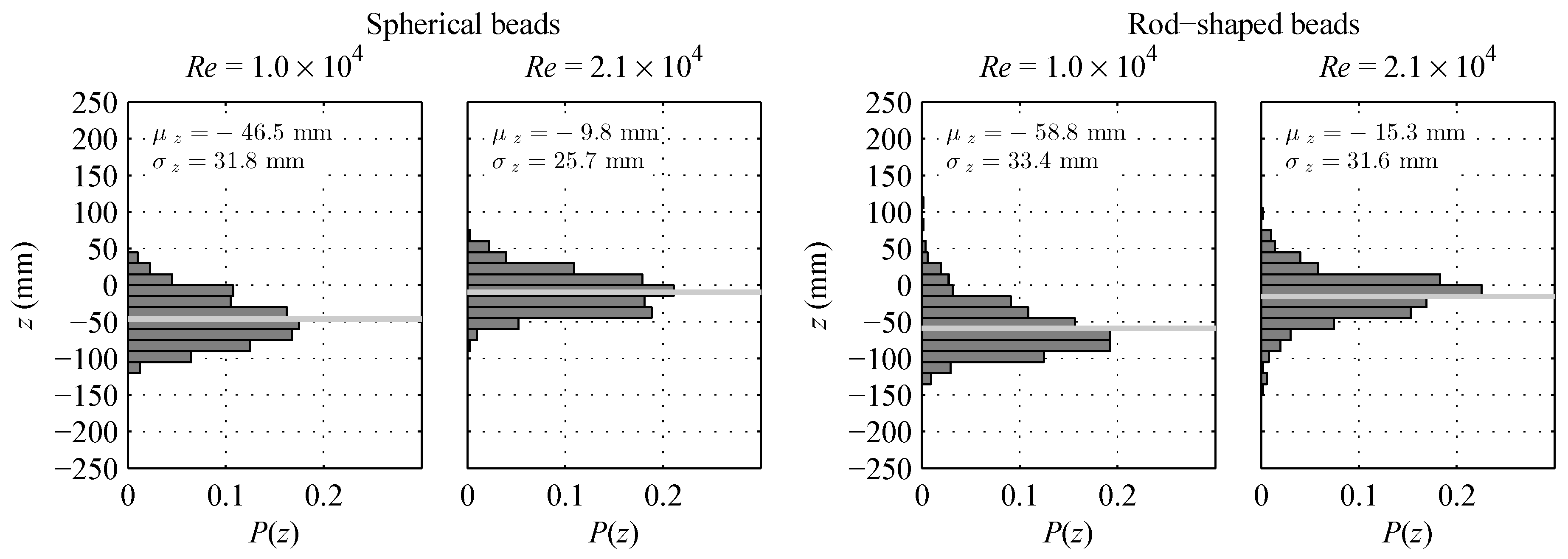
The vertical distribution of the beads, shown in Figure 8, demonstrates that all beads approached the collision objects at an elevation range of . The mean of the vertical distribution, , when was less than when . However, the vertical range of the approaching beads was within the vertical range of the velocity profile where the velocity was effectively constant (). The elevation of the beads was therefore not considered in the collision analysis.
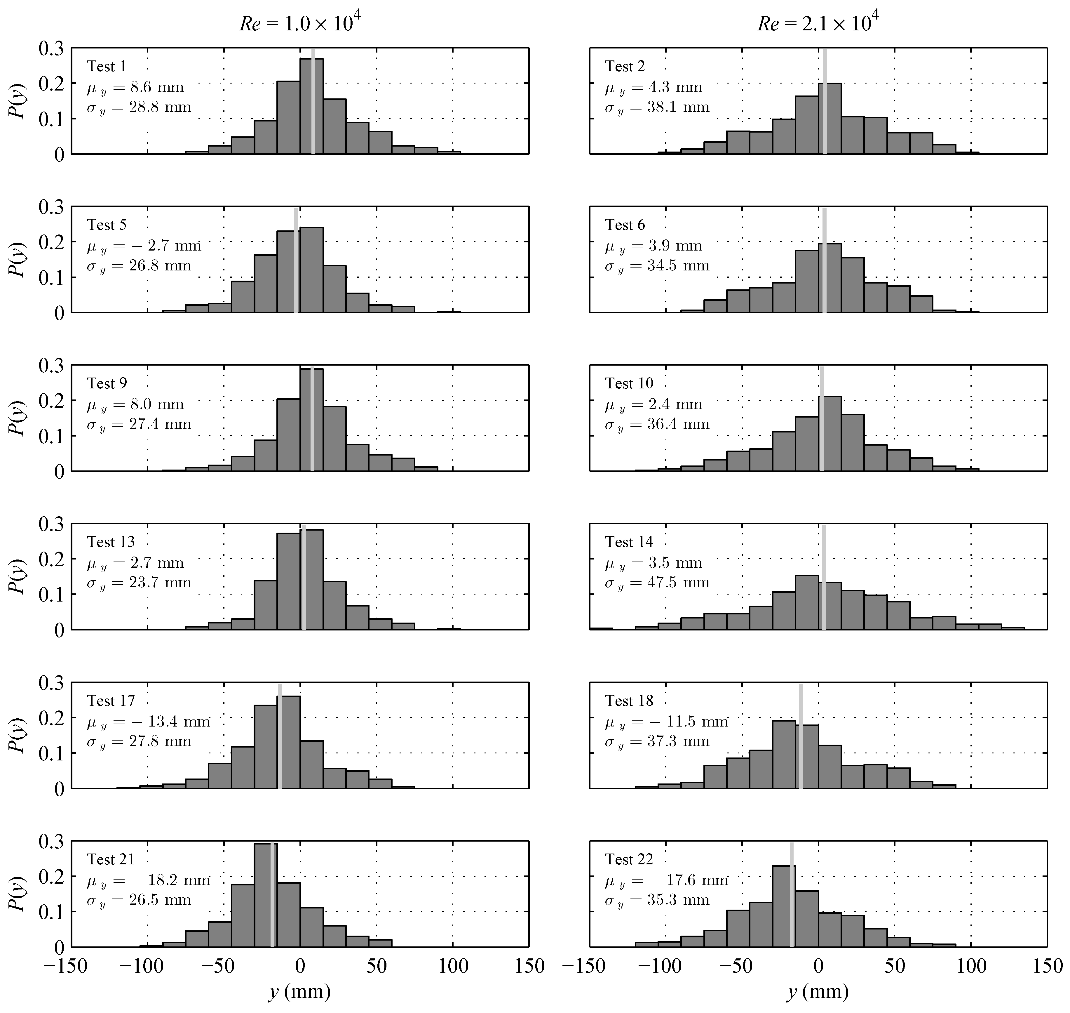
The lateral distribution of the beads, described by a mean of and standard deviation of , was affected by the geometry of the target shape and incident flow conditions. The distributions of all tests corresponding to a release location of are shown graphically in Figure 9 and the implications are discussed below.
3.2.1. Cylinder
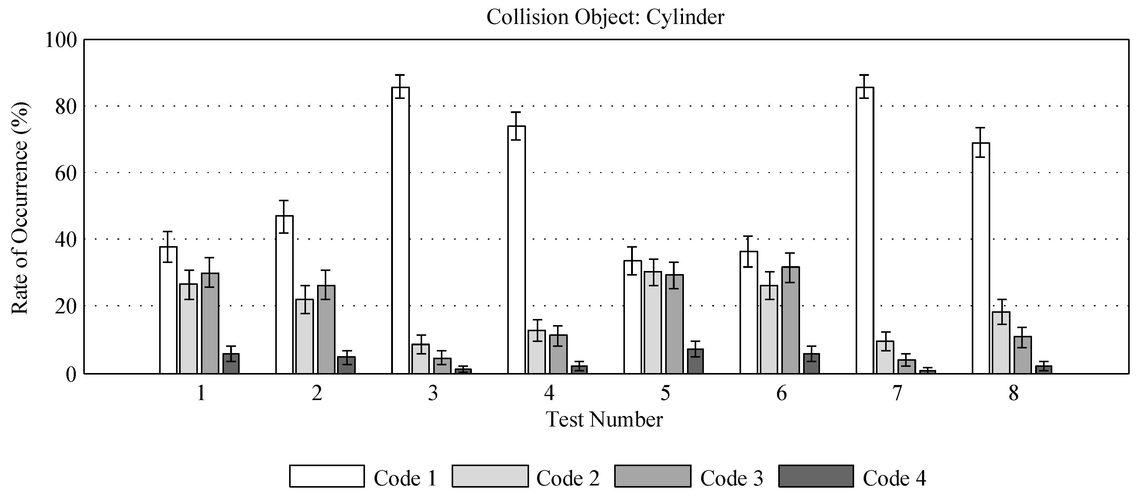
The rates of observed bead passage for each of the four codes defined in Table 2 are presented in Figure 10 for the cylinder, and discussed in the following subsections.
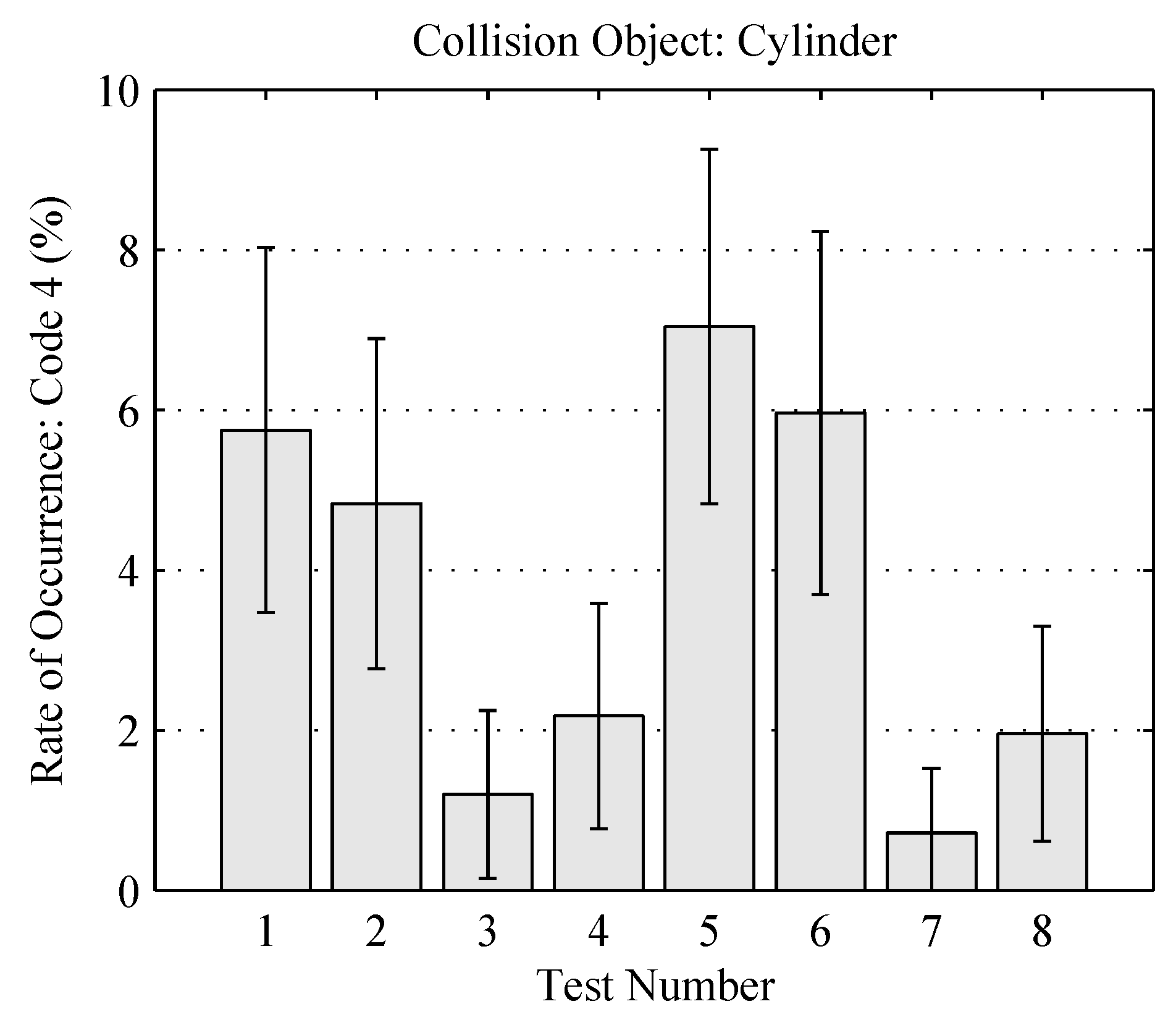
The collision rates (Code 4) for the cylinder geometry are presented in Figure 11 as a subset of the data presented in Figure 10 and will be referenced throughout this section of the article.
- Bead Shape:Tests [1–4] vs. [5–8]No significant difference between the collision rates of sphere- and rod-shaped particles were observed. Furthermore, there is no significant difference between the rate of observation of any of the bead passage codes used to describe the bead passage as a result of the bead shape. That is, the error bars of each bead passage code for the spherical bead tests overlap with the error bars for the rod-shaped bead tests with the corresponding experimental conditions.
- Release Offset:Tests [1–2] vs. [3–4] and [5–6] vs. [7–8]A significant decrease in collision rates (Code 4) was observed when release location was offset to . There is a corresponding increase in particle passage with no deviation (Code 1). This is expected as the mean of the lateral distribution is offset from the center of the cylinder by , moving many bead trajectories outside the region of influence of the cylinder.
- Flow Speed:Test 1 vs. 2, 3 vs. 4, 5 vs. 6, 7 vs. 8An increase in flow speed showed consistent trends in observed collision rates. However, the changes in collision rate in response to flow speed were not significant within the confidence intervals of this experiment.These emergent trends are best understood by recalling the increase in particle distribution as a function of increasing Reynolds Number (Figure 9). For the bead injections at , this increased bead spread causes a slight reduction in collision rate as the flow speed is increased. This is a result of a larger proportion of the beads arriving at the collision geometry at a greater distance from the cylinder axis. This effect is observed for both the spherical beads (Tests 1–2) and rod-shaped beads (Tests 5–6).For the bead injections at , the opposite trend was observed, with collision rates increasing as a function of flow speed. In this case, the increase in particle distribution allowed a greater number of beads to disperse over the lateral offset distance to collide with the cylinder geometry. Again, this effect is observed for both the spherical beads (Tests 3–4) and rod-shaped beads (Tests 7–8).
3.2.2. Vane Array
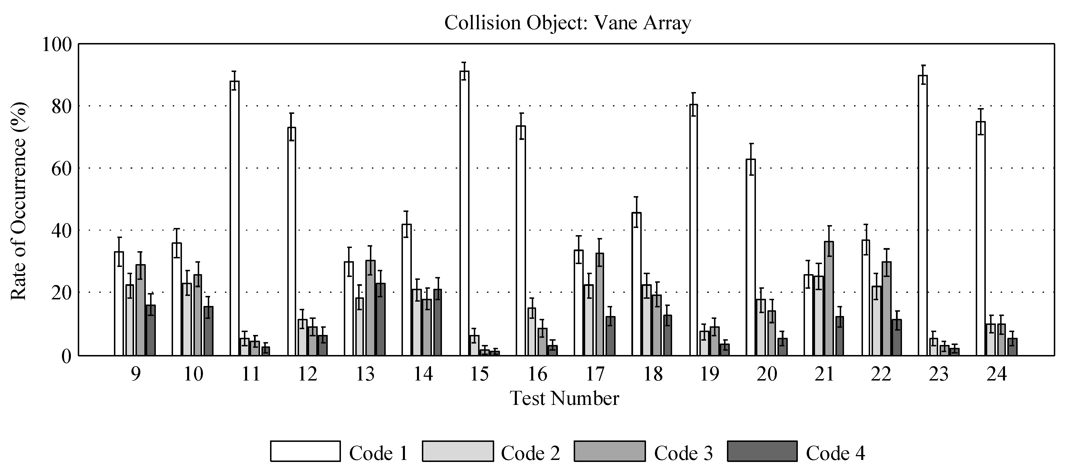
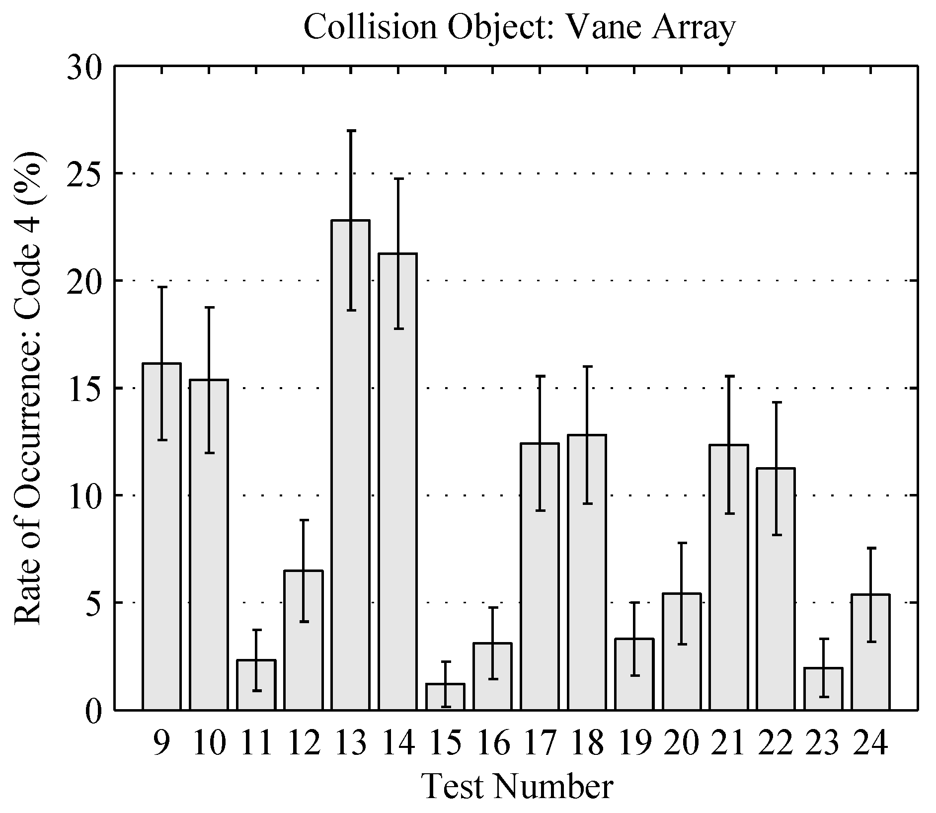
The rates of observed bead passage for each of the four codes defined in Table 2 are presented in Figure 12 for the vane array, and discussed in the following subsections. Please note that all bead collisions occurred on the central stay vane and wicket gate only, and that all beads passed within the range of mm. The collision rates (Code 4) for the vane array geometry are presented in Figure 13 as a subset of the data presented in Figure 12 and will be referenced throughout this section of the article.
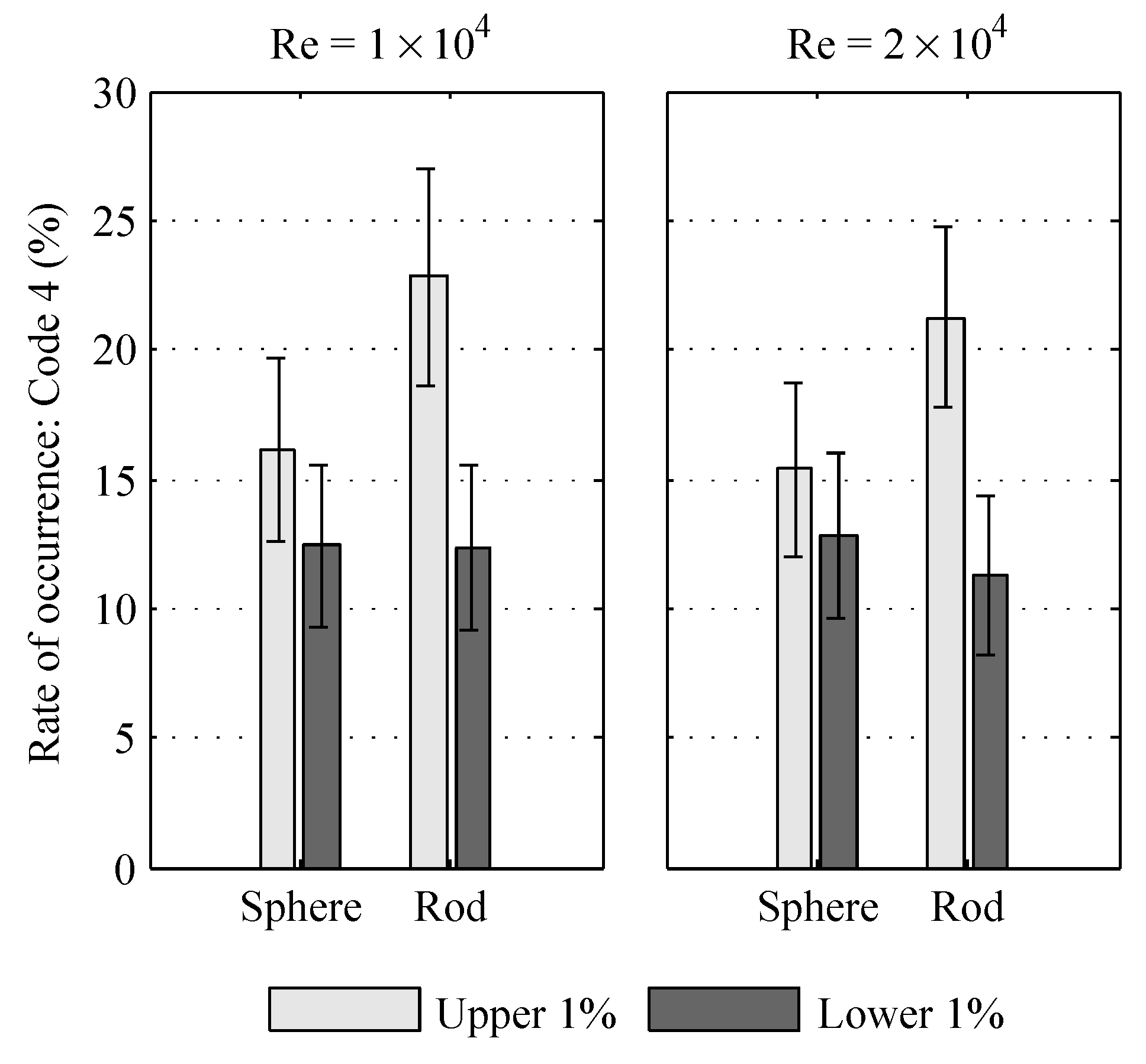
- Wicket Gate Angle:Tests [9–16] vs. [17–24]Increasing the wicket gate angle from the upper 1% angle to the lower 1% setting caused an increase in collision rates, with varying degrees of statistical significance. The experiments with an injection location of are of particular interest in observing this effect (Tests 9–10, 13–14, 17–18, 21–22) as these had notably greater collision rates, for the same reasons as discussed above for the cylinder collision target object. The collision rates of these experiments are plotted in Figure 14.In all cases tested, the collision rates at the upper 1% angle exceeded those at the lower 1% angle. This observation can be interpreted by considering the difference in incident particle distribution between the two cases. The lower 1% wicket gate angle is less aligned with the stay vane than the upper 1% angle, and therefore generates a greater curvature of the streamlines through the vane array than the more streamlined upper 1% configuration. This causes the mean lateral location of the incident bead distribution to be offset by mm. This shift in the lateral distribution is shown graphically in Figure 9 by the white vertical line being offset in the direction for the lower 1% configurations (Tests 17, 18, 21, and 22). The resulting collision rates for both the stay vane and wicket gate are reduced as the bulk of the beads pass to the side of the central stay vane and wicket gate.This trend is observed for all cases compared in Figure 14, but is most exaggerated for the rod-shaped beads where a mean reduction in strike rate of up to 10% was observed as result of the wicket gate angle adjustment. This corresponds to the pairs of experiments with the greatest difference in mean lateral distribution y-ordinates; namely, Test 21 relative to Test 13 and Test 22 relative to Test 14 (see Figure 9).
- Bead Shape:Tests [9–12] vs. [13–16], [17–20] vs. [21–24]No difference in collision rates as a function of bead shape is observed outside of the error ranges calculated. However, for beads released at as shown in Figure 14, the mean collision rates for the spherical beads are approximately 7% less than the collision rates for the rod-shaped beads when the wicket gate angle is set at the upper 1% position (Tests 9–10 vs. 13–14).
- Release Offset:Tests [9–10] vs. [11–12], [13–14] vs. [15–16], [17–18] vs. [19–20], [21–22] vs. [23–24]As with the cylinder tests, a significant decrease in collision rates was observed when release location was offset to . There is a corresponding increase in particle passage with no deviation (Code 1). Again, this is expected as the mean of the lateral bead distribution is offset from the central stay vane to the middle of the gap between stay vane pairs.
- Flow Speed:Tests 9 vs. 10, 11 vs. 12, 13 vs. 14, 15 vs. 16, 17 vs. 18, 19 vs. 20, 21 vs. 22, 23 vs. 24As with the cylinder tests, the flow speed effects showed consistent trends in collision rates, though these were not significant within the error margins of the present experiment. However, the observed trends of flow speed on mean collision rates is best understood by recalling the increased dispersion of the beads at the higher flow speeds. In general, for the beads released at , the increased dispersion causes a reduction in collisions as the spread of the beads away from the central vane reduces the likelihood of collision (Tests 9 vs. 10, 13 vs. 14, 21 vs. 22). The single exception to this observation is the case of the spherical beads at the lower 1% vane angle (Test 17 vs Test 18). For those released at , the increased dispersion accounts for the slight trend of increased collision rate as more beads traverse the lateral offset to the collision object (Tests 11 vs. 12, 15 vs. 16, 19 vs. 20, 23 vs. 24).
4. Discussion
The experimental approach of a point release is a convenient way to introduce the beads into the flow in a way that can be well defined and readily recreated in a computational simulation. The resulting distributions of beads as they approach the collision targets is therefore a result of this bead injection method and is not representative of the true distribution of fish in a hydroturbine intake.
In these experiments, the nature of the incident bead distribution at a given stream-wise location is driven by the flow conditions which were characterized and presented as part of this work. It is, therefore, expected that similar incident bead distributions will be obtained by simulations of this setup when the flow conditions specified in Table 3 are used as inputs. The incident distribution of beads in CFD simulations of these experiments should be similar before any correspondence in collision rates between can be expected. The data set presented herein can be used to validate bead collision simulations or collision detection algorithms by introducing the beads with the measured distributions presented in Figure 9.
The vertical velocity profile was measured to be effectively constant within the vertical range that the beads arrive at the collision targets. Because the collision geometry was constant in the z-direction, the elevation of the beads was not considered in the analysis presented herein.
The results of the current study did not indicate a difference in bead collision rates for the two bead shapes considered outside of the calculated 95% confidence interval (Figure 14). The spherical- and rod-shaped bead collision rates observed during the lower 1% vane configuration tests were particularly similar. In interpreting this result is important to consider that the flow speed and turbulence levels of the experimental facility were not able to match the scaled representative velocity at the distributor. While the flow conditions presented herein therefore do not represent those of the full-scale intake, the data set presented for the conditions defined present a useful and unique resource for the validation of computational models of the equivalent scenario. These validations will be strengthened by future experimental efforts with access to increased velocity and turbulence levels.
The location and intensity of each observed collision were also recorded as part of this experimental campaign. However, the uncertainty of the rates of these observations is significant because the sample size used in Equation (2) is the number of collisions observed which is a subset of the total number of beads. As such, a greater number of bead releases is required to observe a satisfactory number of collisions to achieve a meaningful 95% confidence interval. In tests where the collision rate were < of the total number of beads released, this would require at least an order of magnitude increase in the number of beads released.
The primary application of the data presented herein is to provide validation for computational models using particles to represent fish passing through turbines. This is an important step in building confidence in the results from computational simulation methods for spherical particle trajectories [23] and non-spherical particle trajectories [33]. The acceptance of these new computationally based design methods are expected to have important applications for the turbine manufacturing industry as well as for the environmental regulatory entities.
5. Conclusions
An experimental data set has been collected to advance and validate simulations of fish passage through hydroturbines. These experiments characterized the beads passage of at beads for each of 24 test configurations, where the effect of bead shape, collision object, wicket gate angle, flow speed, and release offset were explored. The flow conditions were measured using an ADV and the resulting incident bead dispersion were measured using particle tracking software. Collision objects and inertial particles were designed to represent relevant hydroturbine geometries using Froude scaling. The observation of the bead trajectories and collisions represent a unique and valuable data set for validating CFD simulations used to predict the biological impact of hydroturbines on fish passage.
Collision rates from 1–7% were observed for the cylinder geometry and rates of 1–23% were observed for the vane array over the range of test configurations. Increasing the wicket gate angle introduced an offset in the distribution mean of the incident particles, causing a reduction in observed collisions for beads released with zero lateral offset. The increased dispersion of the beads with flow speed explained the decrease in collision rates for beads released with zero offset, and increased collision rates for those released at a lateral offset. No bead shape dependencies were observed within the 95% confidence intervals for the experimental flow conditions described.
Though the collision intensity and location were recorded, the relatively low number of collisions events observed resulted in large confidence interval for the rates of occurrence. To quantify the distribution of collision locations and intensities with a 95% confidence in observed rates, the authors suggest increasing the number of beads released to achieve a total number of strike observation of for each test.
Author Contributions
Funding acquisition, M.C.R.; conceptualization, M.C.R. and S.F.H.; methodology, M.C.R., S.F.H. and R.P.M.; investigation, S.F.H. and R.P.M.; writing—original draft, S.F.H.; writing—review and editing, M.C.R., S.F.H. and R.P.M.
Funding
This research was conducted under the Laboratory Directed Research and Development Program at Pacific Northwest National Laboratory, a multi-program national laboratory operated by Battelle for the U.S. Department of Energy.
Acknowledgments
The authors wish to thank Pedro Romero-Gomez for providing CFD solutions to Ice Harbor Dam inlet flow conditions, Ryan Harnish for assistance in the error analysis of the observed bead passage rates, and Jason Serkowski for assistance in video analysis. The authors also wish to thank Natalia Kaiser and the Department of Civil and Environmental Engineering at Washington State University for access and support in the use the test flume.
Conflicts of Interest
The authors declare no conflict of interest.
Appendix A. ADV Velocity Processing
Appendix A.1. Correlation and SNR Filtering
All velocity data with a correlation of less than 70% and signal-to-noise ratio (SNR) of less than 20 dB was not considered in this analysis [34].
Appendix A.2. Phase-Space Filtering
One of the most efficient algorithms for the removal of spikes in a velocity time series measured using an acoustic Doppler device is the ‘phase-space’ method. Originally developed by [35], a revised version of the method identified spurious data points as those which fall outside an ellipsoidal envelope of acceptance when each velocity data point is plotted against its derivatives [36]. As the magnitude of the ellipsoidal threshold is a function of the standard deviation of the data and its derivatives, the process is iterated until all the points are located within the ellipsoidal volume. To maintain a continuous data set after this filtering method has been applied, rejected data points are replaced using a cubic interpolation of accepted velocity points. This algorithm was implemented using the despiking functions developed as part of the MACE Toolbox for MATLAB [37].
Appendix A.3. Doppler Noise Removal
Doppler noise is a characteristic of ADV velocity measurement and is manifested as white noise in the velocity spectra [38]. The receiver geometry of the Nortek Vectrino allows for the direction in line with the transducer axis to be resolved with a lower noise floor than the transverse plane [28]. The standard velocity (RMS) error introduced by Doppler noise for each velocity direction (, and ) was identified from the energy spectra of each velocity component, and removed from the standard deviation of the velocity signal (, and ) [39,40]. This process is shown for the case of the u direction in Equation (A1), where . The RMS velocity corrected for the Doppler noise contribution is denoted with an asterisk.
The turbulent kinetic energy, k, describes the total turbulent energy production and is calculated as a function of the noise-corrected velocity standard deviations as shown by Equation (A2).
The turbulence velocity metric, , which represents the characteristic three-dimensional RMS velocity, is then calculated as . The turbulence intensity is commonly presented as a metric of turbulence velocity relative to the mean flow velocity and is calculated as .
Though the noise floor of the ADV measurement can be accounted for by subtracting the noise energy from the measured turbulent energy in the calculation of the bulk statistics of k, and , the high contribution of Doppler noise at the higher frequencies reduces the accuracy of the calculation of higher moment flow metrics [39]. However, the low magnitude of observed turbulence fluctuations indicates that these metrics will have a limited influence on the bead observations, which constitute the focus of this paper. For these reasons, further flow analysis and metrics are not presented.
References
- Coutant, C.C.; Whitney, R.R. Fish behavior in relation to passage through hydropower turbines: A review. Trans. Am. Fish. Soc. 2000, 129, 351–380. [Google Scholar] [CrossRef]
- Schilt, C.R. Developing fish passage and protection at hydropower dams. Appl. Anim. Behav. Sci. 2007, 104, 295–325. [Google Scholar] [CrossRef]
- Cada, G.F. The development of advanced hydroelectric turbines to improve fish passage survival. Fisheries 2001, 26, 14–23. [Google Scholar] [CrossRef]
- Dauble, D.D.; Deng, Z.D.; Richmond, M.C.; Moursund, R.; Carlson, T.J.; Rakowski, C.L.; Duncan, J. Biological Assessment of the Advanced Turbine Design at Wanapum Dam, 2005; Technical Report; PNNL-16682; Pacific Northwest National Laboratory: Richland, WA, USA, 2007. [CrossRef]
- Dedual, M. Survival of juvenile rainbow trout passing through a Francis turbine. N. Am. J. Fish. Manag. 2007, 27, 181–186. [Google Scholar] [CrossRef]
- Mathur, D.; Heisey, P.; Skalski, J.; Kenney, D.R. Salmonid smolt survival relative to turbine efficiency and entrainment depth in hydroelectric power generation. J. Am. Water Resour. Assoc. 2000, 36, 737–747. [Google Scholar] [CrossRef]
- Deng, Z.; Carlson, T.J.; Duncan, J.P.; Richmond, M.C. Six-Degree-of-Freedom Sensor Fish Design and Instrumentation. Sensors 2007, 7, 3399–3415. [Google Scholar] [CrossRef] [PubMed] [Green Version]
- Fu, T.; Deng, Z.D.; Duncan, J.P.; Zhou, D.; Carlson, T.J.; Johnson, G.E.; Hou, H. Assessing hydraulic conditions through Francis turbines using an autonomous sensor device. Renew. Energy 2016, 99, 1244–1252. [Google Scholar] [CrossRef] [Green Version]
- Richmond, M.C.; Serkowski, J.A.; Ebner, L.L.; Sick, M.; Brown, R.S.; Carlson, T.J. Quantifying barotrauma risk to juvenile fish during hydro-turbine passage. Fish. Res. 2014, 154, 152–164. [Google Scholar] [CrossRef] [Green Version]
- Richmond, M.C.; Serkowski, J.A.; Rakowski, C.; Strickler, B.; Weisbeck, M. Computational tools to assess turbine biological performance. Hydro Rev. 2014, 33, 88–98. [Google Scholar]
- Richmond, M.C.; Romero-Gomez, P.; Serkowski, J.A.; Rakowski, C.L.; Graf, M.J. Comparative Study of Barotrauma Risk During Fish Passage Through Kaplan Turbines; PNNL-SA-113640; Technical Report; Pacific Northwest National Laboratory: Richland, WA, USA, 2015. [CrossRef]
- Qureshi, N.M.; Bourgoin, M.; Baudet, C.; Cartellier, A.; Gagne, Y. Turbulent transport of material particles: An experimental study of finite size effects. Phys. Rev. Lett. 2007, 99, 1–4. [Google Scholar] [CrossRef] [PubMed]
- Qureshi, N.M.; Arrieta, U.; Baudet, C.; Cartellier, A.; Gagne, Y.; Bourgoin, M. Acceleration statistics of inertial particles in turbulent flow. Eur. Phys. J. B 2008, 66, 531–536. [Google Scholar] [CrossRef] [Green Version]
- Xu, H.; Bodenschatz, E. Motion of inertial particles with size larger than Kolmogorov scale in turbulent flows. Phys. D Nonlinear Phenom. 2008, 237, 2095–2100. [Google Scholar] [CrossRef]
- Bagheri, G.H.; Bonadonna, C.; Manzella, I.; Pontelandolfo, P.; Haas, P. Dedicated vertical wind tunnel for the study of sedimentation of non-spherical particles. Rev. Sci. Instrum. 2013, 84. [Google Scholar] [CrossRef] [PubMed]
- Ren, B.; Zhong, W.; Jin, B.; Lu, Y.; Chen, X.; Xiao, R. Study on the drag of a cylinder-shaped particle in steady upward gas flow. Ind. Eng. Chem. Res. 2011, 50, 7593–7600. [Google Scholar] [CrossRef]
- Horowitz, M.; Williamson, C.H.K. The effect of Reynolds number on the dynamics and wakes of freely rising and falling spheres. J. Fluid Mech. 2010, 651, 251–294. [Google Scholar] [CrossRef]
- Machicoane, N.; Zimmermann, R.; Fiabane, L.; Bourgoin, M.; Pinton, J.F.; Volk, R. Large sphere motion in a nonhomogeneous turbulent flow. New J. Phys. 2014, 16. [Google Scholar] [CrossRef]
- Zenit, R.; Hunt, M.L. Mechanics of immersed particle collisions. J. Fluids Eng. Trans. ASME 1999, 121, 179–184. [Google Scholar] [CrossRef]
- Joseph, G.G.; Zenit, R.; Hunt, M.L.; Rosenwinkel, A.M. Particle–wall collisions in a viscous fluid. J. Fluid Mech. 2001, 433, 329–346. [Google Scholar] [CrossRef] [Green Version]
- Conger, R.; Ramaprian, B.R. Pressure measurements on a pitching airfoil in a water channel. AIAA J. 1994, 32, 108–115. [Google Scholar] [CrossRef]
- Oshima, H.; Ramaprian, B.R. Velocity Measurements over a Pitching Airfoil. AIAA J. 1997, 35, 119–126. [Google Scholar] [CrossRef]
- Romero-Gomez, P.; Richmond, M.C. Movement and collision of Lagrangian particles in hydro-turbine intakes: A case study. J. Hydraul. Res. 2017, 55, 706–720. [Google Scholar] [CrossRef]
- Kenney, J.F.; Keeping, E.S. Mathematics of Statistics, 3rd ed.; Van Nostrand: Princeton, NJ, USA, 1962; Volume 1. [Google Scholar]
- Deng, Z.D.; Lu, J.; Myjak, M.J.; Martinez, J.J.; Tian, C.; Morris, S.J.; Carlson, T.J.; Zhou, D.; Hou, H. Design and implementation of a new autonomous sensor fish to support advanced hydropower development. Rev. Sci. Instrum. 2014, 85. [Google Scholar] [CrossRef] [PubMed]
- Nortek AS. Vectrino Data Sheet; Nortek AS: Rud, Norway, 2017; Available online: www.nortekusa.com/lib/data-sheets/datasheet-vectrino-lab (accessed on 14 January 2019).
- Rusello, P. A Practical Primer for Pulse Coherent Instruments; Technical Report, Nortek Technical Note No.: TN-027; Nortek: Bologna, Italy, 2009. [Google Scholar]
- Hurther, D.; Lemmin, U. A correction method for turbulence measurements with a 3D acoustic doppler velocity profiler. J. Atmos. Ocean. Technol. 2001, 18, 446–458. [Google Scholar] [CrossRef]
- Nortek AS. Comprehensive Manual; Technical Report; Nortek AS: Bologna, Italy, 2015. [Google Scholar]
- Photron Ltd. FASTCAM Mini UX50/100 Hardware Manual; Photron Ltd.: Tokyo, Japan, 2014. [Google Scholar]
- Hulley, S.; Cummings, S.; Browner, W.; Grady, D.; Newman, T. Designing Clinical Research: An Epidemiological Approach, 4th ed.; Lippincott Williams & Wilkins: Philadelphia, PA, USA, 2013. [Google Scholar]
- Xcitex Inc. ProAnalyst Motion Analysis Software User Guide; Xcitex Inc.: Woburn, MA, USA, 2017. [Google Scholar]
- Richmond, M.C.; Romero-Gomez, P. Fish passage through hydropower turbines: Simulating blade strike using the discrete element method. IOP Conf. Ser. Earth Environ. Sci. 2014, 22, 1–10. [Google Scholar] [CrossRef]
- Rusello, P.; Lohrmann, A.; Siegel, E.; Maddux, T. Improvements in acoustic Doppler velocimetery. In Proceedings of the 7th International Conference in Hydroscience and Engineering (ICHE 2006), Philadelphia, PA, USA, 10–13 September 2006. [Google Scholar]
- Goring, D.G.; Nikora, V.I. Despiking acoustic Doppler velocimeter data. J. Hydraul. Eng. 2002, 128, 117–126. [Google Scholar] [CrossRef]
- Mori, N.; Suzuki, T.; Kakuno, S. Noise of acoustic Doppler velocimeter data in bubbly flow. ASCE J. Eng. Mech. 2007, 133, 122–125. [Google Scholar] [CrossRef]
- Mori, N. MACE Toolbox. 2009. Available online: http://www.oceanwave.jp/softwares/mace/index.php?MACE%20Softwares (accessed on 14 January 2019).
- Durgesh, V.; Thomson, J.; Richmond, M.C.; Polagye, B.L. Noise correction of turbulent spectra obtained from acoustic doppler velocimeters. Flow Meas. Instrum. 2014, 37, 29–41. [Google Scholar] [CrossRef]
- García, C.M.; Cantero, M.I.; Niño, Y.; García, M.H. Turbulence Measurements with Acoustic Doppler Velocimeters. J. Hydraul. Eng. 2005, 131, 1062–1073. [Google Scholar] [CrossRef]
- Thomson, J.; Polagye, B.; Richmond, M.; Durgesh, V. Quantifying turbulence for tidal power applications. In Proceedings of the OCEANS 2010 MTS/IEEE SEATTLE, Seattle, WA, USA, 20–23 September 2010. [Google Scholar]
Figure 1.
Computational model of Ice Harbor Dam [23] showing representative horizontal flow velocity in the intake and distributor. The horizontal direction is defined as being perpendicular to runner axis.
Figure 1.
Computational model of Ice Harbor Dam [23] showing representative horizontal flow velocity in the intake and distributor. The horizontal direction is defined as being perpendicular to runner axis.

Figure 2.
Schematic of test section of recirculating water flume showing bead injector tube and vane array installation.
Figure 2.
Schematic of test section of recirculating water flume showing bead injector tube and vane array installation.

Figure 3.
Collision geometry: (a) cylinder and (b) stay vane and wicket gate array. The details of the stay vane and wicket gate configuration is shown in (c).
Figure 3.
Collision geometry: (a) cylinder and (b) stay vane and wicket gate array. The details of the stay vane and wicket gate configuration is shown in (c).

Figure 4.
Spherical and cylindrical bead design.

Figure 5.
Dual high-speed cameras show spherical bead passage through vane array at upper 1% configuration (Test 5).
Figure 5.
Dual high-speed cameras show spherical bead passage through vane array at upper 1% configuration (Test 5).

Figure 6.
Experimental photographs of bead injection and passage. (a) Injection tube showing the release of rod-shaped beads into flume; (b) Bead passage through vane array, viewed from the downstream end of the flume (in -x direction).
Figure 6.
Experimental photographs of bead injection and passage. (a) Injection tube showing the release of rod-shaped beads into flume; (b) Bead passage through vane array, viewed from the downstream end of the flume (in -x direction).

Figure 7.
Transverse velocity profiles of mean flow velocity for the (a) cylinder and (b) vane array collision geometries at . The velocity profiles were measured at mid-depth () across four stream-wise locations in the flume; one upstream of the collision geometry (), and three downstream ().
Figure 7.
Transverse velocity profiles of mean flow velocity for the (a) cylinder and (b) vane array collision geometries at . The velocity profiles were measured at mid-depth () across four stream-wise locations in the flume; one upstream of the collision geometry (), and three downstream ().

Figure 8.
Histograms showing vertical distributions of beads at for selected tests. The distribution mean is shown with a light grey line for each test. The extent of the y-axis of these plots is equal to the length of the collision objects.
Figure 8.
Histograms showing vertical distributions of beads at for selected tests. The distribution mean is shown with a light grey line for each test. The extent of the y-axis of these plots is equal to the length of the collision objects.

Figure 9.
Histograms showing lateral distributions of beads at for tests with lateral release location of . The distribution mean is shown with a vertical grey line for each test.
Figure 9.
Histograms showing lateral distributions of beads at for tests with lateral release location of . The distribution mean is shown with a vertical grey line for each test.

Figure 10.
Summary of bead passage codes for cylinder tests, showing 95% confidence interval of observed rates.
Figure 10.
Summary of bead passage codes for cylinder tests, showing 95% confidence interval of observed rates.

Figure 11.
Collision rate (Code 4) with cylinder.

Figure 12.
Summary of bead passage codes for vane array tests, showing 95% confidence interval of observed rates.
Figure 12.
Summary of bead passage codes for vane array tests, showing 95% confidence interval of observed rates.

Figure 13.
Collision rate (Code 4) with vane array.

Figure 14.
Influence of wicket gate angle on bead passage.


Table 1.
Experimental test matrix.
| Test # | Target Shape | Wicket Gate Angle | Bead Shape | Release Offset (Δ) | () |
|---|---|---|---|---|---|
| 1 | Cylinder | N/A | Sphere | 0 | |
| 2 | Cylinder | N/A | Sphere | 0 | |
| 3 | Cylinder | N/A | Sphere | ||
| 4 | Cylinder | N/A | Sphere | ||
| 5 | Cylinder | N/A | Rod | 0 | |
| 6 | Cylinder | N/A | Rod | 0 | |
| 7 | Cylinder | N/A | Rod | ||
| 8 | Cylinder | N/A | Rod | ||
| 9 | Vane Array | Upper 1% | Sphere | 0 | |
| 10 | Vane Array | Upper 1% | Sphere | 0 | |
| 11 | Vane Array | Upper 1% | Sphere | ||
| 12 | Vane Array | Upper 1% | Sphere | ||
| 13 | Vane Array | Upper 1% | Rod | 0 | |
| 14 | Vane Array | Upper 1% | Rod | 0 | |
| 15 | Vane Array | Upper 1% | Rod | ||
| 16 | Vane Array | Upper 1% | Rod | ||
| 17 | Vane Array | Lower 1% | Sphere | 0 | |
| 18 | Vane Array | Lower 1% | Sphere | 0 | |
| 19 | Vane Array | Lower 1% | Sphere | ||
| 20 | Vane Array | Lower 1% | Sphere | ||
| 21 | Vane Array | Lower 1% | Rod | 0 | |
| 22 | Vane Array | Lower 1% | Rod | 0 | |
| 23 | Vane Array | Lower 1% | Rod | ||
| 24 | Vane Array | Lower 1% | Rod |
Table 2.
Bead passage codes.
| Code | Description |
|---|---|
| 1 | Minimal deviation in trajectory |
| 2 | Moderate deviation in trajectory |
| 3 | Significant deviation in trajectory |
| 4 | Collision |
Table 3.
Incident flow velocity metrics.
| U (m/s) | 0.26 | 0.53 |
| V (m/s) | 0.00 | 0.00 |
| W (m/s) | 0.00 | 0.00 |
| (mm/s) | 1.4 | 1.5 |
| (mm/s) | 1.7 | 2.7 |
| (mm/s) | 1.4 | 2.3 |
| k | 3.4 | 7.3 |
| (mm/s) | 1.5 | 2.2 |
| (%) | 0.58 | 0.42 |
© 2019 by the authors. Licensee MDPI, Basel, Switzerland. This article is an open access article distributed under the terms and conditions of the Creative Commons Attribution (CC BY) license (http://creativecommons.org/licenses/by/4.0/).
Share and Cite
MDPI and ACS Style
Harding, S.F.; Richmond, M.C.; Mueller, R.P. Experimental Observation of Inertial Particles through Idealized Hydroturbine Distributor Geometry. Water 2019, 11, 471. https://doi.org/10.3390/w11030471
AMA Style
Harding SF, Richmond MC, Mueller RP. Experimental Observation of Inertial Particles through Idealized Hydroturbine Distributor Geometry. Water. 2019; 11(3):471. https://doi.org/10.3390/w11030471
Chicago/Turabian StyleHarding, Samuel F., Marshall C. Richmond, and Robert P. Mueller. 2019. "Experimental Observation of Inertial Particles through Idealized Hydroturbine Distributor Geometry" Water 11, no. 3: 471. https://doi.org/10.3390/w11030471
Note that from the first issue of 2016, this journal uses article numbers instead of page numbers. See further details here.