Investigation of Free Surface Turbulence Damping in RANS Simulations for Complex Free Surface Flows


1
Department of Civil and Environmental Engineering, Norwegian University of Science of Technology, NTNU, 7491 Trondheim, Norway
2
Department of Hydraulic and Water Resources Engineering, Budapest University of Technology and Economics, Moegyetem rkp. 3, 1111 Budapest, Hungary
*
Author to whom correspondence should be addressed.
Water 2019, 11(3), 456; https://doi.org/10.3390/w11030456
Submission received: 1 February 2019
/
Revised: 21 February 2019
/
Accepted: 25 February 2019
/
Published: 4 March 2019
(This article belongs to the Special Issue Advances in Hydraulics and Hydroinformatics)
Abstract
:The modelling of complex free surface flows over weirs and in the vicinity of bridge piers is presented in a numerical model emulating open channel flow based on the Reynolds Averaged Navier-Stokes (RANS) equations. The importance of handling the turbulence at the free surface in the case of different flow regimes using an immiscible two-phase RANS Computational Fluid Dynamics (CFD) model is demonstrated. The free surface restricts the length scales of turbulence and this is generally not accounted for in standard two-equation turbulence modelling approaches. With the two-phase flow approach, large-velocity gradients across the free surface due to the large difference in the density of the fluids can lead to over-production of turbulence. In this paper, turbulence at the free surface is restricted with an additional boundary condition for the turbulent dissipation. The resulting difference in the free surface features and the consequences for the solution of the flow problem is discussed for different flow conditions. The numerical results for the free surface and stream-wise velocity gradients are compared to experimental data to show that turbulence damping at the free surface provides a better representation of the flow features in all the flow regimes and especially in cases with rapidly varying flow conditions.
1. Introduction
The interface between air and water or the free water surface is one of the most significant features of open channel flow. The motion of the free surface and the flow properties such as velocities and the pressure in the flow are strongly related. A change in the geometry of the channel, such as in the case of flow around hydraulic structures, steep pressure gradients occur due to flow constriction. According to Bernoulli’s equation, under ideal conditions the total energy in the flow is conserved through transfer of energy between potential and kinetic energy. In addition, energy is lost to fluid-fluid and fluid-solid interface friction. This results in a change in the free surface location and the flow features, and governs the design of hydraulic structures.
The free surface features resulting from different flow conditions such as hydraulic jumps, shock waves, and standing waves can have negative consequences on the hydraulic structure and should be considered during design. Several researchers have proposed different empirical formulae to estimate different features such as the height of a shock front or deflection angles [1,2,3,4]. Physical model tests investigating different flow conditions and the resulting flow features can provide more details regarding the flow phenomena [5,6,7,8].
Numerical modelling of the open channel flow phenomena can yield further detail into the flow physics. Due to the strong relationship between the flow hydrodynamics and the free surface, the correct representation of the free surface along with the boundary conditions are essential to accurately represent the flow in a numerical model. Over recent decades many different methods for the prediction of the free water surface elevation have been developed. They reach from simple empirical estimations with 1D numerical tools, e.g., Brunner [9] to more advanced 3D models, e.g., Olsen [10].
The application of Computational Fluid Dynamics (CFD) methods to study free surface flows is an interesting avenue where different flow features can be calculated in detail with the solution of the Navier-Stokes equations, where the Reynolds Averaged Navier-Stokes (RANS) framework is employed [11,12]. Further several recent studies in literature present eddy-resolving frameworks such as Kirkil et al. [13], Kara et al. [14], Kang and Sotiropoulos [15] and McSherry et al. [16]. Eddy-resolving simulations provide a higher level of detail regarding the coherent structures in a turbulent flow and a better resolution of the flow compared to the RANS models [17]. On the other hand, the potential of the RANS models to evaluate complex free surface flows without resolving details regarding the turbulent eddies is not yet fully used. Unsteady RANS simulations offer a balance between computational efficiency and resolution of the flow, which can be used for many engineering applications. A challenge with two-phase RANS simulations is that the effect of the free surface is not accounted for in the standard RANS turbulence models. The turbulence production is determined by the strain rate in fluids and at the interface, the abrupt large difference in the fluid density leads to a high turbulence production. In reality, the presence of the free surface results in the elongation of the turbulent eddies parallel to the flow and dissipation of the turbulent energy in the direction normal to the free surface. This turbulence dissipation at the free surface must be included using additional boundary conditions in RANS turbulence models.
Several authors have presented different approaches to overcome this limitation in the RANS equations for two-phase flow. Jacobsen et al. [18] proposed an alternative method to calculate the turbulence production in the two-equation turbulence models for two-phase CFD models using the vorticity in the flow instead of the strain rate to avoid the over-production of turbulence around the free surface. Devolder et al. [19] demonstrated excessive damping of the free surface due to the over-production of turbulence around the free surface with the SST model in OpenFOAM and proposed a buoyancy modification term to account for this problem. Furthermore, Larsen and Fuhrman [20] showed that the overestimation of turbulence around the free surface is inherent in the classical RANS turbulence modelling approach and proposed a new closure term to avoid the exponential growth of the eddy viscosity.
In the current study, the relationship shown by Naot and Rodi [21], following the concept of wall function dissipation adjusted to free surface conditions based on experimental observations is implemented to address turbulence over-production around the free surface. This provides a boundary condition for the turbulence dissipation around the free surface based on the flow physics. The boundary condition is implemented in the open-source CFD model, REEF3D [22] and used to study complex flow features downstream of different hydraulic structures for different flow conditions. The model has been previously applied to various problems in which the representation of the complex deformation of the free surface is essential such as wave trapping between cylinders [23], breaking wave forces [24,25], breaking wave kinematics [26] and floating bodies on waves [27].
The influence of the free surface turbulence boundary condition is investigated for various flow cases in this paper to demonstrate the applicability of the method in a universal manner to complex free surface flows. Numerical simulations are carried out for controlled and free stream outflow conditions to obtain different flow conditions such as sub-critical flow throughout the domain, change from sub-critical to super-critical flow regime, transitional flow, and change from sub-critical to super-critical and back to sub-critical. These changing flow conditions are investigated for free surface flow over hydraulic structures such an embankment weir, a broad-crested weir and in the vicinity of bridge piers with focus on the boundary condition for the turbulence dissipation at the free surface. The numerical results for the free surface and the stream-wise velocity profiles over the water depth are compared to experimental data. The change in the distribution of the eddy viscosity around the free surface and the stream-wise velocity profiles in the presence and absence of the free surface turbulence boundary condition is also analyzed to investigate the influence and importance of turbulence damping at the free surface in the different cases.
2. Numerical Model
REEF3D uses the incompressible RANS equations together with the continuity equation to solve the immiscible two-phase fluid flow problem:
where u is the time averaged velocity, is the density of the fluid, p is the pressure, is the kinematic viscosity, is the eddy viscosity and g the acceleration due to gravity. The equations are solved simultaneously for the two phases and the location of the free surface determines the material properties of the fluid cell such as density and viscosity.
The projection method [28] is used for pressure treatment and the resulting Poisson pressure equation is solved with a geometric multigrid preconditioned BiCGStab solver [29] provided by the high-performance solver library, HYPRE [30]. Turbulence modelling is carried out using the two-equation model [31]:
where k is the turbulent kinetic energy, is the specific turbulent dissipation rate, is the turbulent production rate, the coefficients have the values , , , and .
This turbulence model is chosen as it is the most suitable for two-phase flow calculations with unsteady flow situations as in the cases presented in this study. This is because model tends to be numerically more stable due to the linear relationship between k and , . In comparison, the model defines this relationship with a quadratic term as in , which can lead to issues with numerical stability for areas of low levels of turbulence intensity.
To avoid the over-production of eddy viscosity outside the boundary layer in simulations of highly strained flow, eddy-viscosity limiters proposed by [32] are used:
where is the magnitude of the strain tensor.
The free surface influences the turbulence in such a way that the components normal to the surface are damped whereas the components parallel to the surface are enhanced. This is included in the turbulence model through an additional boundary condition at the free surface as shown by [21]. Here, the specific turbulence dissipation term at the free surface is defined as:
where and . The variable is the virtual origin of the turbulent length scale, and was empirically found to be 0.07 times the mean water depth [33]. Including the distance from the nearest wall gives a smooth transition from the free surface value to the wall boundary value of . The damping is carried out only around the interface using the Dirac delta function :
where is the width over which the delta function is applied and dx is the grid size. The value is chosen to ensure that at least one grid cell is included around the interface in each direction and the boundary condition is applied just around the interface.
2.1. Free Surface
The free surface is determined with the level set method. The zero-level set of a signed distance function is used to represent the interface between air and water [34]. Moving away from the interface, the level set function gives the shortest distance from the interface. The sign of the function distinguishes between the two fluids across the interface as shown in Equation (8):
The level set function is moved under the influence of the velocity field obtained from the solution of the RANS equations to represent the change in the free surface as the simulation progresses, with the convection equation in Equation (9):
The kinematic and dynamic boundary conditions at the free surface are implicitly enforced by the level set function. The discontinuity in the material properties such as the density and viscosity are handled using an interpolation with the Heaviside function around the interface over a distance of 2.1 [22]. The level set function loses its signed distance property on convection and is reinitialized after every iteration using a partial differential equation-based reinitialization procedure [35] to regain its signed distance property.
2.2. Discretization Schemes
The fifth-order conservative finite difference Weighted Essentially Non-Oscillatory (WENO) scheme [36] is applied to discretize the convective terms of the RANS equations. The level set function, turbulent kinetic energy and the specific turbulent dissipation rate are discretized using the Hamilton-Jacobi formulation of the WENO scheme [37]. The WENO scheme is a minimum third-order accurate and numerically stable even in the presence of large gradients. Time advancement for the momentum and level set equations is carried out using a Total Variation Diminishing (TVD) third-order Runge-Kutta explicit time scheme [38]. Adaptive time stepping is employed to satisfy the CFL criterion based on the maximum velocity in the domain. This ensures numerical stability throughout the simulation with an optimal value of time step size. An implicit scheme is used for the time advancement of the turbulent kinetic energy and the specific turbulent dissipation, as these variables are mostly source term driven with a low influence of the convective terms. Diffusion terms of the velocities are also subjected to implicit treatment to remove them from the CFL criterion. The numerical model has been validated in detail by Bihs et al. [22] and the convergence and order of the model presented. The model is found to be monotonically convergent with the convergence ratio . The combination of the higher-order schemes results in a combined order of about for the model.
The numerical model uses a Cartesian grid for the spatial discretization together with the Immersed Boundary Method (IBM) to represent the irregular boundaries in the domain. Berthelsen and Faltinsen [39] developed the local directional ghost cell IBM to extend the solution smoothly in the same direction as the discretization, which is adapted to three dimensions in the current model. REEF3D is fully parallelized using the domain decomposition strategy and Message Passing Interface (MPI).
3. Numerical Setup
The free surface flow features in open channel flow vary with the flow conditions. Depending on the boundary conditions, the flow around hydraulic structures can stay sub-critical throughout, change from a sub-critical to a super-critical flow or change from sub-critical to super-critical and then back to a sub-critical flow. An overview of the flow conditions and cases investigated is provided in Table 1. The details regarding numerical setup and boundary conditions are provided in this section.
3.1. General Boundary Conditions
In all the cases presented in this study, a logarithmic velocity profile is prescribed at the inflow for the water phase. The air velocities are not prescribed and are a part of the solution. The outflow boundary condition for the simulations with an embankment weir is a zero-gradient or free stream outflow condition, where no resistance is offered to the flow. The required tailwater level in the different cases is maintained using a rectangular obstacle placed towards the end of the channel to represent the outflow gate in the experiments. The free stream outflow boundary condition is also applied in the simulation of the rectangular weir where the flow transitions from sub-critical to super-critical. In the case of the bridge piers, the tailwater level is prescribed at the outflow. The side walls in the two-dimensional numerical channel are treated with a zero-gradient Neumann condition, whereas a no-slip wall boundary condition is used in the three-dimensional channel. A no-slip wall boundary condition is enforced at the bottom of the channel and a zero-gradient Neumann condition is applied to the top of the numerical channel in all the simulations. An initial water depth is prescribed to initialize the free surface in the channel at and a discharge given in the experiments is also prescribed. A Cartesian grid is employed in all the simulations with for all the cases.
3.2. Sub-Critical Flow
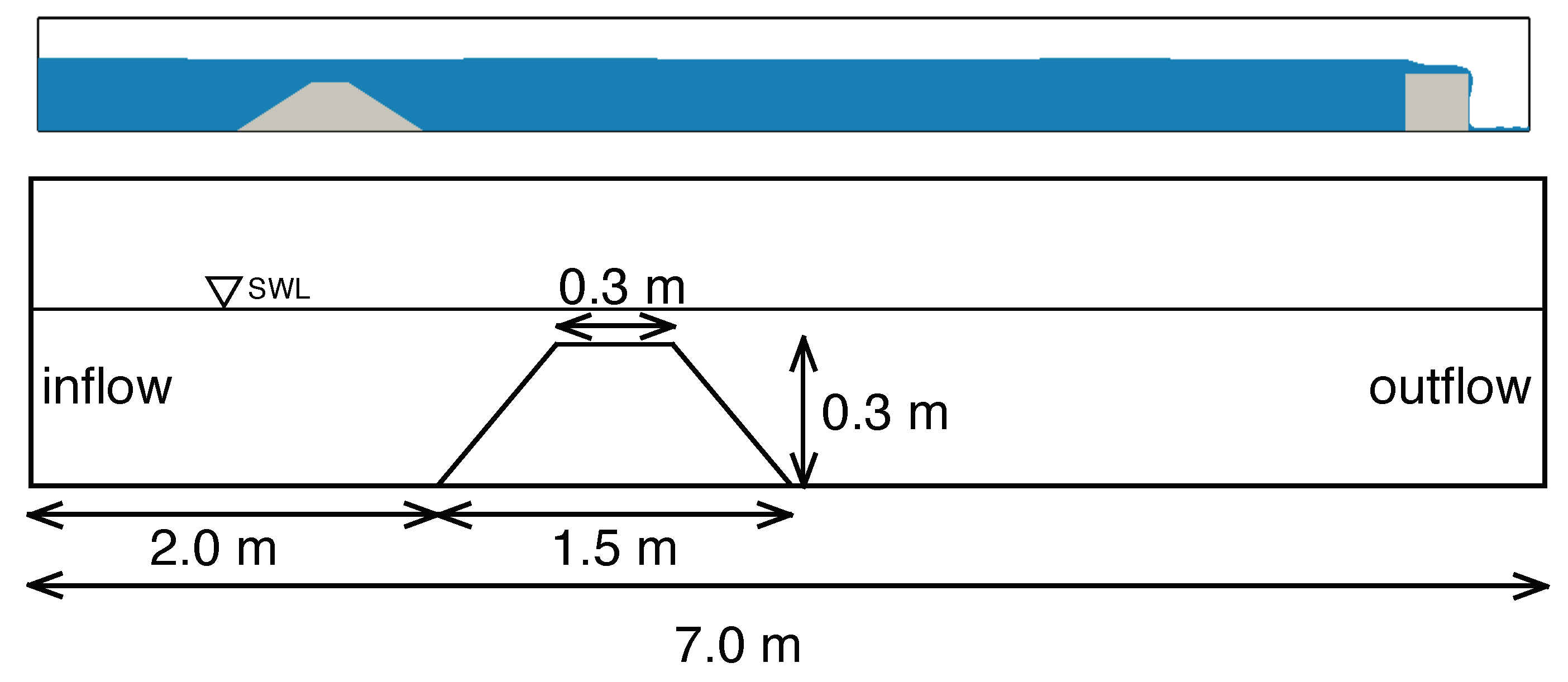
The first case for this flow condition is the experiment carried out for submerged overflow on an embankment weir by Fritz and Hager [5]. The experiments are carried out in a channel 7 m long, m wide and m high. The embankment weir is m high and m long, with a slope of 1VH on both the upstream and downstream faces. The two-dimensional numerical channel setup is similar to the experimental setup and is illustrated in Figure 1 showing the water and air phases within the outline of the channel. The channel has a length of 12 m and a height of m, and the water depth is initialized as m and a discharge of /s/m is specified. The tailwater level in the channel is maintained at m using a rectangular obstacle of height m and length m placed at m in the channel. Stream-wise velocity profiles are calculated at four locations in the channel, upstream of the weir at m, on the upstream face at m, over the downstream toe at m and downstream of the weir at m.
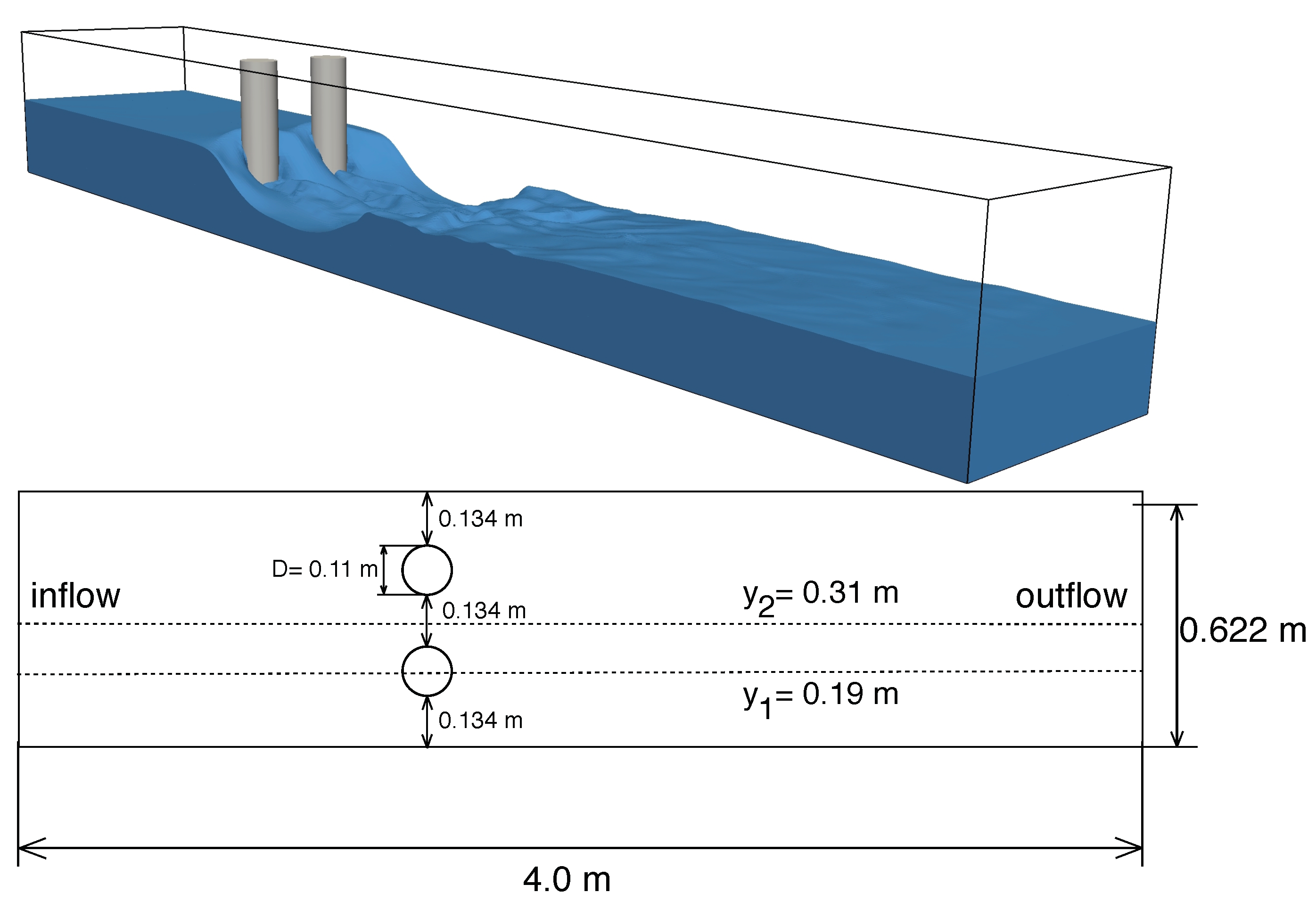
The second case for this flow condition is the flow around a pair of bridge piers presented by Szydłowski [40]. The channel in the experiments is 15 m long, m wide and a pair of bridge piers of diameter m are placed 2 m downstream of the inflow section equidistant from each other and the channel walls. The numerical setup is m long, m wide and m high. The water depth is initialized to m at s and the tailwater level is prescribed to be m along with a discharge of m/s in the channel. The piers are placed m from the inflow region, equidistant from the channel walls and from each other with a distance of m. Stream-wise velocity profiles are calculated at four locations, upstream of the piers at m, in between the piers at m, downstream of the piers at m and m. The numerical setup is illustrated in Figure 2 showing the water and air phases within the outline of the numerical channel and the piers.
3.3. Sub-Critical to Super-Critical Flow
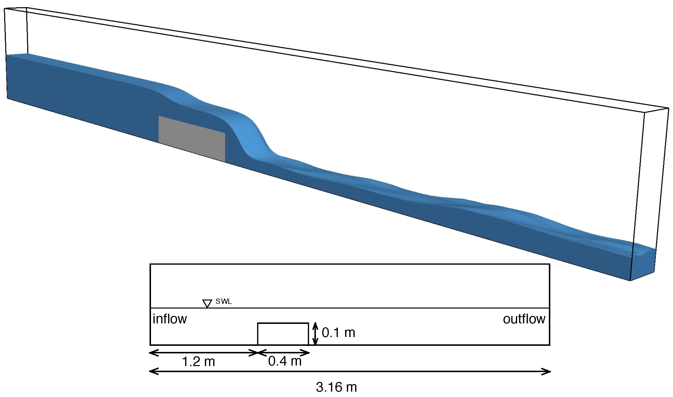
The experiment presented by Sarker and Rhodes [41] for flow over a rectangular broad-crested weir is simulated for this flow condition. The experimental channel is m long and m wide. A rectangular weir with sharp edges m long and m high is placed in the channel with a discharge of /s. The numerical setup is illustrated in Figure 3 showing the outline of the numerical channel, the water, and air phases and the weir. The numerical domain is m long, m wide and m high. The broad-crested weir is m long and m high as in the experiments and placed at m from the inlet. The free surface elevation at the inflow and the discharge are prescribed to be m and /s respectively, using the values from the experimental data.
3.4. Transitional Flow
For this flow condition, the plunging jet flow resulting from a submergence of the embankment weir presented by Fritz and Hager [5] is presented. The numerical setup is similar to that illustrated in Figure 1, with the height of the rectangular obstacle set to m to maintain a tailwater level of m. A discharge of /s/m is specified in the two-dimensional channel. The water depth is initialized at m at s in the simulation. Stream-wise velocity profiles are calculated at four locations in the channel, upstream of the weir at m, on the upstream face at m, over the downstream toe at m and downstream of the weir at m.
3.5. Sub-Critical to Super-Critical to Sub-Critical Flow
The first case for this flow condition is the free overflow on an embankment weir presented by Fritz and Hager [5]. The two-dimensional numerical channel is the same as that illustrated in Figure 1. The tailwater level is maintained at m using a rectangular obstacle of height m. A discharge of /s/m is prescribed in the two-dimensional channel and the water depth is initialized at m at s. Stream-wise velocity profiles are calculated at four locations in the channel, upstream of the weir at m, on the upstream face at m, over the downstream toe at m and downstream of the weir at m.
The second case for this flow condition is the flow around a pair of bridge piers presented by Szydłowski [40], using the numerical setup illustrated in Figure 2, but with a height of m. A tailwater level of m, a discharge of m/s is prescribed and the water depth initialized at m at s. Stream-wise velocity profiles are calculated at four locations, upstream of the piers at m, in between the piers at m, downstream of the piers at m and m.
4. Results and Discussion
The different flow conditions analyzed in this study have special free surface features associated with them. The change of the flow conditions from a super-critical condition to a sub-critical condition involves major energy losses, formation of special free surface features such as a hydraulic jump and can be especially challenging to represent correctly in numerical simulations. In the following sections, the numerical results for different scenarios with different flow conditions around an embankment weir, a broad-crested weir, and a pair of bridge piers are presented. The numerical results for the free surface elevation in all the cases are compared to experimental data. The velocity profiles at various locations in the numerical channel and the difference in the eddy viscosity in the numerical channel with and without the application of the free surface turbulence damping (FSTD) treatment is presented. In addition, the extent of the recirculation zones from Fritz and Hager [5] is presented along with the numerical results for the embankment weirs.
4.1. Sub-Critical Flow
4.1.1. Flow over an Embankment Weir
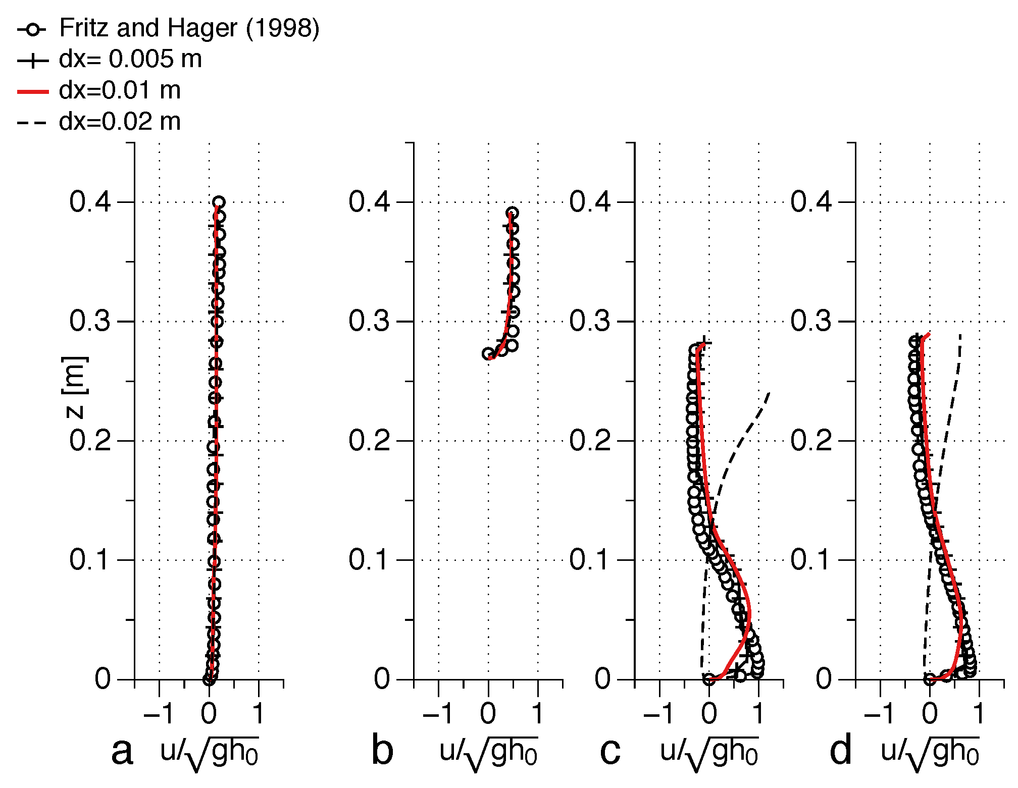
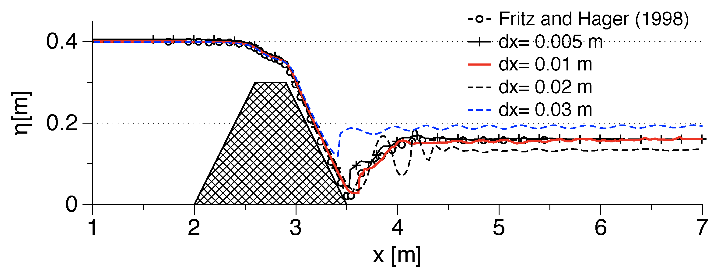
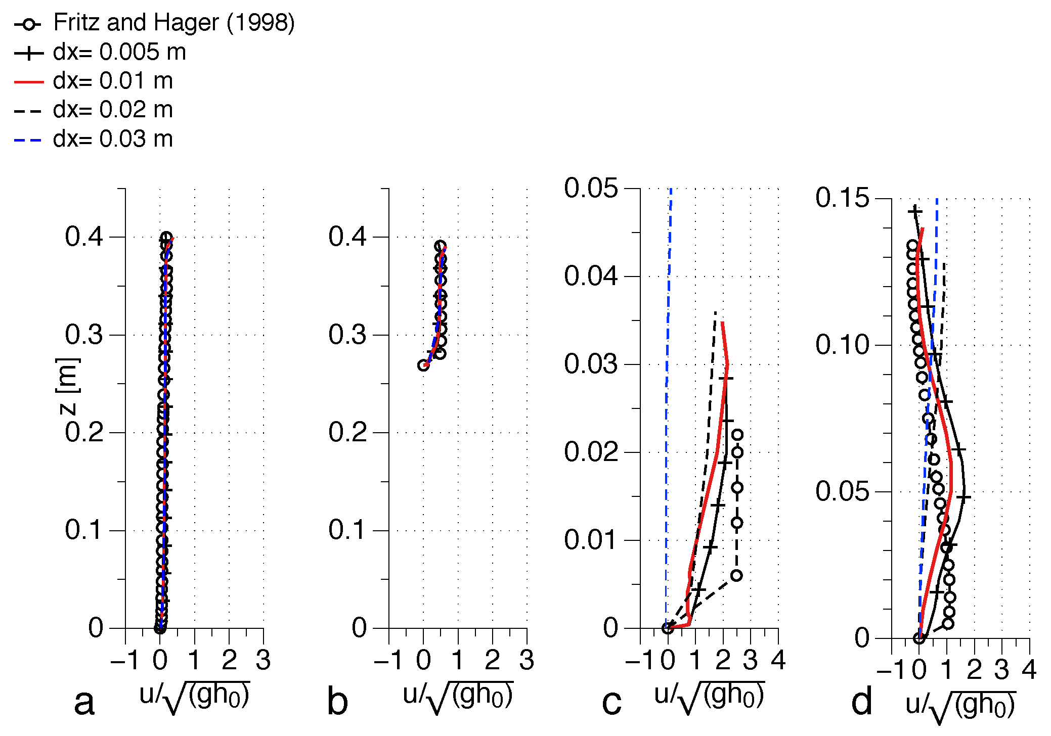
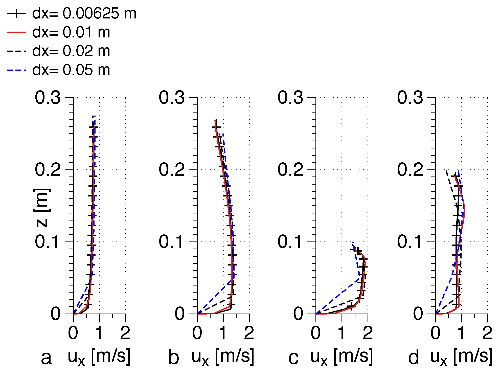
In the first case, submerged overflow on an embankment weir with a surface jet flow and a nearly horizontal free surface is studied. A grid convergence study is carried out for this case with FSTD using m, m and m. The grid convergence for the free surface elevation is presented in Figure 4 and for the stream-wise velocity profiles in Figure 5. The numerical results for the free surface and the velocity profiles are seen to be similar for m and m and the simulation with a grid size of m is used for further analysis of this flow condition.
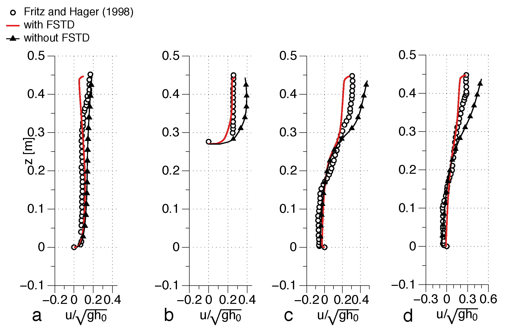
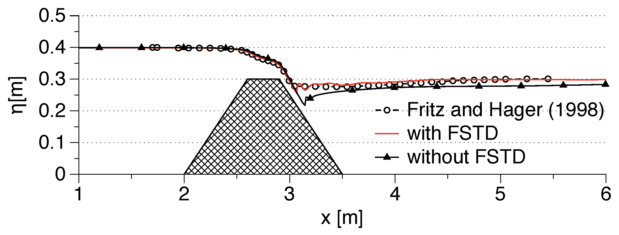
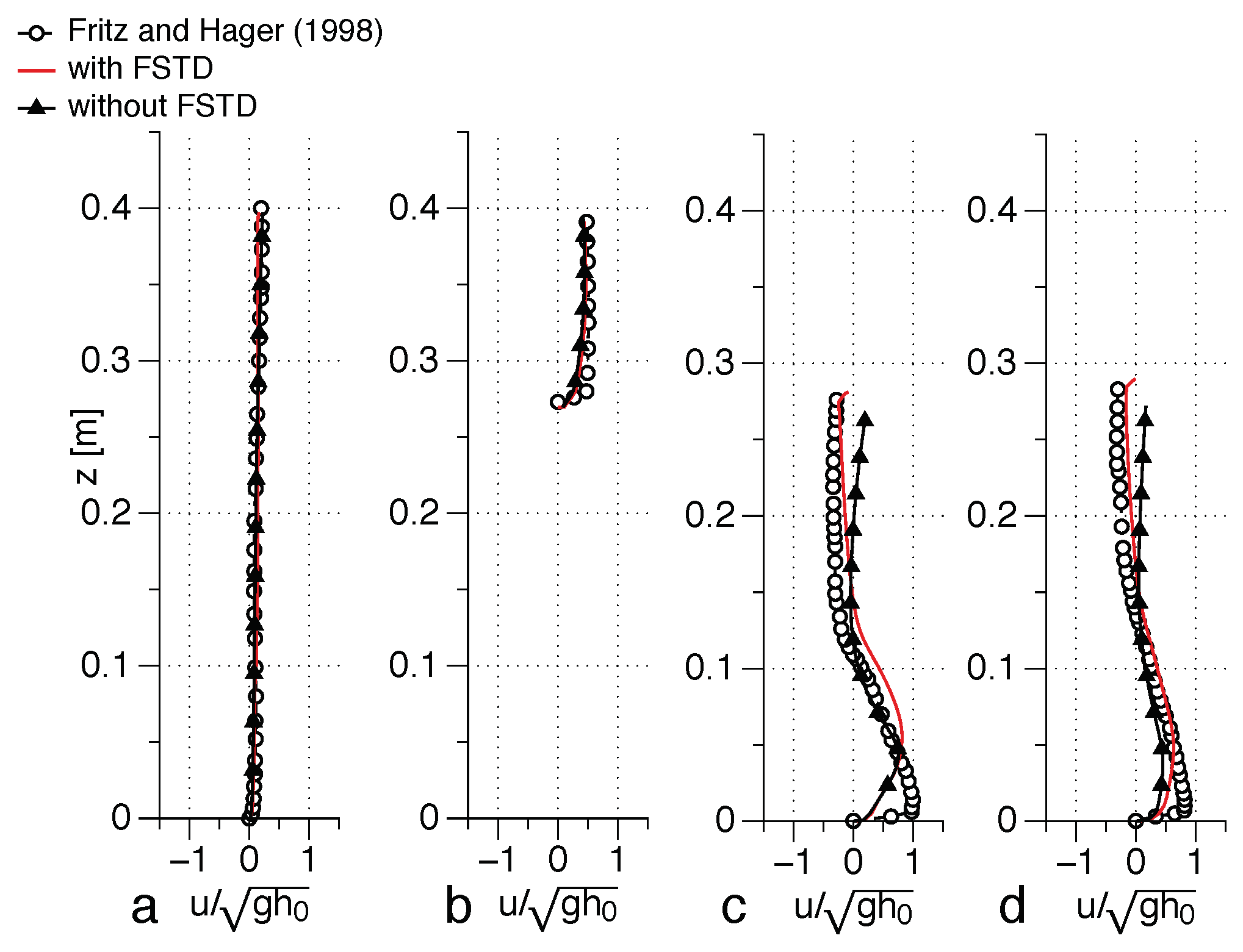
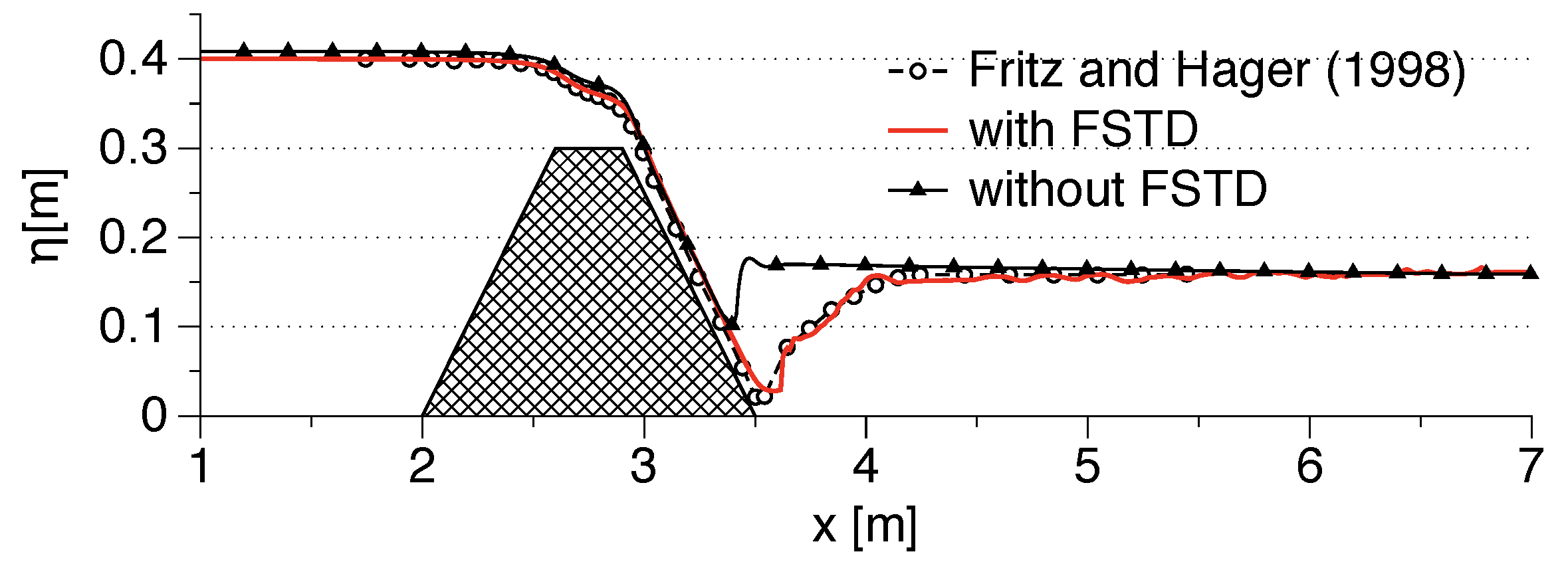
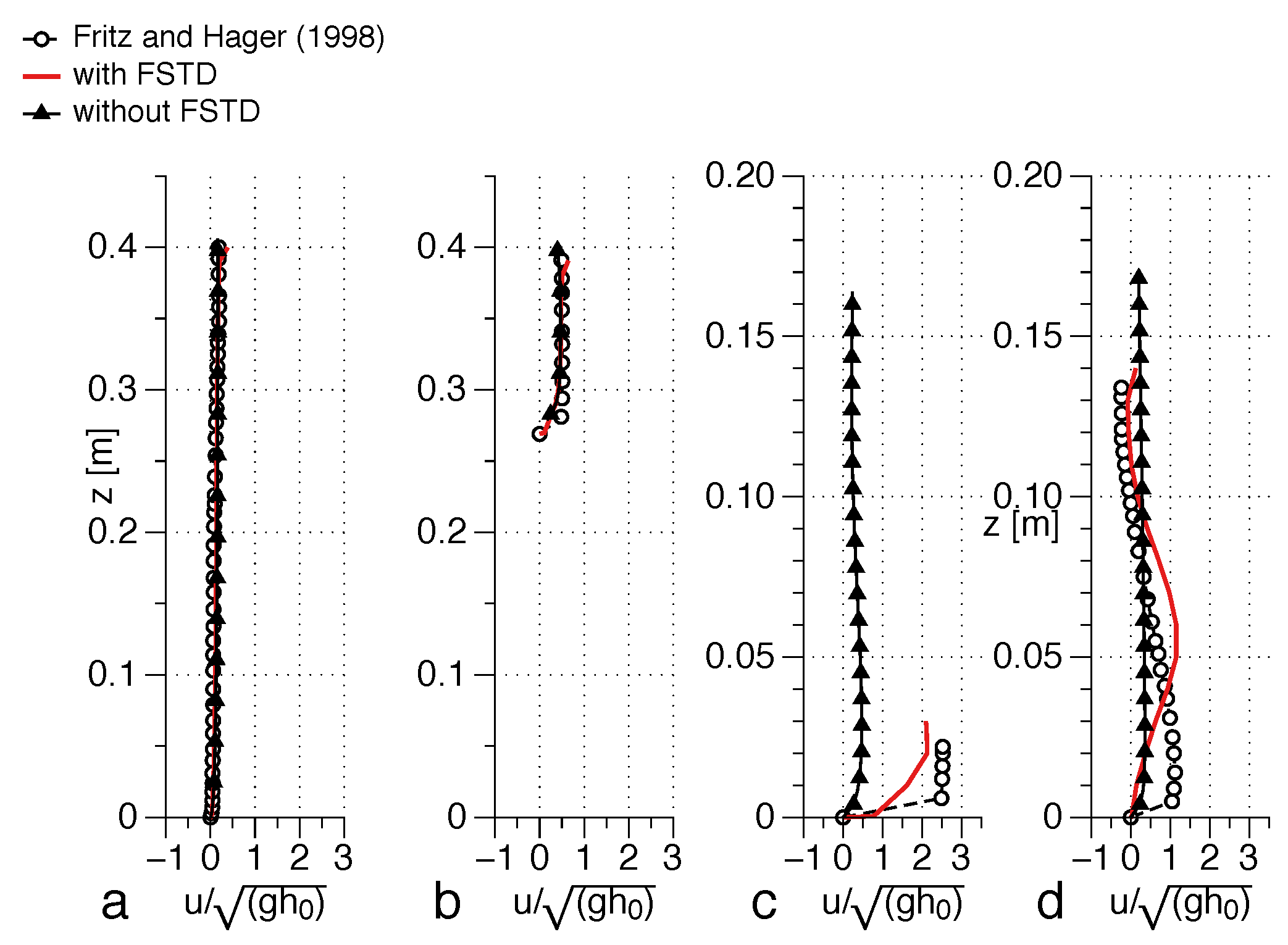
The numerical results for the free surface elevation with and without FSTD are compared to the experimental data in Figure 6. A good agreement is seen between the numerical result with FSTD and the experimental data. The numerical free surface elevation without FSTD in Figure 6 is seen to be similar but slightly lower just downstream of the weir between m and m. Due to the sub-critical flow condition throughout the channel, the free surface has a relatively simple, almost horizontal form and as a result the two simulations show similar results for the free surface elevation. The stream-wise velocity profiles in the simulations with and without FSTD are presented in Figure 7. A large deviation is seen in the velocities closer to the free surface in Figure 7b–d, indicating that the recirculation zones in the flow are calculated differently in the two simulations. The velocity profiles with FSTD show a reasonable agreement with the experimental data.
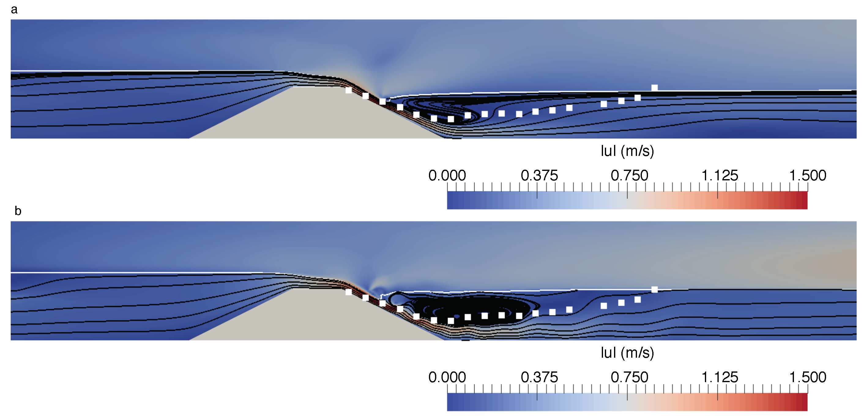
The flow field in the numerical model for this scenario with and without FSTD is presented in Figure 8. The lower limit of the recirculation zone presented by Fritz and Hager [5] is overlaid as white squares on the streamlines to provide a comparison of the recirculation zone calculated in the simulations and the experiments. The streamlines in the water phase in Figure 8a show that while the surface jet is represented, the recirculation zone is over-estimated in the simulation without FSTD. In the simulation with FSTD, the surface jet and the extent of the recirculation zone below the free surface downstream of the embankment weir is correctly represented, as seen from Figure 8b. Thus, despite the numerical free surface elevations in the two simulations being similar, the flow features agree better with the experimental observation in the simulation with FSTD.
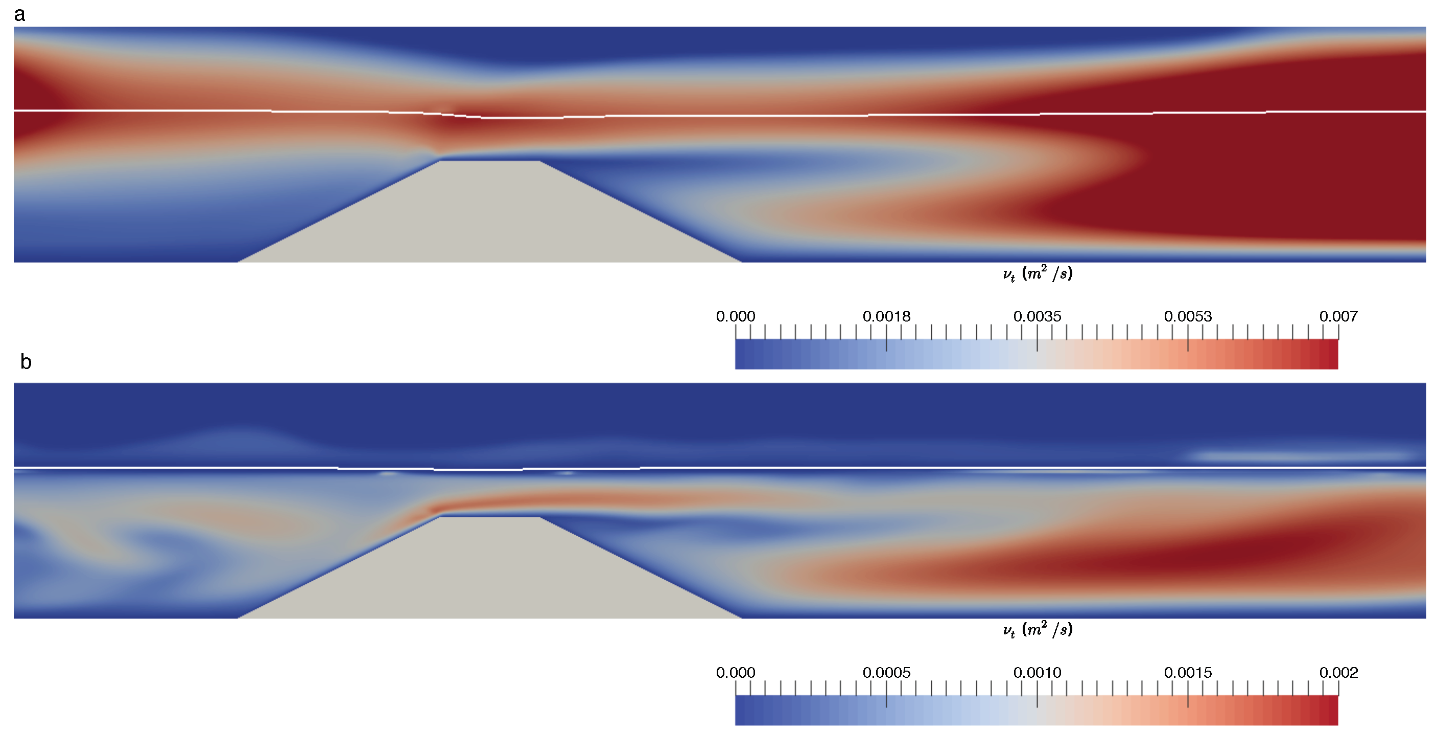
Furthermore, the eddy viscosity in the numerical channel is presented in Figure 9. In the simulation without FSTD, Figure 9a shows that the eddy viscosity has large values around the free surface downstream of the weir, both in the air and water phases. Whereas, in Figure 9b with FSTD, the eddy-viscosity values are much lower around the free surface and higher around the recirculation zone under the free surface and further downstream. Thus, it is seen that even in the simplest case of sub-critical flow throughout the channel, the damping of the turbulence at the free surface significantly aids in the better representation of the flow, even though no significant changes are seen in the calculation of the free surface elevation.
4.1.2. Flow around a Pair of Bridge Piers
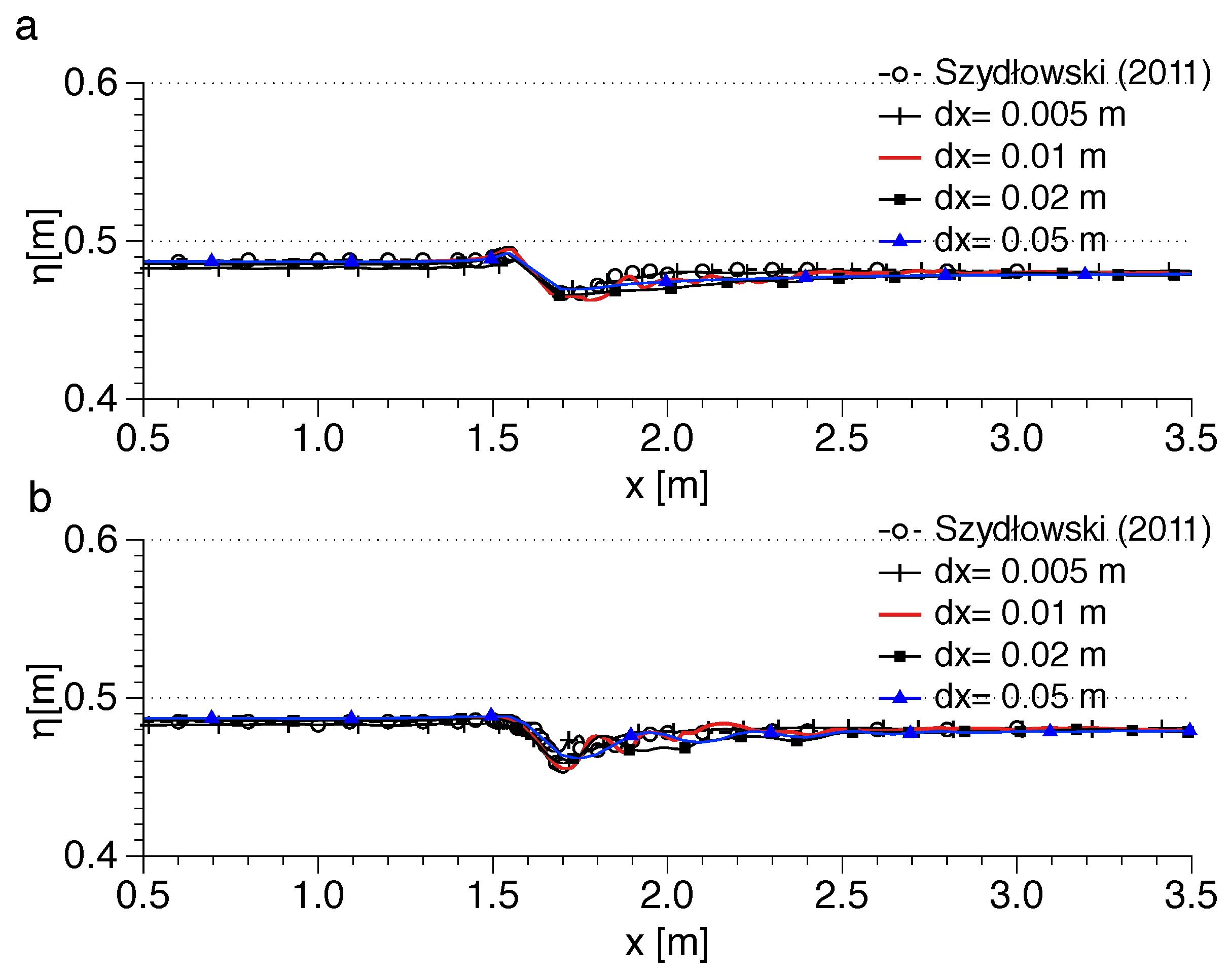
In the second case with sub-critical flow throughout the domain, the flow around a pair of bridge piers is presented. The grid convergence study for the free surface elevation along a line through a pier and along the center of the channel is shown in Figure 10a,b and is seen that the numerical results are similar for all the grid sizes. The results from the simulation with m are used for further analysis. The free surface calculated in simulations with and without FSTD treatment in Figure 11 show that the results are similar. There is a small deflection in the free surface downstream of the piers along the center of the channel which is slightly over-estimated in the simulation without FSTD treatment. The velocity profiles upstream of the piers in Figure 12a at m and Figure 12b at are identical, indicating that the FSTD treatment does not influence the flow upstream of the cylinder. The velocity profile in the vicinity of the deflection at m in Figure 12c shows a difference in the flow field corresponding to the small difference in the location of the free surface at this location. Further downstream from the piers, the velocity profiles at m in Figure 12d, are identical again for the simulations with and without FSTD treatment. The results show that the FSTD treatment has only minor implications for the flow in this case as well.
From the results presented for sub-critical flow throughout the channel with an embankment weir and a pair of bridge piers, it is seen that the representation of the free surface is similar in simulations with and without FSTD treatment. The flow pattern in the vicinity of the structures, on the other hand, can be influenced to some extent. The velocity profiles in the case of the embankment weir with a shallower water depth show a significant difference and consequently the recirculation pattern is not represented correctly without FSTD treatment. In the case of the bridge piers with a higher water depth, the velocity profiles show only a minor difference in the vicinity of the piers.
4.2. Sub-Critical to Super-Critical
In this scenario, the flow condition changes from sub-critical to super-critical after passing the hydraulic structure and stays super-critical until the outflow region. A grid convergence study is carried out for this case with FSTD using m, m, m and m. Figure 13 shows that the most coarse grid with m results in a spurious wave-like flow, which disappears on refining the grid to m. The results for the free surface elevation presented in Figure 13 show that the solution converges at grid size m and this is selected for further analysis of this flow condition.
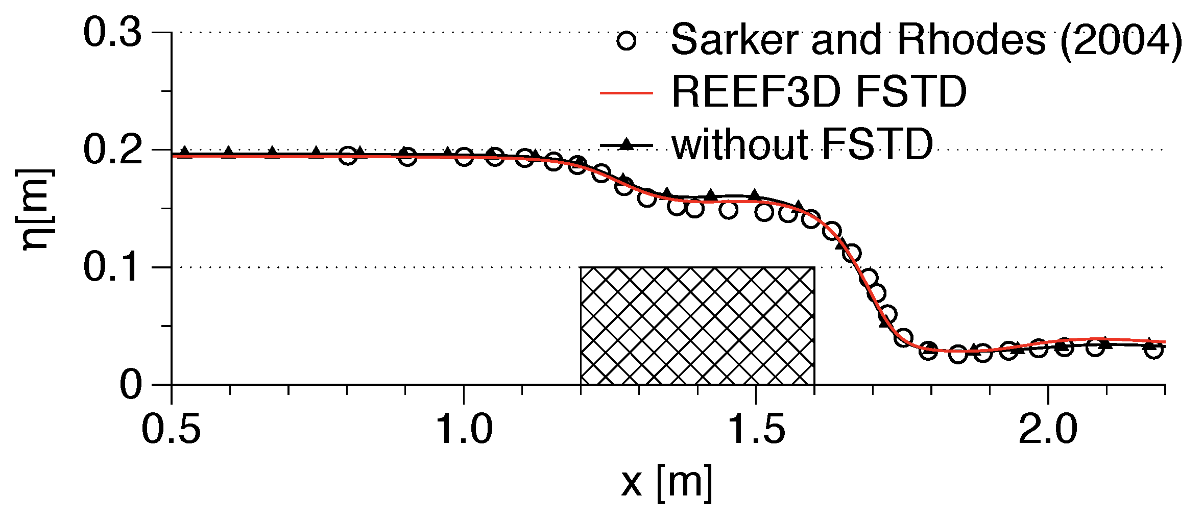
The numerical results with and without FSTD for the free surface elevation are compared to the experimental data from Sarker and Rhodes [41] in Figure 14. The numerical result with FSTD agrees well with the experimental data. Also, the difference in the numerical results for the free surface elevation with and without FSTD is not very significant.
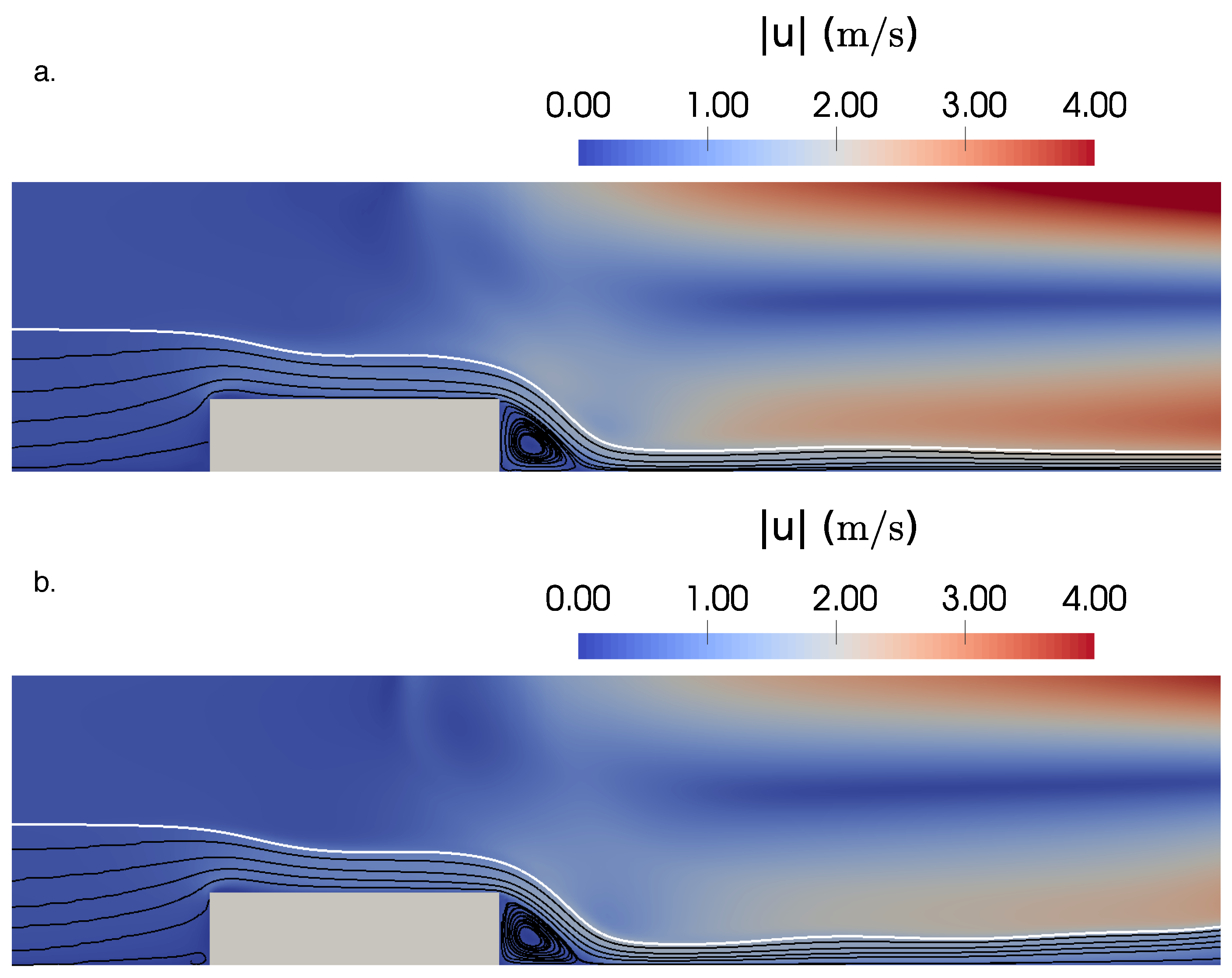
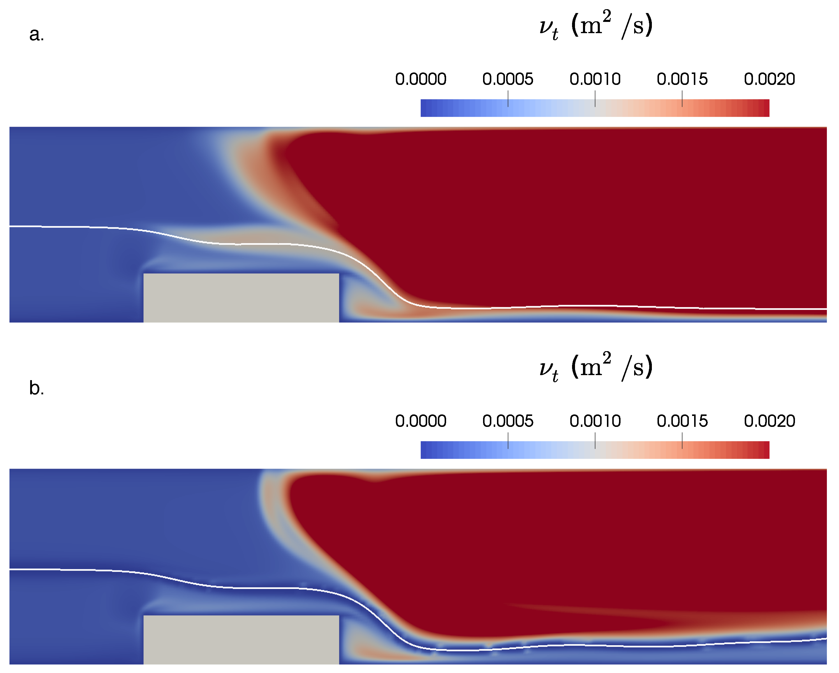
The streamlines and the velocity magnitude contours in the two simulations are shown in Figure 15. It is seen that the extent of the recirculation zone is similar in the two simulations whereas the maximum velocities in the numerical channel are higher in the simulation without FSTD. The distribution of the eddy viscosity along the center of the numerical channel is presented in Figure 16. The higher values of eddy viscosity are distributed around the free surface, in the region with super-critical flow downstream of the weir in Figure 16a for the simulation without FSTD. Whereas in the simulation with FSTD shown in Figure 16b, the higher values of eddy viscosity are found below the free surface and in the recirculation zone downstream of the weir and a region of reduced eddy viscosity around the free surface is clearly seen.
Thus, in the scenario where the flow condition changes from sub-critical to super-critical and stays super-critical until the outlet, the free surface elevation is not changed significantly by FSTD. Some changes are seen in the distribution of the eddy viscosity and the maximum velocity in the channel.
4.3. Transitional Flow
In this section, the flow condition with a plunging jet flow on an embankment weir is presented. The grid convergence study for the free surface elevation in Figure 17 shows that for a coarse grid with m, the plunging jet flow is not represented. With finer grids of m and m the numerical free surface elevation agrees with the experimental data. This is also reflected in the grid convergence study for the stream-wise velocity profiles presented in Figure 18, where the results for m does not agree with the experimental observation downstream of the weir. The velocity profiles for m and m are similar and the results from m are used for further analysis of the flow situation.
The free surface elevations in the simulations with and without FSTD treatment are presented in Figure 19. In the simulation without FSTD, the deflection in the free surface at the location of the plunging jet is over-estimated, whereas in the simulation with FSTD, the free surface agrees with the experimental data. In addition, the free surface further downstream of the weir is underestimated in the simulation without FSTD treatment. The stream-wise velocity profiles in Figure 20a,b show that the calculated flow field is identical upstream of the weir at m and on the upstream face of the weir at m is identical and in agreement with the experimental data. For the velocity profiles on the downstream face of the weir at m and further downstream at m in Figure 20c,d respectively, the numerical results with FSTD agree with the experimental data, whereas without FSTD, the velocities close to the free surface are over-estimated.
The flow in the numerical channel with and without FSTD treatment is investigated using streamlines and the extent of the recirculation zone is compared with the observations in the experiments by Fritz and Hager [5] in Figure 21. While the plunging jet flow is seen in both simulations from the velocity magnitude contours, the recirculation pattern is different in the two simulations. In the simulation without FSTD treatment in Figure 21a, the extent of the recirculation zone is smaller than in the experiments but is correctly represented in the simulation with FSTD as seen in Figure 21b. The eddy viscosity in the simulation without FSTD treatment is seen to have very high values around the free surface in Figure 22a. The FSTD treatment results in lower turbulent production around the interface as seen in Figure 22b.
From the results for the transitional flow regime with a plunging jet flow on an embankment weir, it is seen that the difference in the calculation of the free surface and the recirculation pattern is significantly influenced by the over-production of turbulence around the free surface in the absence of the FSTD algorithm. This contrasts with the flow scenarios with sub-critical flow throughout the channel and sub-critical to super-critical flow transition presented in the previous sections, where the difference in the numerical results are generally smaller with and without the application of FSTD.
4.4. Sub-Critical to Super-Critical to Sub-Critical
This is the most complex flow scenario simulated in this study where the flow conditions change from sub-critical to super-critical and back to sub-critical in the vicinity of the hydraulic structure. Two cases are presented for this scenario, the first case is the free overflow over an embankment weir presented by Fritz and Hager [5] and the second case is the flow around a pair of bridge piers presented by Szydłowski [40].
4.4.1. Flow over an Embankment Weir
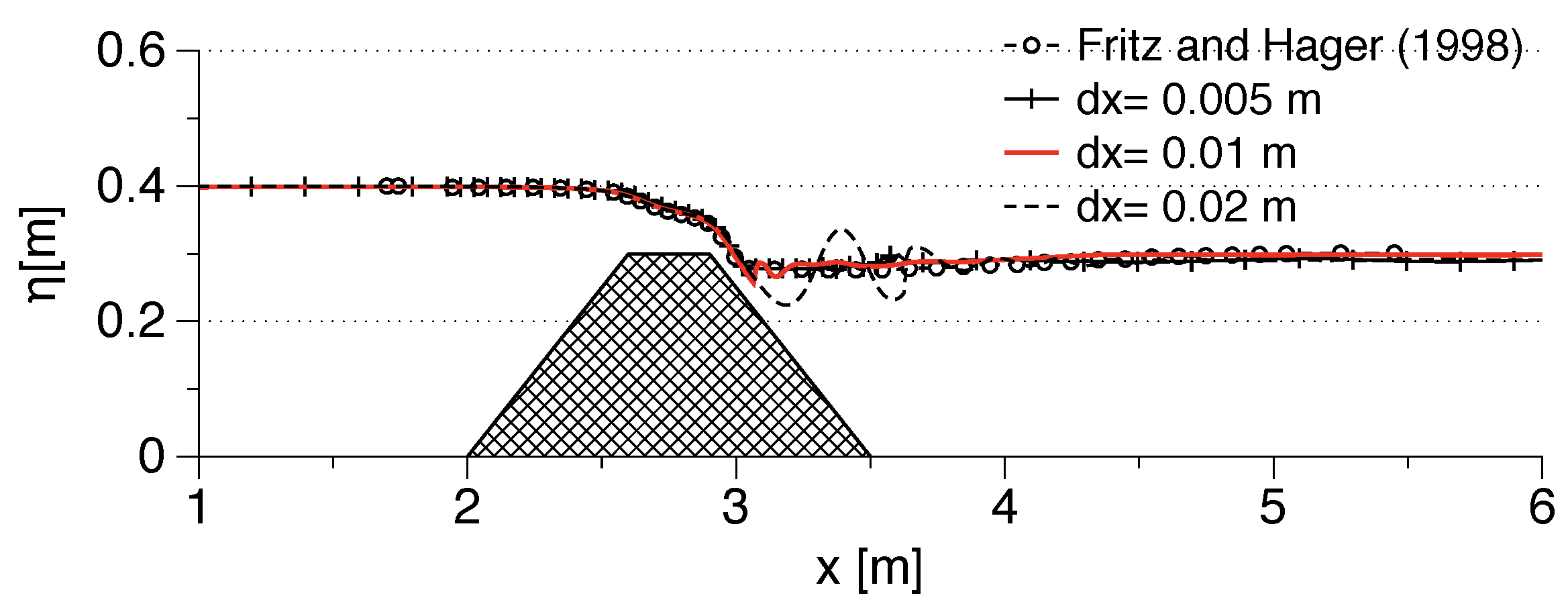
A grid convergence study is carried out with FSTD using m, m, m and m. The results for the free surface elevation shown in Figure 23. For the coarse grid with m, the hydraulic jump is not represented, and additional waves are seen downstream of the weir for m. The numerical results improve with grid refinement and the free surface elevation with m and m are seen to be similar and agree with the experimental data. The grid convergence study for the stream-wise velocity profile is presented in Figure 24. The velocity profiles are identical upstream of the weir at m, and on the upstream face of the weir at m for all the grid sizes in Figure 24a,b, respectively. At the location of the hydraulic jump at m and further downstream at m in Figure 24c,d respectively, the velocity profiles for m and m are similar. The results from m are used for further analysis of the case.
The numerical result for the free surface elevation with and without FSTD is compared to the experimental data in Figure 25. The numerical result with FSTD agrees with the experimental data, including the representation of the hydraulic jump. The difference between the calculated free surface elevations in the simulations with and without FSTD is clearly seen. The free surface elevation returns to the tailwater level sharply downstream of the weir and has a constant free surface in the simulation without FSTD. The stream-wise velocity profiles show that the flow field is similar upstream of the weir in Figure 26a,b respectively with and without FSTD. The velocity profile at the location of the hydraulic jump in Figure 26c shows a significant difference between the two simulations corresponding to the difference in the free surface location. The velocity profile in the simulation with FSTD follows the observations from the experiments, though a slight overestimation of the free surface location by about m and a corresponding deviation from the experimental observation is seen in Figure 26c. Further downstream of the weir at m in Figure 26d, the over-estimated horizontal free surface in the simulation without FSTD corresponds to a different velocity profile, while the result with FSTD treatment is closer to the experimental observation.
The lower limit of the recirculation zone presented by Fritz and Hager [5] is overlaid as white squares on the streamlines to provide a comparison of the recirculation zone calculated in the simulations in Figure 27. The streamlines and the velocity magnitude contours in Figure 27a show that the recirculation zone and the submerged flow are not calculated in the simulation without FSTD. The simulation with FSTD in Figure 27b shows that the calculated recirculation region agrees well with the lower limit of the recirculation zone in the experiments. The distribution of the eddy viscosity in the channel for the two simulations is presented in Figure 28. In the simulation without FSTD, the higher values of eddy viscosity are located around the free surface, in the region of the hydraulic jump. This has a damping effect on the flow in the region and the hydraulic jump is not represented correctly as seen in Figure 28a. In the simulation with FSTD in Figure 28b, the values of eddy viscosity are the lowest just around the free surface.
Thus, it is clearly seen from this case that the FSTD treatment has a significant effect on the calculation of the free surface elevation and the flow features involved in a scenario where the flow conditions undergo rapid changes from sub-critical to super-critical and back to sub-critical. The representation of the free surface elevation and the recirculation zone is more realistic in the simulations with FSTD as seen from the comparisons with the experimental results.
4.4.2. Flow around a Pair of Bridge Piers
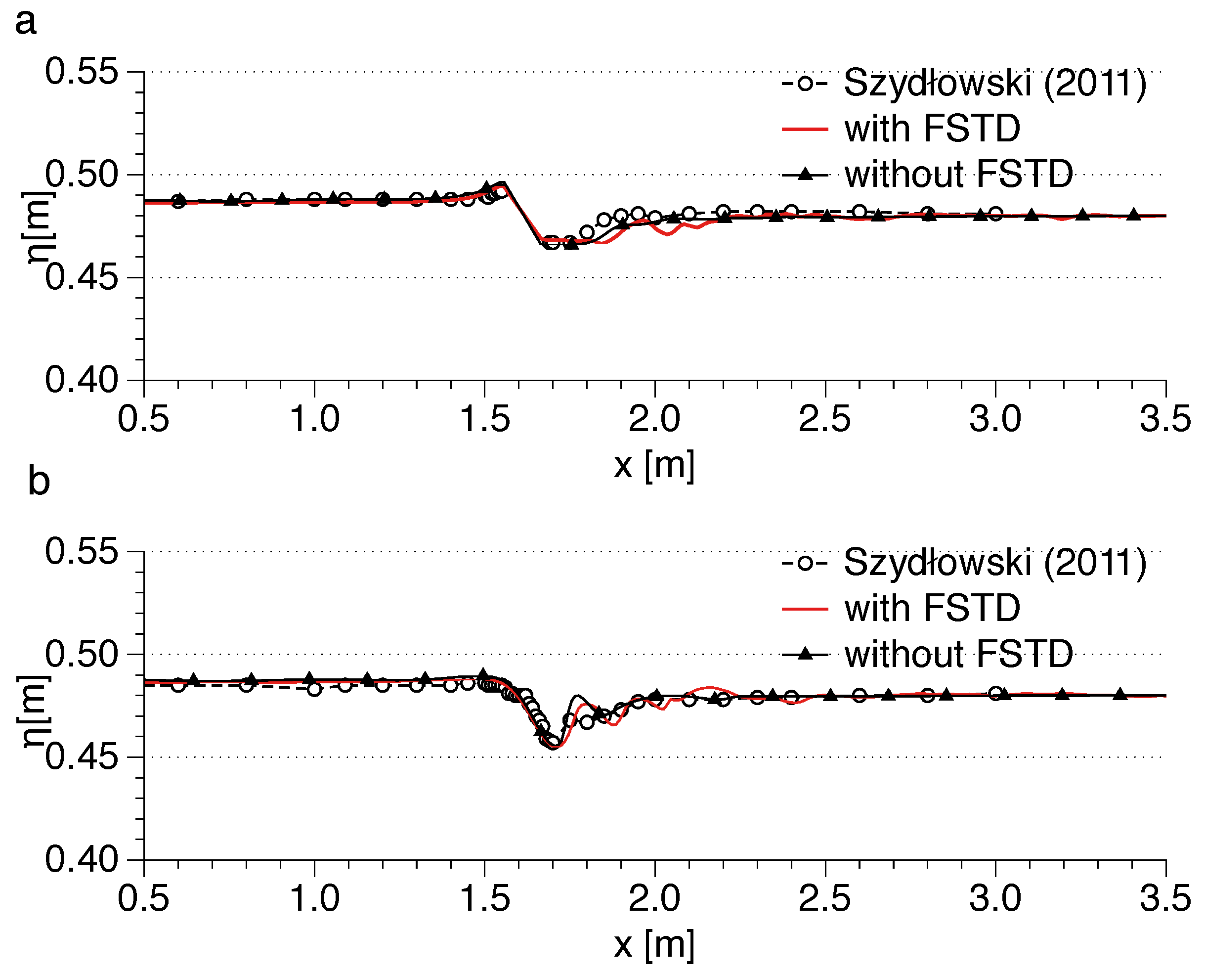
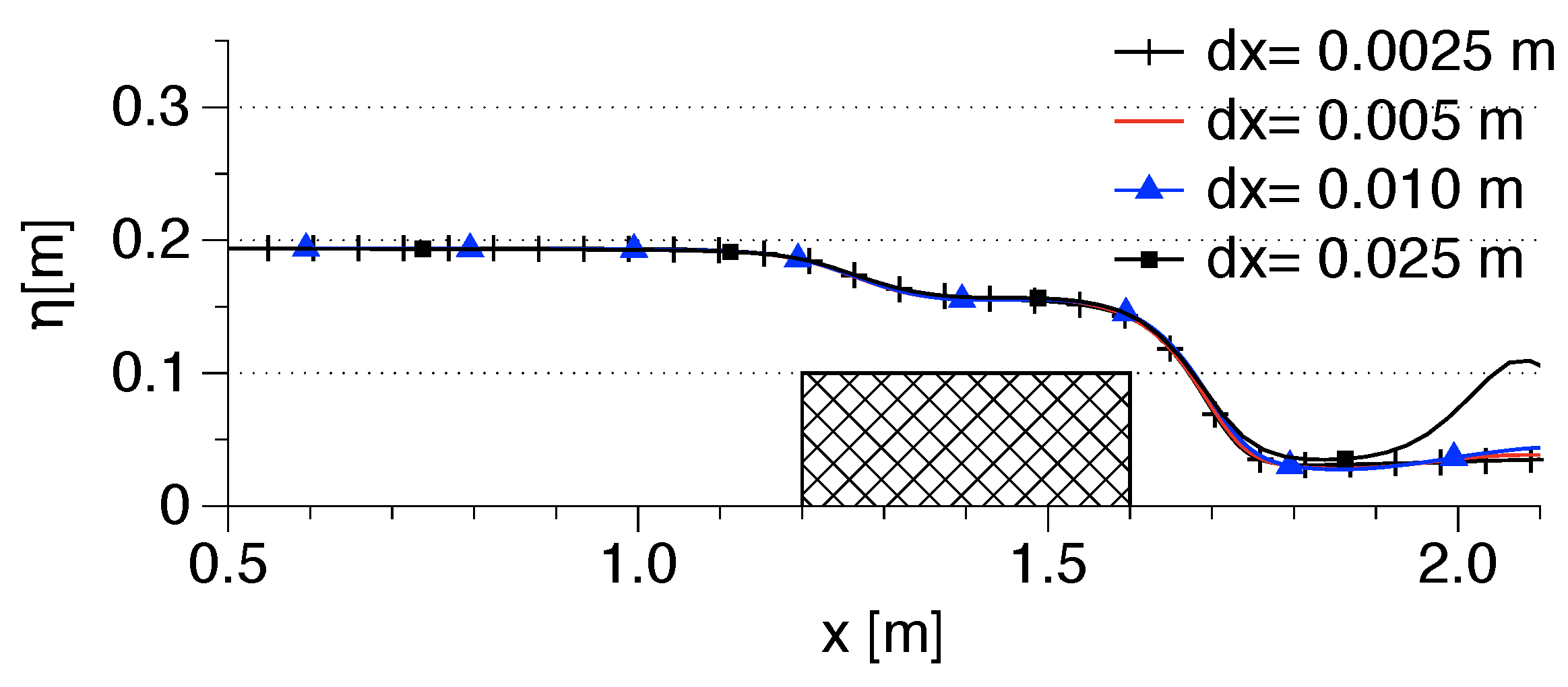
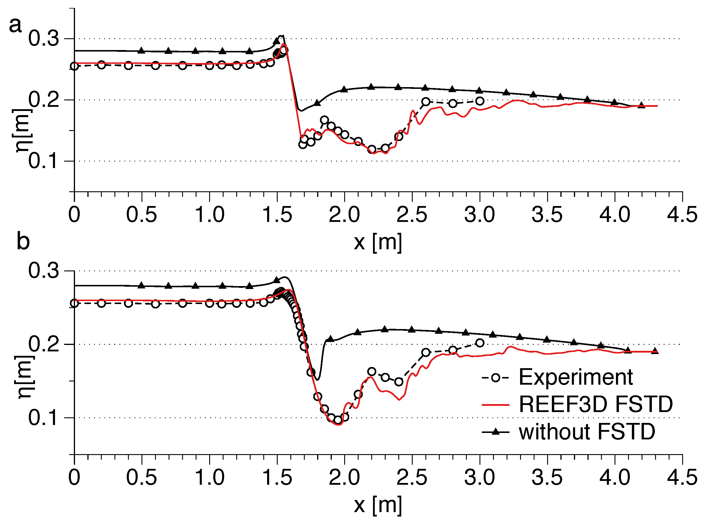
A grid convergence study is carried out in this case using grid sizes m, m, m, m and m using FSTD in the simulations. The results for the free surface along the center of the channel (m) and along the center line through a pier ( m) are presented in Figure 29. The free surface elevations agree with the experimental data for m and m with the hydraulic jump correctly represented in the numerical result. The grid convergence study for the stream-wise velocity profiles in Figure 30 shows that the numerical results improve with grid refinement and similar values are obtained with m and m. The results obtained with the grid size of m are used in the analysis of this flow condition.
The obstruction due to the bridge piers leads to super-critical flow downstream of the piers and the flow regime changes back to sub-critical near the outflow. The comparison of the numerical results with experimental data in this case with and without FSTD along the center line through a pier ( m) is shown in Figure 31a and along the center of the channel ( m) is presented in Figure 31b. These results show the importance of FSTD in complex flow situations. The free surface downstream of the piers is elevated and the free surface in the super-critical region is not represented correctly both along the center of the channel and along the center line through one of the piers without FSTD. The free surface downstream of the piers slopes downwards towards the outlet to meet the controlled outflow boundary condition. This together with the elevated free surface upstream of the piers indicates an unphysical energy loss in the numerical channel due to the over-production of eddy viscosity around the free surface. On the other hand, in the numerical results with FSTD follow the experimental data all along the channel including the hydraulic jump and the slope of the downstream free surface does not have a distinct slope towards the outlet.
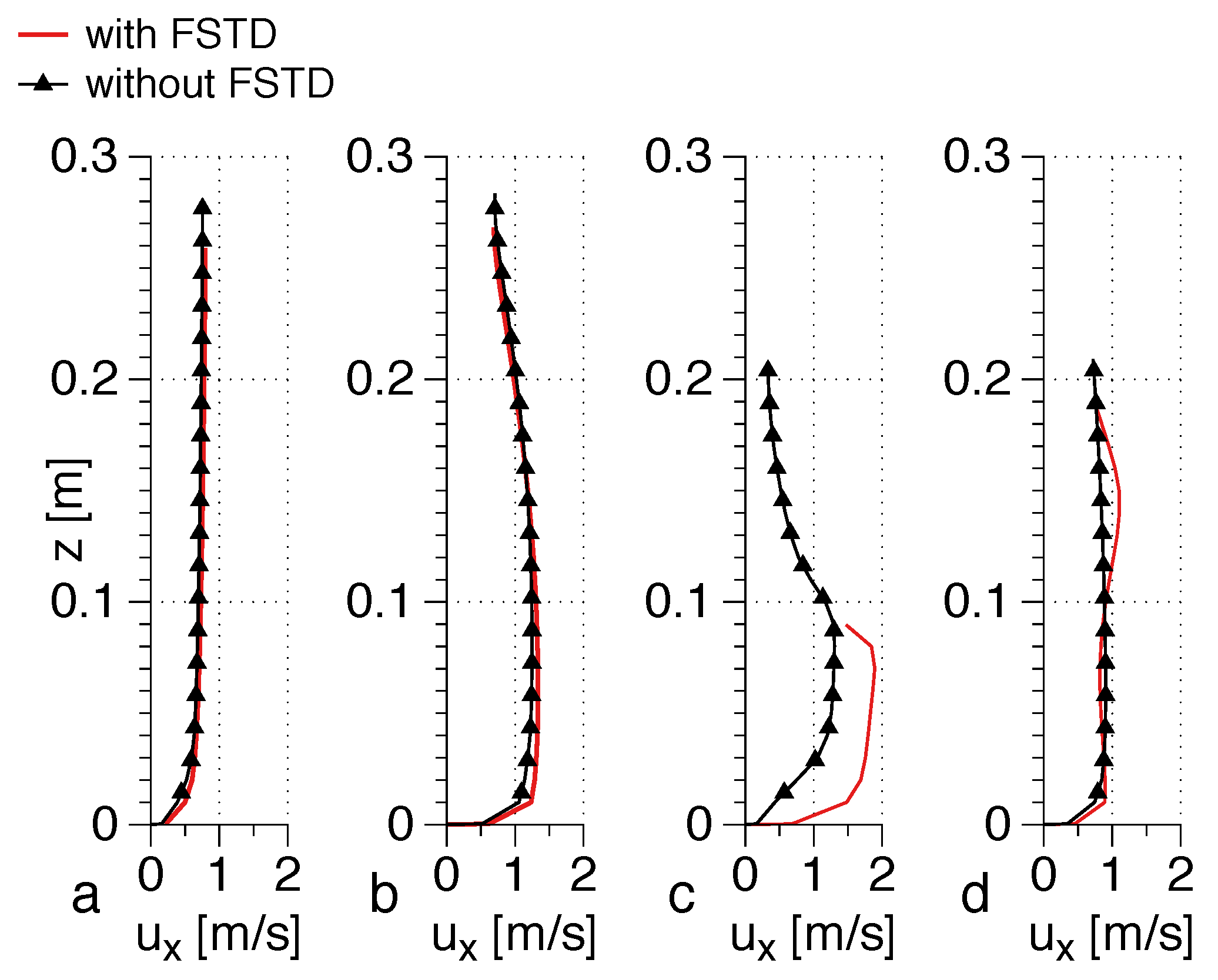
The stream-wise velocity profiles with and without FSTD at various locations in the channel show that the flow field is similar upstream of the piers at m and between the piers at m in Figure 32a,b, respectively. The major difference is seen in Figure 32c at the trough of the hydraulic jump at m. The application of FSTD results in a more physical distribution of the horizontal velocity along the water depth and the maximum horizontal velocity is seen just under the free surface. In the absence of FSTD, the free surface is higher, and the maximum horizontal velocity occurs much below the free surface. Further downstream at m in Figure 32, the velocity profiles differ only in the vicinity of the free surface, corresponding to the small difference in the free surface elevation.
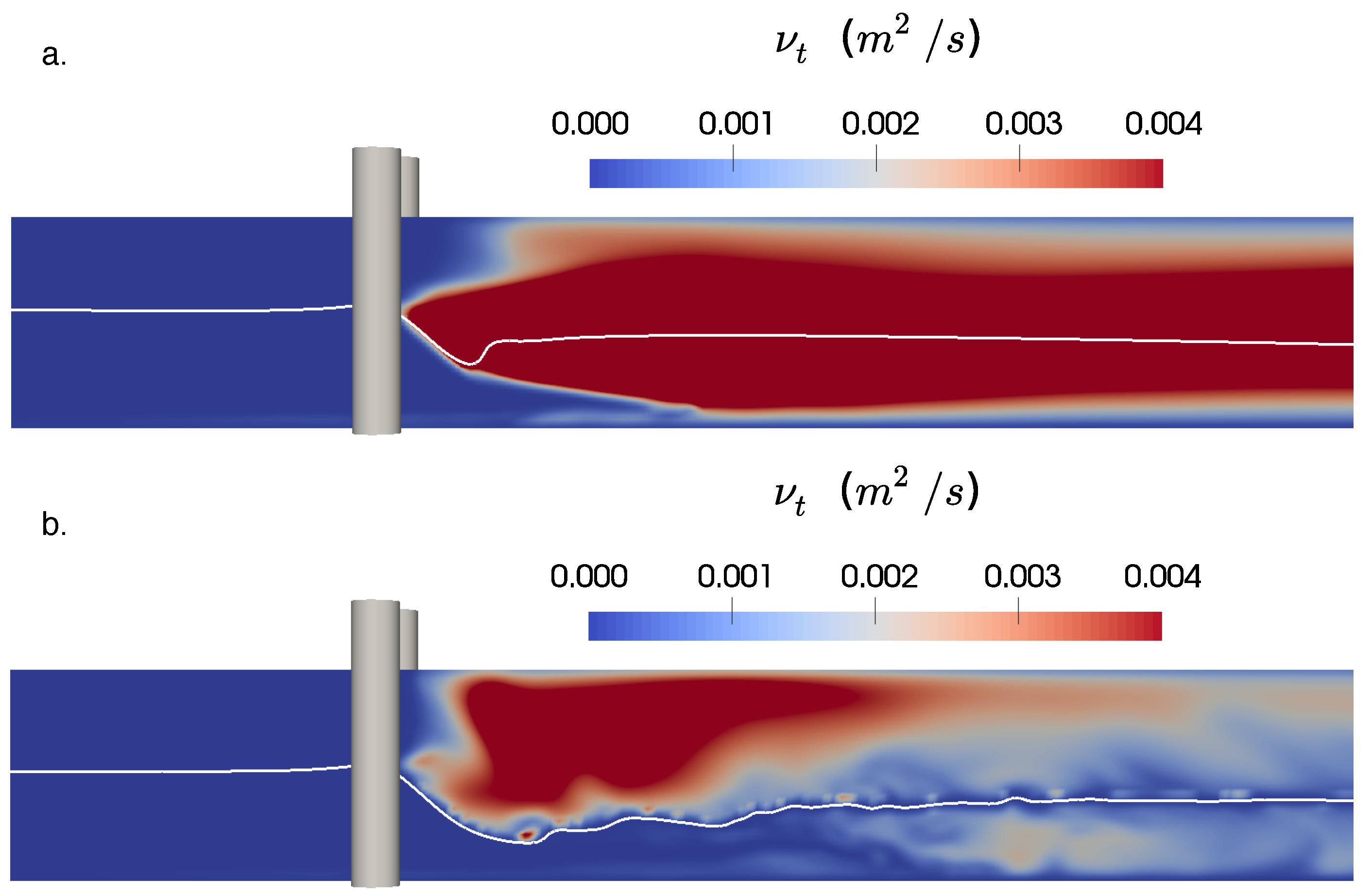
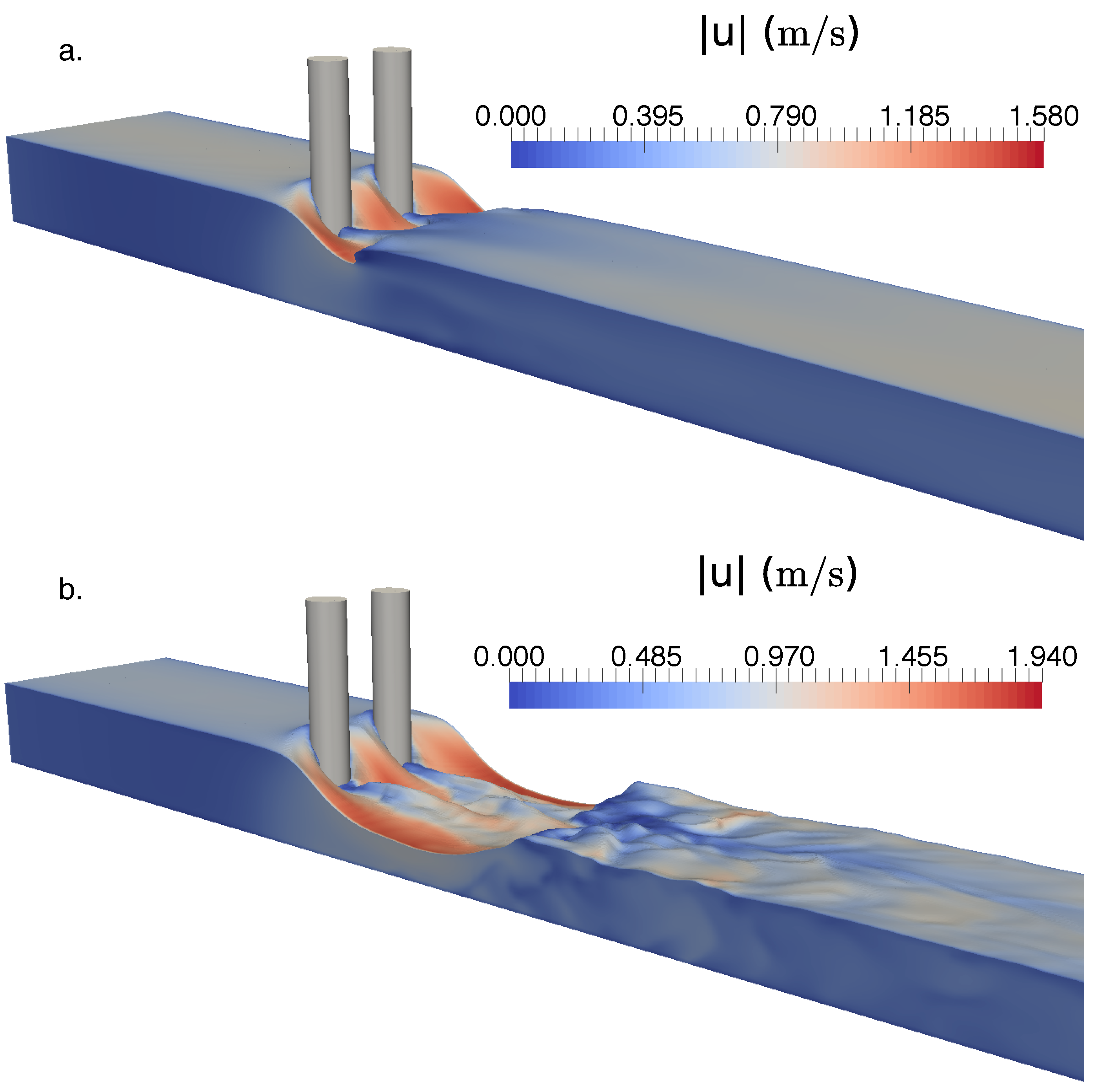
The difference between the flow regimes in the two simulations is further demonstrated with the eddy viscosity in the channel. Figure 33 shows the eddy-viscosity distribution around the free surface without and with FSTD. Without FSTD, high values are seen for the eddy viscosity around the free surface especially in the region of the hydraulic jump behind the piers in Figure 33a. The strain in the flow at this location is the highest in the channel due to the occurrence of the hydraulic jump. The highly strained flow results in an unphysical high value of eddy viscosity in the region, resulting in a damped out free surface. On the other hand, with FSTD, the eddy viscosity around the interface is reduced in Figure 33b and the free surface resembles the experimental observations. The flow in the channel and the free surface features in the three-dimensional numerical channel without FSTD is shown in Figure 34a shows the abrupt jump in the free surface downstream of the piers and the horizontal free surface further downstream. In the simulation with FSTD in Figure 34b, the region downstream of the piers shows a rapid decrease in free surface elevation with a trans-critical flow, the formation of a hydraulic jump and the flow returns to a sub-critical flow further downstream.
The results presented above for a rapidly varying flow situation from sub-critical to super-critical and back to sub-critical with the free surface elevations, velocity profiles, the recirculation zone and the distribution of the eddy viscosity show that the application of a FSTD algorithm is essential to obtain realistic and physical results in such cases using immiscible two-phase RANS equations.
5. Conclusions
The open-source CFD model REEF3D is used to simulate free surface flows around different hydraulic structures with different flow conditions using immiscible two-phase RANS equations. The distribution of the eddy viscosity, the velocity magnitude, and the recirculation zones in the numerical channel are analyzed for the different cases and compared to experimental data and correlated with the effect of FSTD treatment. From the investigation of the different flow scenarios presented in this study, the following conclusions can be drawn:
- When the flow conditions remain sub-critical throughout the domain, the calculated free surface elevations are similar with and without FSTD but the submerged recirculation zone is better represented when FSTD is used.
- When the flow conditions change from sub-critical to super-critical, the calculated free surface elevation and the flow features such as the recirculation zone are similar with and without FSTD.
- In the case of transitional flow, the differences in the calculation of the free surface and the recirculation pattern become more apparent.
- When the flow conditions change from sub-critical to super-critical and back to sub-critical, the calculated free surface elevation and the flow features such as the hydraulic jump and the recirculation zone are represented correctly only in the simulation with FSTD.
- In general, simulations with FSTD provide a more physical representation of the recirculation zone. The calculation of free surface elevation is significantly affected in the complex case of flow conditions changing from sub-critical to super-critical to sub-critical.
The results demonstrate the importance of FSTD treatment in immiscible two-phase RANS simulations of flow around hydraulic structures. The implementation also addresses an important issue of over-production of turbulence at the free surface in two-phase RANS modelling during complex free surface flow using an empirical approach that is based on the flow physics. The proposed boundary condition is shown to be numerically stable in all the flow situations studied and has varying degree of influence on the results, depending in the flow situation. It is also demonstrated that two-phase RANS modelling that does not resolve the detailed eddies in turbulent flow can be used to obtain reasonably accurate representation of complex flow conditions. In the case of flows with hydraulic jumps, the internal structures of the flow and the air entrainment are not presented, but the bulk quantities that influence engineering design of hydraulic structures such as the free surface and the velocity profile over depth are well represented. This provides an alternative tool to analyze engineering design of hydraulic structures at a computational expense that is much lower than that required by eddy-resolving models.
Author Contributions
Lead Author A.K. was responsible for the design of the simulations, compilation of the results and drafting the manuscript. G.F. carried out initial testing and validation. Concept development, coding and academic supervision by H.B.
Funding
This research received no external funding.
Acknowledgments
The authors thank Michał Szydłowski for providing the experimental data for the free surface elevations for the flow scenario with the bridge piers. GF was supported through the ÚNKP-18-3-I New National Excellence Program of the Ministry of Human Capacities. This research was supported in part with computational resources at the Norwegian University of Science and Technology (NTNU) provided by NOTUR (No. NN2620K), http://www.notur.no.
Conflicts of Interest
The authors declare no conflict of interest.
References
- Rouse, H.; Bhoota, B.; Hsu, E.Y. Design of Channel Expansion. Proc. Am. Soc. Civ. Eng. (ASCE) 1951, 75, 1369–1385. [Google Scholar]
- Ippen, A.T.; Dawson, J.H. Design of channel contractions. Proc. Am. Soc. Civ. Eng. (ASCE) 1951, 75, 1348–1368. [Google Scholar]
- Hager, W.H. Supercritical flow in channel junctions. J. Hydraul. Eng. 1989, 115, 595–616. [Google Scholar] [CrossRef]
- Mazumder, S.K.; Hager, W.H. Supercritical expansion flow in Rouse modified and reversed transitions. J. Hydraul. Eng. 1993, 119, 201–219. [Google Scholar] [CrossRef]
- Fritz, H.M.; Hager, W.H. Hydraulics of embankment weirs. J. Hydraul. Eng. 1998, 124, 963–971. [Google Scholar] [CrossRef]
- Tullis, B.; Neilson, J. Performance of submerged ogee-crest weir head-discharge relationships. J. Hydraul. Eng. 2008, 134, 486–491. [Google Scholar] [CrossRef]
- Murzyn, F.; Chanson, H. Free-surface fluctuations in hydraulic jumps: Experimental observations. Exp. Therm. Fluid Sci. 2009, 33, 1055–1064. [Google Scholar] [CrossRef]
- Chachereau, Y.; Chanson, H. Free-surface fluctuations and turbulence in hydraulic jumps. Exp. Therm. Fluid Sci. 2011, 35, 896–909. [Google Scholar] [CrossRef]
- Brunner, G.W. HEC-RAS (River Analysis System). In Proceedings of the North American Water and Environment Congress & Destructive Water, Anaheim, CA, USA, 22–28 June 1996; pp. 3782–3787. [Google Scholar]
- Olsen, N. A Three Dimensional Numerical Model for Simulation of Sediment Movements in Water Intakes with Multiblock Option: Version 1.1 and 2.0 User’s Manual; Department of Hydraulic and Environmental Engineering, The Norwegian University of Science and Technology: Trondheim, Norway, 2003; p. 138. [Google Scholar]
- Haun, S.; Olsen, N.R.B.; Feurich, R. Numerical modeling of flow over trapezoidal broad-crested weir. Eng. Appl. Comput. Fluid Mech. 2011, 5, 397–405. [Google Scholar] [CrossRef]
- Fleit, G.; Baranya, S.; Bihs, H. CFD Modeling of Varied Flow Conditions Over an Ogee-Weir. Period. Polytech. Civ. Eng. 2017, 1–7. [Google Scholar] [CrossRef]
- Kirkil, G.; Constantinescu, S.G.; Ettema, R. Coherent structures in the flow field around a circular cylinder with scour hole. J. Hydraul. Eng. 2008, 134, 572–587. [Google Scholar] [CrossRef]
- Kara, S.; Kara, M.C.; Stoesser, T.; Sturm, T.W. Free-surface versus rigid-lid LES computations for bridge-abutment flow. J. Hydraul. Eng. 2015, 141, 04015019. [Google Scholar] [CrossRef]
- Kang, S.; Sotiropoulos, F. Large-eddy simulation of three-dimensional turbulent free surface flow past a complex stream restoration structure. J. Hydraul. Eng. 2015, 141, 04015022. [Google Scholar] [CrossRef]
- McSherry, R.J.; Chua, K.V.; Stoesser, T. Large eddy simulation of free-surface flows. J. Hydrodyn. Ser. B 2017, 29, 1–12. [Google Scholar] [CrossRef]
- Viti, N.; Valero, D.; Gualtieri, C. Numerical Simulation of Hydraulic Jumps. Part 2: Recent Results and Future Outlook. Water 2019, 11, 28. [Google Scholar] [CrossRef]
- Jacobsen, N.G.; Fuhrman, D.R.; Fredsøe, J. A wave generation toolbox for the open-source CFD library: OpenFOAM. Int. J. Numer. Methods Fluids 2012, 70, 1073–1088. [Google Scholar] [CrossRef]
- Devolder, B.; Rauwoens, P.; Troch, P. Application of a buoyancy-modified SST turbulence model to simulate wave run-up around a monopile subjected to regular waves using OpenFOAM®. Coast. Eng. 2017, 125, 81–94. [Google Scholar] [CrossRef]
- Larsen, B.E.; Fuhrman, D.R. On the over-production of turbulence beneath surface waves in Reynolds-averaged Navier-Stokes models. J. Fluid Mech. 2018, 853, 419–460. [Google Scholar] [CrossRef]
- Naot, D.; Rodi, W. Calculation of secondary currents in channel flow. J. Hydraul. Div. ASCE 1982, 108, 948–968. [Google Scholar]
- Bihs, H.; Kamath, A.; Alagan Chella, M.; Aggarwal, A.; Arntsen, Ø.A. A new level set numerical wave tank with improved density interpolation for complex wave hydrodynamics. Comput. Fluids 2016, 140, 191–208. [Google Scholar] [CrossRef]
- Kamath, A.; Bihs, H.; Alagan Chella, M.; Arntsen, Ø.A. Upstream-Cylinder and Downstream-Cylinder Influence on the Hydrodynamics of a Four-Cylinder Group. J. Waterw. Port Coast. Ocean Eng. 2016, 142, 04016002. [Google Scholar] [CrossRef]
- Kamath, A.; Alagan Chella, M.; Bihs, H.; Arntsen, Ø.A. Breaking wave interaction with a vertical cylinder and the effect of breaker location. Ocean Eng. 2016, 128, 105–115. [Google Scholar] [CrossRef]
- Bihs, H.; Kamath, A.; Alagan Chella, M.; Arntsen, Ø.A. Breaking-Wave Interaction with Tandem Cylinders under Different Impact Scenarios. J. Waterw. Port Coast. Ocean Eng. 2016, 142, 04016005. [Google Scholar] [CrossRef]
- Alagan Chella, M.; Bihs, H.; Myrhaug, D.; Muskulus, M. Breaking solitary waves and breaking wave forces on a vertically mounted slender cylinder over an impermeable sloping seabed. J. Ocean Eng. Mar. Energy 2017, 3, 1–19. [Google Scholar] [CrossRef]
- Bihs, H.; Kamath, A. A combined level set/ghost cell immersed boundary representation for floating body simulations. Int. J. Numer. Methods Fluids 2017, 83, 905–916. [Google Scholar] [CrossRef]
- Chorin, A. Numerical solution of the Navier-Stokes equations. Math. Comput. 1968, 22, 745–762. [Google Scholar] [CrossRef]
- Ashby, S.F.; Falgout, R.D. A Parallel Mulitgrid Preconditioned Conjugate Gradient Algorithm for Groundwater Flow Simulations. Nucl. Sci. Eng. 1996, 124, 145–159. [Google Scholar] [CrossRef]
- Center for Applied Scientific Computing. HYPRE High Performance Preconditioners—User’s Manual; Lawrence Livermore National Laboratory: Livermore, CA, USA, 2006. [Google Scholar]
- Wilcox, D.C. Turbulence Modeling for CFD; DCW Industries Inc.: La Canada, CA, USA, 1994. [Google Scholar]
- Durbin, P.A. Limiters and wall treatments in applied turbulence modeling. Fluid Dyn. Res. 2009, 41, 1–18. [Google Scholar] [CrossRef]
- Hossain, M.S.; Rodi, W. Mathematical modeling of vertical mixing in stratified channel flow. In Proceedings of the 2nd Symposium on Stratified Flows, Trondheim, Norway, 24–27 June 1980. [Google Scholar]
- Osher, S.; Sethian, J.A. Fronts propagating with curvature-dependent speed: Algorithms based on Hamilton-Jacobi formulations. J. Comput. Phys. 1988, 79, 12–49. [Google Scholar] [CrossRef]
- Peng, D.; Merriman, B.; Osher, S.; Zhao, H.; Kang, M. A PDE-based fast local level set method. J. Comput. Phys. 1999, 155, 410–438. [Google Scholar] [CrossRef]
- Jiang, G.S.; Shu, C.W. Efficient implementation of weighted ENO schemes. J. Comput. Phys. 1996, 126, 202–228. [Google Scholar] [CrossRef]
- Jiang, G.S.; Peng, D. Weighted ENO schemes for Hamilton-Jacobi equations. SIAM J. Sci. Comput. 2000, 21, 2126–2143. [Google Scholar] [CrossRef]
- Shu, C.W.; Osher, S. Efficient implementation of essentially non-oscillatory shock capturing schemes. J. Comput. Phys. 1988, 77, 439–471. [Google Scholar] [CrossRef]
- Berthelsen, P.A.; Faltinsen, O.M. A local directional ghost cell approach for incompressible viscous flow problems with irregular boundaries. J. Comput. Phys. 2008, 227, 4354–4397. [Google Scholar] [CrossRef]
- Szydłowski, M. Numerical Simulation of Open Channel Flow between Bridge Piers. TASK Q. 2011, 15, 271–282. [Google Scholar]
- Sarker, M.A.; Rhodes, D.G. Calculation of free-surface profile over a rectangular broad-crested weir. Flow Meas. Instrum. 2004, 15, 215–219. [Google Scholar] [CrossRef]
Figure 1.
Numerical channel setup for the cases with an embankment weir following Fritz and Hager [5].
Figure 1.
Numerical channel setup for the cases with an embankment weir following Fritz and Hager [5].

Figure 2.
Numerical channel setup with bridge piers following Szydłowski [40].
Figure 2.
Numerical channel setup with bridge piers following Szydłowski [40].

Figure 3.
Numerical channel setup for broad-crested weir following Sarker and Rhodes [41].
Figure 3.
Numerical channel setup for broad-crested weir following Sarker and Rhodes [41].

Figure 4.
Grid convergence study with FSTD for the free surface elevation in the case of submerged flow with a surface jet over an embankment weir.
Figure 4.
Grid convergence study with FSTD for the free surface elevation in the case of submerged flow with a surface jet over an embankment weir.

Figure 5.
Grid convergence study with FSTD for the horizontal velocity profiles over the water depth at various locations for submerged flow over an embankment weir: (a) m, (b) m, (c) m, (d) m.
Figure 5.
Grid convergence study with FSTD for the horizontal velocity profiles over the water depth at various locations for submerged flow over an embankment weir: (a) m, (b) m, (c) m, (d) m.

Figure 6.
Comparison of the experimental data [5] and the numerical results with and without FSTD for the free surface elevation in the case of submerged flow with a surface jet over an embankment weir.
Figure 6.
Comparison of the experimental data [5] and the numerical results with and without FSTD for the free surface elevation in the case of submerged flow with a surface jet over an embankment weir.

Figure 7.
Horizontal velocity (u) profiles over the water depth at various locations along the channel with and without FSTD for submerged flow with a surface jet over an embankment weir: (a) m, (b) m, (c) m, (d) m.
Figure 7.
Horizontal velocity (u) profiles over the water depth at various locations along the channel with and without FSTD for submerged flow with a surface jet over an embankment weir: (a) m, (b) m, (c) m, (d) m.

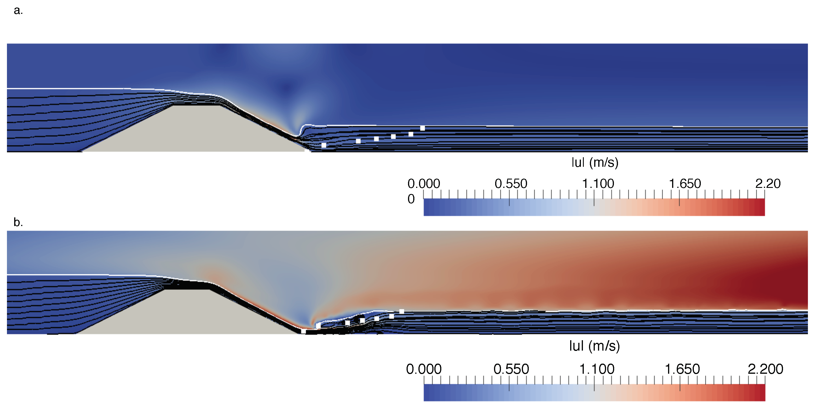
Figure 8.
Free surface features for submerged flow over an embankment weir without and with FSTD, the white dots denote the lower limit of the mixing layer presented in Fritz and Hager [5]: (a) without FSTD, (b) with FSTD.
Figure 8.
Free surface features for submerged flow over an embankment weir without and with FSTD, the white dots denote the lower limit of the mixing layer presented in Fritz and Hager [5]: (a) without FSTD, (b) with FSTD.

Figure 9.
Eddy-viscosity contours for submerged flow over an embankment weir: (a) without FSTD, high values of eddy viscosity around the free surface both in air and water phases, (b) with FSTD, the reduction in eddy viscosity around the free surface is clearly seen.
Figure 9.
Eddy-viscosity contours for submerged flow over an embankment weir: (a) without FSTD, high values of eddy viscosity around the free surface both in air and water phases, (b) with FSTD, the reduction in eddy viscosity around the free surface is clearly seen.

Figure 10.
Grid convergence study with FSTD for the numerical free surface elevation for flow around a pair of bridge piers: (a) along the center line through a pier m, (b) along the center of the channel m.
Figure 10.
Grid convergence study with FSTD for the numerical free surface elevation for flow around a pair of bridge piers: (a) along the center line through a pier m, (b) along the center of the channel m.

Figure 11.
Comparison of the experimental data [40] and the numerical results for the free surface elevation with and without FSTD: (a) along the center line through a pier m, (b) along the center of the channel m.
Figure 11.
Comparison of the experimental data [40] and the numerical results for the free surface elevation with and without FSTD: (a) along the center line through a pier m, (b) along the center of the channel m.

Figure 12.
Horizontal velocity (u) profiles over the water depth at various locations along the channel with and without FSTD: (a) m, (b) m, (c) m, (d) m.
Figure 12.
Horizontal velocity (u) profiles over the water depth at various locations along the channel with and without FSTD: (a) m, (b) m, (c) m, (d) m.

Figure 13.
Grid convergence study with FSTD for the free surface elevation in the case of flow over a broad-crested weir with a free stream outflow condition.
Figure 13.
Grid convergence study with FSTD for the free surface elevation in the case of flow over a broad-crested weir with a free stream outflow condition.

Figure 14.
Comparison of the experimental data [41] and the numerical results with and without FSTD for the free surface elevation over a broad-crested weir with free stream outflow condition.
Figure 14.
Comparison of the experimental data [41] and the numerical results with and without FSTD for the free surface elevation over a broad-crested weir with free stream outflow condition.

Figure 15.
Free surface features around the broad-crested weir with and without FSTD showing streamlines and velocity magnitude contours: (a) without FSTD, (b) with FSTD.
Figure 15.
Free surface features around the broad-crested weir with and without FSTD showing streamlines and velocity magnitude contours: (a) without FSTD, (b) with FSTD.

Figure 16.
Eddy viscosity around the broad-crested weir: (a) without FSTD, high values of eddy viscosity around the free surface in both air and water phases, (b) with FSTD, the reduction in the eddy viscosity around the free surface is clearly seen.
Figure 16.
Eddy viscosity around the broad-crested weir: (a) without FSTD, high values of eddy viscosity around the free surface in both air and water phases, (b) with FSTD, the reduction in the eddy viscosity around the free surface is clearly seen.

Figure 17.
Grid convergence study with FSTD for the free surface elevation in the case of plunging jet flow on an embankment weir.
Figure 17.
Grid convergence study with FSTD for the free surface elevation in the case of plunging jet flow on an embankment weir.

Figure 18.
Grid convergence study with FSTD for the horizontal velocity profiles over the water depth at various locations for plunging jet flow on an embankment weir: (a) m, (b) m, (c) m, (d) m.
Figure 18.
Grid convergence study with FSTD for the horizontal velocity profiles over the water depth at various locations for plunging jet flow on an embankment weir: (a) m, (b) m, (c) m, (d) m.

Figure 19.
Comparison of the experimental data [5] and the numerical results with and without FSTD for the free surface elevation in the case of plunging jet flow on an embankment weir.
Figure 19.
Comparison of the experimental data [5] and the numerical results with and without FSTD for the free surface elevation in the case of plunging jet flow on an embankment weir.

Figure 20.
Horizontal velocity (u) profiles over the water depth for plunging jet flow at various locations along the channel with and without FSTD (FSTD): (a) m, (b) m, (c) m, (d) m.
Figure 20.
Horizontal velocity (u) profiles over the water depth for plunging jet flow at various locations along the channel with and without FSTD (FSTD): (a) m, (b) m, (c) m, (d) m.

Figure 21.
Free surface features for plunging jet flow on an embankment weir without and with FSTD, the white dots denote the lower limit of the mixing layer presented in Fritz and Hager [5]: (a) without FSTD, (b) with FSTD.
Figure 21.
Free surface features for plunging jet flow on an embankment weir without and with FSTD, the white dots denote the lower limit of the mixing layer presented in Fritz and Hager [5]: (a) without FSTD, (b) with FSTD.

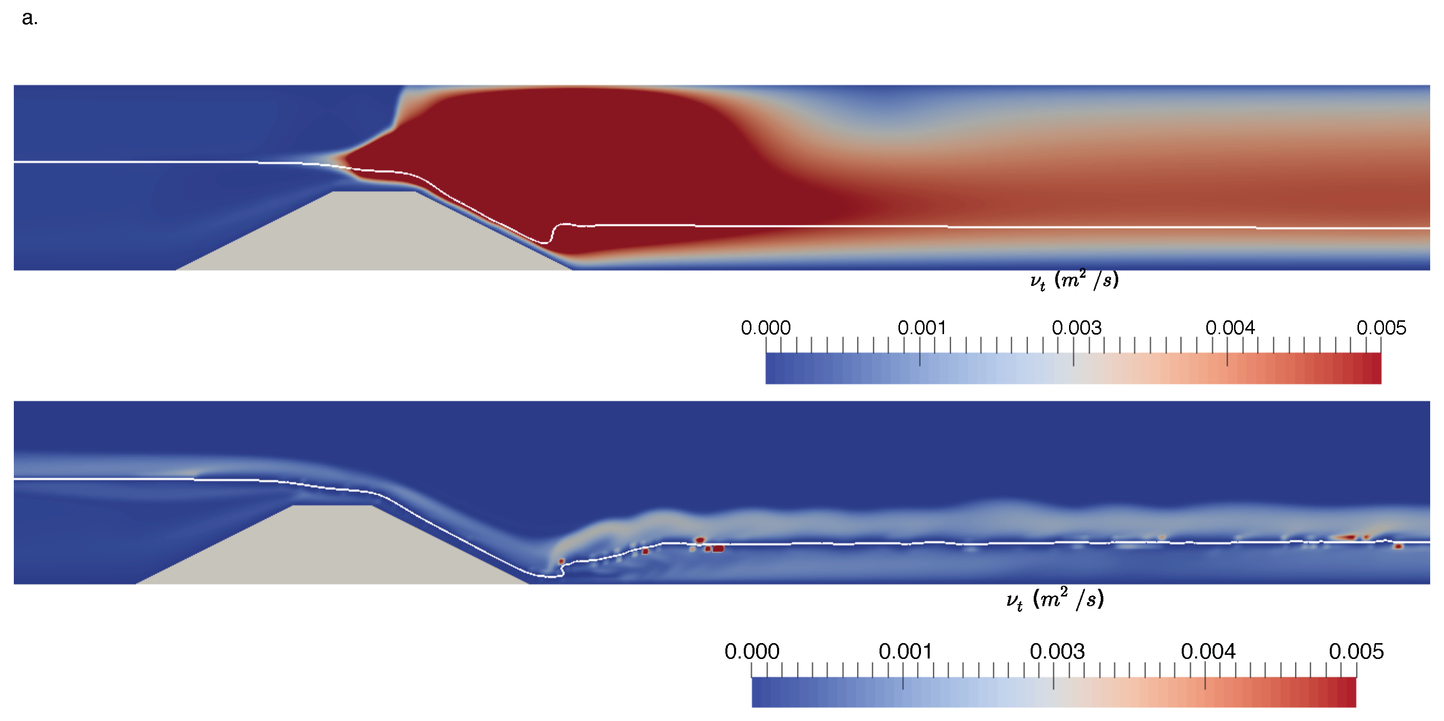
Figure 22.
Eddy-viscosity contours for plunging jet flow on an embankment weir: (a) without FSTD, high values of eddy viscosity are noticed around the interface in both air and water phases, (b) with FSTD, the reduction in the eddy viscosity around the free surface is clearly seen.
Figure 22.
Eddy-viscosity contours for plunging jet flow on an embankment weir: (a) without FSTD, high values of eddy viscosity are noticed around the interface in both air and water phases, (b) with FSTD, the reduction in the eddy viscosity around the free surface is clearly seen.

Figure 23.
Grid convergence study with FSTD for the free surface elevation in the case of free overflow on an embankment weir.
Figure 23.
Grid convergence study with FSTD for the free surface elevation in the case of free overflow on an embankment weir.

Figure 24.
Grid convergence study with FSTD for the horizontal velocity profiles over the water depth at various locations for free overflow on an embankment weir: (a) m, (b) m, (c) m, (d) m.
Figure 24.
Grid convergence study with FSTD for the horizontal velocity profiles over the water depth at various locations for free overflow on an embankment weir: (a) m, (b) m, (c) m, (d) m.

Figure 25.
Comparison of the experimental data [5] and the numerical results with and without FSTD for the free surface elevation in the case of free overflow on an embankment weir.
Figure 25.
Comparison of the experimental data [5] and the numerical results with and without FSTD for the free surface elevation in the case of free overflow on an embankment weir.

Figure 26.
Horizontal velocity (u) profiles over the water depth for free overflow on an embankment weir at various locations along the channel with and without FSTD: (a) m, (b) m, (c) m, (d) m.
Figure 26.
Horizontal velocity (u) profiles over the water depth for free overflow on an embankment weir at various locations along the channel with and without FSTD: (a) m, (b) m, (c) m, (d) m.

Figure 27.
Free surface features for free overflow on an embankment weir without and with FSTD, the white dots denote the lower limit of the mixing layer presented in Fritz and Hager [5]: (a) without FSTD, (b) with FSTD.
Figure 27.
Free surface features for free overflow on an embankment weir without and with FSTD, the white dots denote the lower limit of the mixing layer presented in Fritz and Hager [5]: (a) without FSTD, (b) with FSTD.

Figure 28.
Eddy-viscosity contours for free overflow on an embankment weir: (a) without FSTD, high values of eddy viscosity are noticed around the interface in both air and water phases, (b) with FSTD, the reduction in the eddy viscosity around the free surface is clearly seen.
Figure 28.
Eddy-viscosity contours for free overflow on an embankment weir: (a) without FSTD, high values of eddy viscosity are noticed around the interface in both air and water phases, (b) with FSTD, the reduction in the eddy viscosity around the free surface is clearly seen.

Figure 29.
Grid convergence study with FSTD for the numerical free surface elevation for flow around a pair of bridge piers: (a) along the center line through a pier m, (b) along the center of the channel m.
Figure 29.
Grid convergence study with FSTD for the numerical free surface elevation for flow around a pair of bridge piers: (a) along the center line through a pier m, (b) along the center of the channel m.

Figure 30.
Grid convergence study with FSTD for the horizontal velocity profiles over the water depth at various locations in the numerical channel: (a) m, (b) m, (c) m, (d) m.
Figure 30.
Grid convergence study with FSTD for the horizontal velocity profiles over the water depth at various locations in the numerical channel: (a) m, (b) m, (c) m, (d) m.

Figure 31.
Comparison of the experimental data [40] and the numerical results for the free surface elevation with and without FSTD: (a) along the center line through a pier m, (b) along the center of the channel m.
Figure 31.
Comparison of the experimental data [40] and the numerical results for the free surface elevation with and without FSTD: (a) along the center line through a pier m, (b) along the center of the channel m.

Figure 32.
Horizontal velocity (u) profiles over the water depth at various locations along the center of the channel in simulations with and without FSTD: (a) m, (b) m, (c) m, (d) m.
Figure 32.
Horizontal velocity (u) profiles over the water depth at various locations along the center of the channel in simulations with and without FSTD: (a) m, (b) m, (c) m, (d) m.

Figure 33.
Eddy viscosity along the center of the channel with bridge piers: (a) without FSTD, high values of eddy viscosity are seen around the free surface in both air and water phases, (b) with FSTD, reduction of the eddy viscosity around the interface is clearly seen.
Figure 33.
Eddy viscosity along the center of the channel with bridge piers: (a) without FSTD, high values of eddy viscosity are seen around the free surface in both air and water phases, (b) with FSTD, reduction of the eddy viscosity around the interface is clearly seen.

Figure 34.
Free surface features in the simulations with and without FSTD along with the velocity magnitude contours throughout the channel: (a) without FSTD, (b) with FSTD.
Figure 34.
Free surface features in the simulations with and without FSTD along with the velocity magnitude contours throughout the channel: (a) without FSTD, (b) with FSTD.


Table 1.
Overview of the flow conditions and cases investigated in the study.
| No. | Flow Condition | Case | Re | Fr |
|---|---|---|---|---|
| 1. | sub-critical flow | embankment weir | ||
| bridge piers | ||||
| 2. | sub-critical to super-critical flow | broad-crested weir | ||
| 3. | transitional flow | embankment weir | ||
| 4. | sub-critical to super-critical to sub-critical flow | embankment weir | ||
| bridge piers |
© 2019 by the authors. Licensee MDPI, Basel, Switzerland. This article is an open access article distributed under the terms and conditions of the Creative Commons Attribution (CC BY) license (http://creativecommons.org/licenses/by/4.0/).
Share and Cite
MDPI and ACS Style
Kamath, A.; Fleit, G.; Bihs, H. Investigation of Free Surface Turbulence Damping in RANS Simulations for Complex Free Surface Flows. Water 2019, 11, 456. https://doi.org/10.3390/w11030456
AMA Style
Kamath A, Fleit G, Bihs H. Investigation of Free Surface Turbulence Damping in RANS Simulations for Complex Free Surface Flows. Water. 2019; 11(3):456. https://doi.org/10.3390/w11030456
Chicago/Turabian StyleKamath, Arun, Gábor Fleit, and Hans Bihs. 2019. "Investigation of Free Surface Turbulence Damping in RANS Simulations for Complex Free Surface Flows" Water 11, no. 3: 456. https://doi.org/10.3390/w11030456
Note that from the first issue of 2016, this journal uses article numbers instead of page numbers. See further details here.