Combing Random Forest and Least Square Support Vector Regression for Improving Extreme Rainfall Downscaling

Abstract

A statistical downscaling approach for improving extreme rainfall simulation was proposed to predict the daily rainfalls at Shih-Men Reservoir catchment in northern Taiwan. The structure of the proposed downscaling approach is composed of two parts: the rainfall-state classification and the regression for rainfall-amount prediction. Predictors of classification and regression methods were selected from the large-scale climate variables of the NCEP reanalysis data based on statistical tests. The data during 1964–1999 and 2000–2013 were used for calibration and validation, respectively. Three classification methods, including linear discriminant analysis (LDA), random forest (RF), and support vector classification (SVC), were adopted for rainfall-state classification and their performances were compared. After rainfall-state classification, the least square support vector regression (LS-SVR) was used for rainfall-amount prediction for different rainfall states. Two rainfall states (i.e., dry day and wet day) and three rainfall states (dry day, non-extreme-rainfall day, and extreme-rainfall day) were defined and compared for judging their downscaling performances. The results show that RF outperforms LDA and SVC for rainfall-state classification. Using RF for three-rainfall-states classification and LS-SVR for rainfall-amount prediction can improve the extreme rainfall downscaling.

1. Introduction

Statistical precipitation downscaling is the process of making a link between a set of large-scale atmospheric variables (i.e., mean sea level pressure, vorticity, and geopotential height) and predictand (i.e., local precipitation). The large-scale predictors are essential for climate change research, but they do not actually provide a truthful presentation of the climate in a small basin. Generally, they have a spatial resolution coarser than 2 by 2 degrees in latitude and longitude, whereas hydrologists are more concerned with the catchment scale which is usually up to a few hundred square kilometers. This leads to a need for downscaling large-scale predictors to local precipitation. The NCEP reanalysis data set is a continually updated globally gridded data set that represents the state of the Earth’s atmosphere, incorporating observations and numerical weather prediction model output from 1948 to present. The NCEP reanalysis data is commonly used to develop a statistical relationship between large-scale climate factors with local rainfall for building (or training) downscaling models. The GCM outputs under climate change scenarios are then used as the inputs of downscaling models to project future precipitations for studying climate-change impacts [1]. The current study used the NCEP reanalysis data for building the proposed downscaling approach.

To date, there are many methods proposed for statistical downscaling using different techniques such as stochastic weather generators [2,3,4,5], weather typing method [6,7,8], resampling methods [9,10,11], and regression methods. The regression methods are attracting more attention and preferred to apply due to their flexibility and straightforwardness. There are numerous variant approaches of regression-based downscaling techniques such as logistic regression model [12], local polynomial regression [13], linear and non-linear regression [14], canonical correlation analysis [15], principal components [16], artificial neural network [17,18], support vector machine (SVM) [19,20,21,22], and beta regression [23].

Among these statistical downscaling methods, SVM shows its elegant and remarkable advantages comparing to the other methods. There are several studies which proved that SVM and variants of SVM are superior to ANN [19,24], multivariate analysis, and the Statistical DownScaling Model (SDSM) [24]. For instance, SVM performed better than ANN in predicting groundwater levels [25], runoff and sediment yield simulation [26], flood stage prediction [27], rainfall–runoff modeling [28], river flow forecasting [29,30], long-term discharge prediction [31], and modeling discharge-suspended sediment relationship [32]. SVM is also superior to multiple linear regression (MLR) in streamflow forecasting [33], autoregressive moving average (ARMA) in discharge prediction [31,34], autoregressive integrated moving average (ARIMA) in streamflow prediction [35], neural networks (NN), and MLR in daily water demand and inflow forecasting [36] and prediction of reservoir inflows [37]. In addition, SVM performed better than NN and empirical models in modeling daily reference evapotranspiration [38], neuro fuzzy inference system (ANFIS) in river flow forecasting [29] and daily forecasting of dam water levels [39], and genetic programming (GP) in forecasting monthly discharge time series [34].

However, many researches for downscaling precipitation at the catchment scale using SVM [19,24,40,41,42,43] conclude that the downscaling methods based on SVM performed well for normal rainfall but unsatisfactorily for extreme rainfall (i.e., underestimated extreme-rainfall amount). Tripathi et al. [19] detected that monthly precipitation downscaling by SVM could not reproduce the high rainfall observed in the historical records since the regression-based statistical downscaling models regularly cannot explain entire variance of the downscaled variable. They suggested that investigation of more large-scale predictor variables and a much longer validation period might likely provide more insight into this problem. A similar finding about the inability of SVM to mimic high rainfall has also been reported by Anandhi et al. [40].

In Taiwan, the downscaling methods based on SVM have been proposed by Chen et al. [24] and Yang et al. [41] for Shih-Men Reservoir catchment in northern Taiwan. The main structure of their proposed downscaling approach comprises the rainfall-state classification and the regression for rainfall amount. Chen et al. [24] used support vector classification (SVC) and linear discriminant analysis (LDA) for rainfall-state classification, while Yang et al. [41] only used LDA. Both the studies use the support vector regression (SVR) for the rainfall-amount prediction for wet days. Chen et al. [24] compared the performance of SVM to linear multiple regression and SDSM. The downscaled results showed that the SVM produced more accurate daily precipitation than SDSM and linear multiple regression. Yang et al. [41] found that the proposed downscaling model performed well in capturing the magnitude and variation of daily precipitations below 50 mm/day but underestimated the extreme rainfalls.

The aforementioned weakness of SVM in downscaling extreme rainfall inspires the current study to propose a modified statistical downscaling approach based on the methods developed by Chen et al. [24] and Yang et al. [41] for improving the extreme rainfall downscaling. The main structure of the proposed downscaling approach comprises the rainfall-state classification and the regression for rainfall-amount prediction. Three classification methods, including LDA, random forest (RF) and SVC, were adopted for rainfall-state classification and their performances were compared. The least square support vector regression (LS-SVR) was used for the rainfall-amount prediction for different rainfall states. Two rainfall states (i.e., dry day and wet day) and three rainfall states (dry day, non-extreme-rainfall day, and extreme-rainfall day) were defined and compared for judging their downscaling performances. Through the above comparisons, the optimal classification method with proper rainfall-state delineation can be found and linked with the rainfall-amount prediction method for improving the extreme rainfall downscaling.

The remaining part of this paper is organized as follows. Section 2 “Study Area and Data Set” provides a summary description of the study area and the data set including local rainfall and large-scale predictors. Section 3 “Methodology” describes three types of the proposed approach (i.e., Approach Type-I, Approach Type-II and Approach Type-III) and briefly introduces LDA, RF, and LS-SVR. Section 4 “Results and Discussion” describes the analysis results of rainfall-states classification and regression for rainfall-amount prediction by different classification methods and types of approach. Comparison of different classification methods (i.e., LDA, RF, and SVC) and different types of approach were made. Finally, Section 5 "Conclusions and Future Work” concludes the paper.

2. Study Area and Data Set

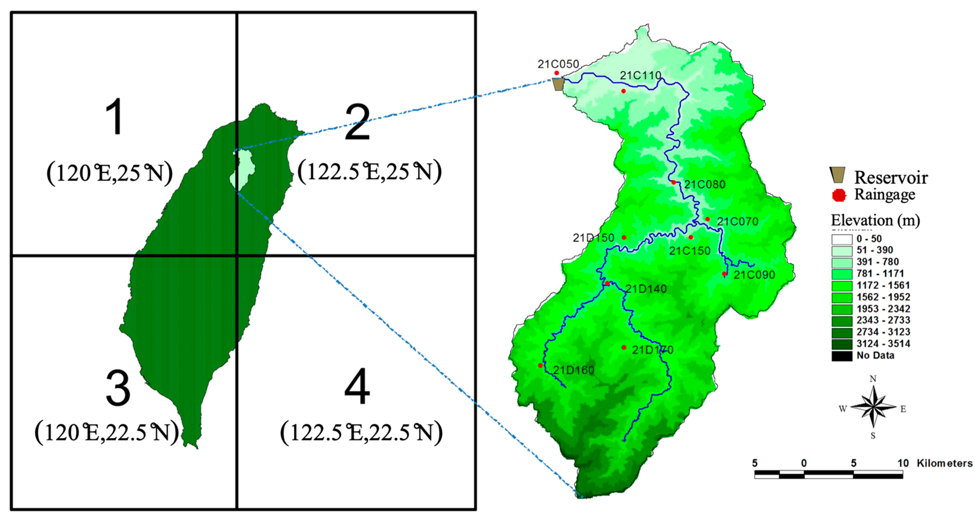
Shih-Men Reservoir, located in the Danshuei River basin in northern Taiwan, was completed in 1964 as a multifunction reservoir for water supply, agriculture, hydropower generation, and flood control. The Shih-Men Reservoir is a major reservoir with a storage capacity of around 3 × 10⁸ m³. Its upstream catchment (Figure 1) has an area of 763 km², and the basin ground elevation varies from 209 to 2609 meters. The average annual rainfall of the catchment is around 2250 mm.

Taiwan’s climate is governed by the East Asian Monsoon, which is divided into the summer and winter monsoons. Therefore, the Water Resources Bureau in Taiwan divided a year into the wet season (May–October) and the dry season (November–April) based on the summer and winter monsoons, respectively. The proportion of rainfall during the wet and dry seasons is about 7:3. The long-term daily rainfall from 1964 to 2013 at 10 rain gauges in the study area were collected to serve as the dataset (

Table 1. Information on rain gauges in Shih-Men reservoir catchment.

Station Name	Station Code	Location		Elevation (m)	Areal Weight
		Longitude (°E)	Latitude (°N)
Shih-Men	21C050	121.23	24.81	255	0.018
Ba-Ling	21C070	121.39	24.69	1220	0.075
Kao-Yi	21C080	121.35	24.71	620	0.127
Ka-La-Ho	21C090	121.39	24.64	1260	0.123
Chang-Hsing	21C110	121.30	24.80	350	0.151
San-Kuang	21C150	121.36	24.67	630	0.038
Hsiu-Luan	21D140	121.28	24.62	840	0.045
Yu-Feng	21D150	121.29	24.66	780	0.049
Hsin-Pai-Shih	21D160	121.25	24.59	1620	0.115
Chen-His-Pao	21D170	121.30	24.58	630	0.259

). The daily areal rainfalls in Shih-Men Reservoir catchment were calculated by using the Thiessen polygons method which determined the weights of all the stations listed in Table 1.

The daily data of 28 climate variables at the nearest grid point (i.e., Grid #2 at 122.5° E, 25° N in Figure 1) from 1964 to 2013 are obtained from the re-analysis data of National Centre for Environmental Prediction (NCEP)/National Centre for Atmospheric Research (NCAR) as listed in

Table 2. Large-scale climate factor (from NCEP).

No.	Acronym	Predictor
1	Mslp	Mean sea level pressure
2	p5_z	Vorticity at 500 hPa height
3	p8_z	Vorticity at 850 hPa height
4	p300	300 hPa geopotential height
5	p500	500 hPa geopotential height
6	p850	850 hPa geopotential height
7	p_f	Near surface geostrophic airflow velocity
8	p_z	Near surface vorticity
9	r500	Relative humidity at 500 hPa height
10	r850	Relative humidity at 850 hPa height
11	rhum	Near surface relative humidity
12	shum500	500 hPa specific humidity
13	Temp	Near surface air temperature
14	uas	Zonal surface wind speed
15	ua_700	700 hPa zonal wind speed
16	ua_850	850 hPa zonal wind speed
17	pr_wtr	Precipitable water
18	lftx	Surface lifted index
19	prec	Precipitation total
20	dswrf	Surface downwelling shortwave flux in air
21	dlwrf	Surface downwelling long flux in air
22	vas	Meridional surface wind speed
23	ta_700	700 hPa temperature
24	ta_850	850 hPa temperature
25	ta_925	925 hPa temperature
26	va_925	925 hPa meridional wind speed
27	uswrf	Surface upwelling shortwave flux in air
28	ulwrf	Surface upwelling longwave flux in air

. These climate variables were used as the candidates of model predictors. The areal rainfalls and the NCEP reanalysis data during 1964–1999 (calibration period) and 2000–2013 (validation period) were used for building statistical downscaling models and for examining and comparing downscaling results, respectively.

3. Methods

3.1. Proposed Approach

The main structure of the proposed downscaling approach comprises rainfall-state classification and regression for rainfall-amount prediction. Three classification methods, including LDA, RF, and SVC, were adopted for rainfall-state classification and their performances were compared. The LS-SVR was used for the rainfall-amount prediction for different rainfall states. Two rainfall states (i.e., dry day and wet day) and three rainfall states (i.e., dry day, non-extreme-rainfall day, and extreme-rainfall day) were defined and compared for judging their downscaling performances. Three types of approach were constructed and described as follows.

3.1.1. Approach Type-I

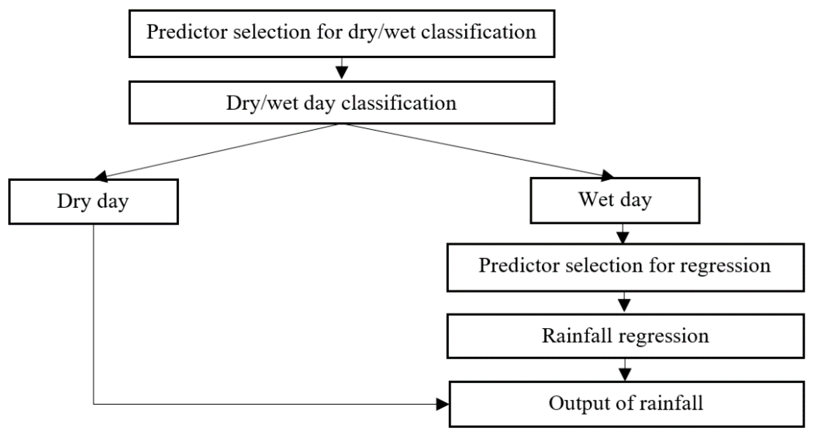
Two rainfall states (i.e., dry day and wet day) are defined for rainfall-state classification by using LDA, RF and SVC. The classification performances of LDA, RF, and SVC are compared to decide the best classification method for linking to the rainfall-amount prediction method. The LS-SVR is used for rainfall-amount prediction for the rainfall state of "wet day". The flowchart of Approach Type-I is shown in Figure 2. Dry day and wet day are defined as rainfall = 0 mm/day and rainfall > 0 mm/day, respectively. Previous researches used the SVC and LDA [24] and only LDA [41] for rainfall-state classification and the SVR for rainfall-amount prediction for the rainfall state “wet day”.

3.1.2. Approach Type-II

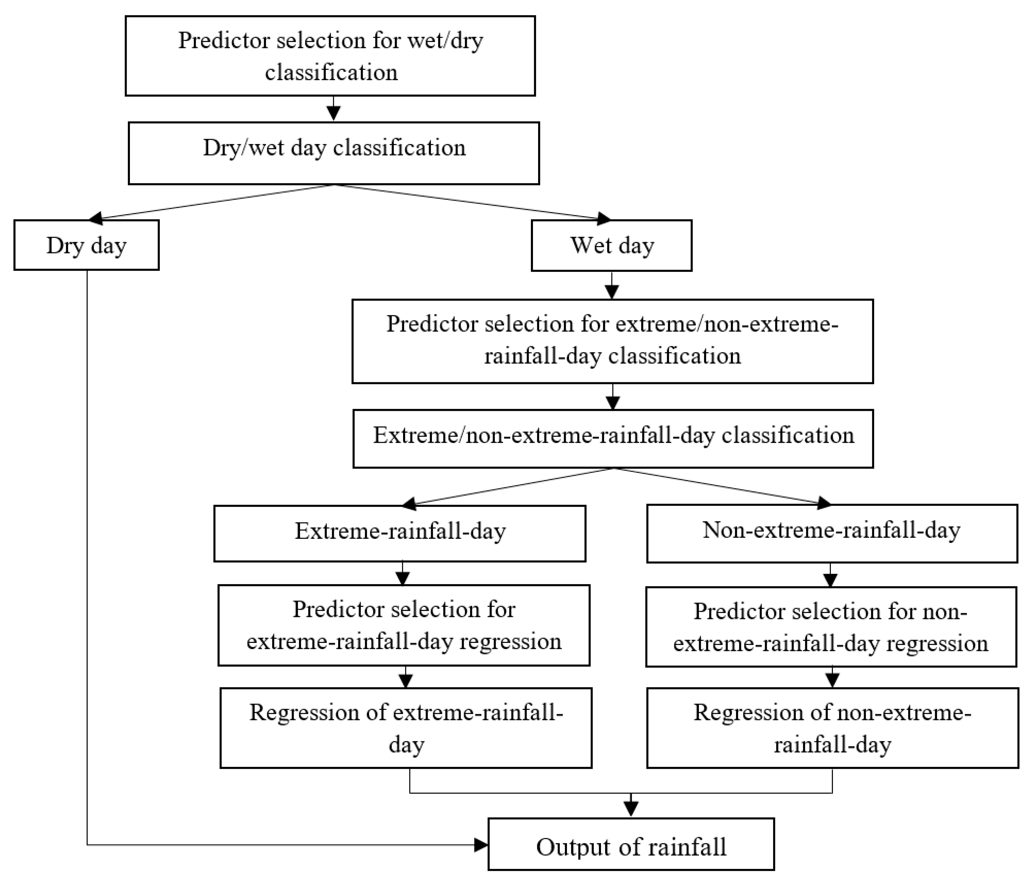
Two-steps classification is used for this type. The first step defines two rainfall states (dry day and wet day) and uses LDA, RF, and SVC for rainfall-state classification. For the second step, the rainfall state of “wet day” is further divided into two states “non-extreme-rainfall day” and “extreme-rainfall day” and the LDA, RF and SVC are also used for rainfall-state classification and compared to judge their performances. Non-extreme-rainfall day and extreme-rainfall day are defined as rainfall < 50 mm/day and rainfall ≥ 50 mm/day, respectively. The threshold of 50 mm/day is defined by the Central Weather Bureau of Taiwan, which is based on the historical cases for catchments where occurred torrents, landside, or rockfall with a rainfall greater than the threshold. After rainfall-state classification by the best classification method, the LS-SVR is used for rainfall-amount prediction for the rainfall states of “non-extreme-rainfall day” and “extreme-rainfall day”. The flowchart of Approach Type-II is shown in Figure 3.

3.1.3. Approach Type-III

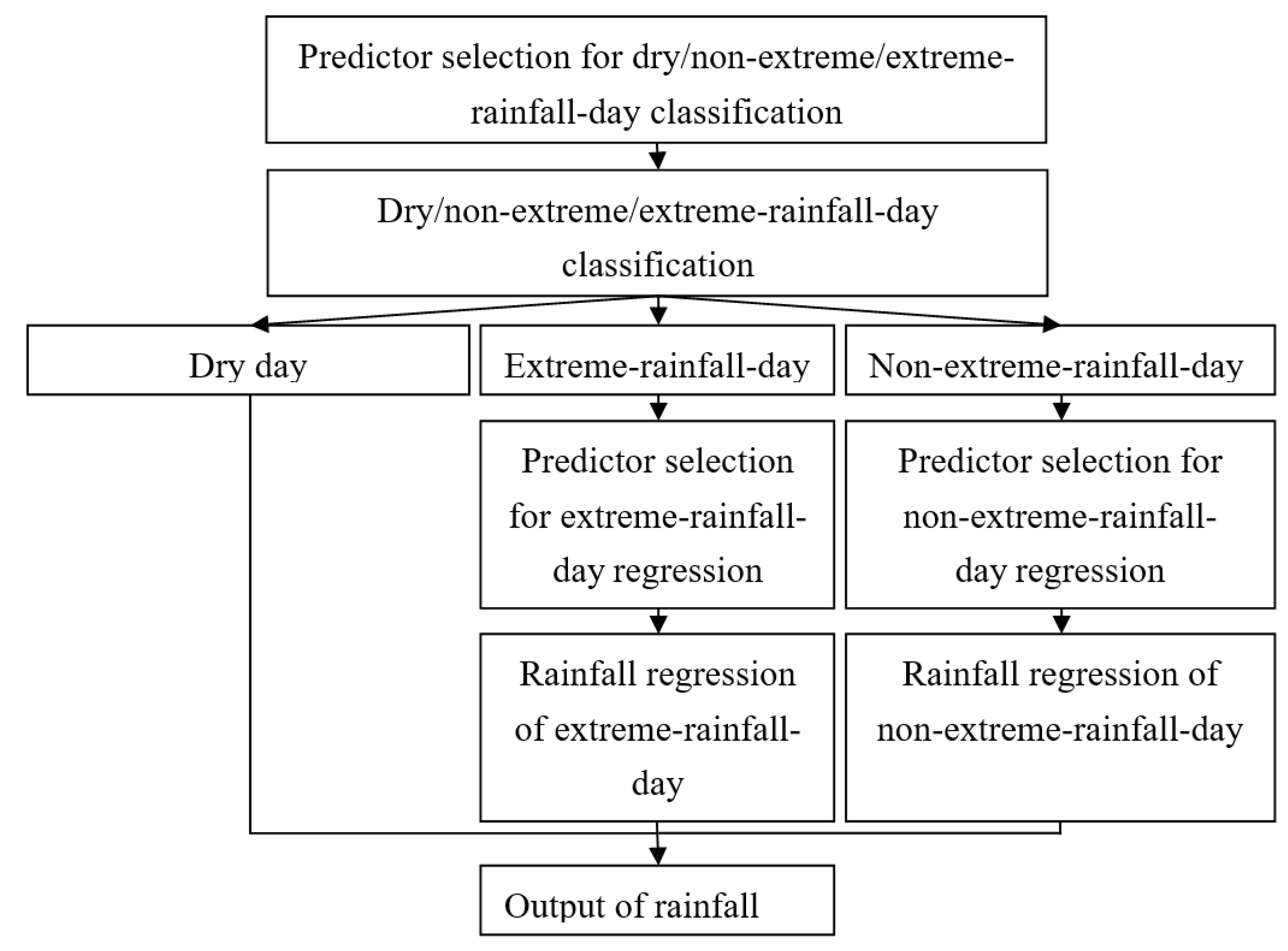
One-step classification for three rainfall states (dry day, non-extreme-rainfall day, and extreme-rainfall day) is used for this type, which means a day is directly classified into one of the three rainfall states. Three rainfall states are defined as Approach Type II and LDA, RF, and SVC are used for rainfall-state classification and compared to judge their performances. Coupled with the best classification method, the LS-SVR is used for rainfall-amount prediction for the rainfall states of “non-extreme-rainfall day” and “extreme-rainfall day”. The flowchart of Approach Type-III is shown in Figure 4.

The above three types of approach (i.e., Approach Type-I, Approach Type-II, and Approach Type-III) are used for daily rainfall downscaling and their performances are compared. Through the comparisons, the optimal classification method with proper rainfall-state delineation can be found and linked with the rainfall-amount prediction method for improving the extreme rainfall downscaling.

3.2. Linear Discriminant Analysis

LDA, originally developed by Fisher (1936) [44], finds a linear discriminant function L to determine the class of a predictand based on a set of n predictors (x₁, x₂,…, x_n).

$$L=a_0+a_1{x}_1+a_2{x}_2+\dots +a_n{x}_n$$

(1)

The parameters (a₀, a₁, a₂,…, a_n) are calibrated from the training data of predictors and a predefined class label (for example, +1 and −1) of the predictand. The linear discriminant function L is then used to predict the class of a new predictand according to the estimated class label. In the current study, LDA was performed by the “fitcdiscr” function provided by MathWorks.

3.3. Random Forest

Random forests (RFs) are very flexible and powerful ensemble classifiers based on decision trees which were firstly developed by Breiman (2001) [45,46,47]. Very recently, there has been increasing interest in RF and it was applied in different areas to solve classification problems [48,49,50,51]. However, there are few applications of RFs to classify rainfall states. The only such application of RFs was recently proposed to predict rainfall occurrence in Besut station, on the east coast of Peninsular Malaysia [52]. RFs have two calibration parameters which consist of the number of variables (mtry) and the number of trees (ntree). In the present study, the value of mtry which equal the square of number of features were implemented for each classification model. Such value can generally give near optimum results for classification tasks [53]. The value of ntree ranging from 0 to 2000 was used for searching the optimal value (ntree = 500) adopted in this work. The randomForest package [54] is used in this study.

3.4. Least Square-Support Vector Machine

The least squares support vector machine (LS-SVM) algorithm is an improved algorithm of standard SVM, which provides a computational advantage (reduces the computational burden) over standard SVM by converting quadratic optimization problem into a system of linear equations [55]. In the LS-SVM algorithm, a solution is obtained by solving a linear set of equations instead of solving a quadratic programming problem involving standard SVM. The LS-SVM can be used for both classification and regression problems. In the current study, the LS-SVR is used for constructing rainfall state classification and the daily rainfall downscaling models. The description of SVC for rainfall states classification can be found in more detail in Chen et al. [24]. The brief description on the LS-SVR is as follows.

By considering inputs x_i (predictors: climate variables) and output y_i (predictand: local rainfall). According to the LS-SVR method, the nonlinear LS-SVR function can be expressed as

$$f(x)=w^T\phi (x)+b$$

(2)

where f indicates the relationship between the climate variables (predictors) and local rainfall (predictand), w, $\phi$ and b are the m-dimensional weight vector, mapping function and bias term, respectively [56].

Using the function estimation error, the regression problem can be expressed regarding structural minimization principle as

$$\min J(w,e)=\frac{1}{2}{w}^{T}w+\frac{\gamma }{2}{\displaystyle \sum _{i=1}^m{e}_i^2}$$

(3)

which is subjected to the following constraints:

$$y_i=w^T\phi (x_i)+b+e_i\left(i=1,2,\dots ,m\right)$$

(4)

where $\gamma$ refers the penalty term and e_i is the training error for x_i.

To find the solutions of w and e, the Lagrange multiplier optimal programming method is employed to solve Equation (3). The objective function can be determined by altering the constraint problem into an unconstraint problem. The Lagrange function L can be expressed as

$$L(w,b,e,\alpha )=J(w,e)-{\displaystyle \sum _{i=1}^m{\alpha }_i}\{w^T\phi (x_i)+b+e_i-y_i\}$$

(5)

where ${\alpha }_i$ are the Lagrange multipliers.

Taking into account the Karush–Kuhn–Tucker (KKT) conditions [56], the optimal conditions can be obtained by taking the partial derivatives of Equation (5) with respect to w, b, e and α, respectively as

$$\{\begin{array}{l}w={\displaystyle \sum _{i=1}^m{\alpha }_i\phi (x_i)}\\ {\displaystyle \sum _{i=1}^m{\alpha }_i=0}\\ {\alpha }_i=\gamma e_i\\ w^T\phi (x_i)+b+e_i-y_i=0\end{array}$$

(6)

Thus, the linear equations can be derived after elimination of e_i and w as

$$\left[\begin{array}{l}0-Y^T\\ YZ{Z}^T+I/\gamma \end{array}\right]\left[\begin{array}{l}b\\ \alpha \end{array}\right]=\left[\begin{array}{l}0\\ 1\end{array}\right]$$

(7)

where $Y=(y_1,\dots ,y_m),Z=(\phi {(x_1)}^T{y}_1,\dots ,\phi {(x_m)}^T{y}_m),I=(1,\dots ,1),\alpha =({\alpha }_1,\dots ,{\alpha }_l)$

By defining kernel function $K(x,x_i)=\phi {(x)}^T\phi (x_i),i=1,\dots ,m$, which is satisfied with Mercer’s condition (the readers could refer to the paper of Suykens et al. [57] to get more explanation of Mercer’s condition). As a result, the LS-SVR can be represented as

$$f(x)={\displaystyle \sum _{i=1}^m{\alpha }_{i}K(x,x_i)+b}$$

(8)

In this study, the commonly used RBF kernel function given in Equation (9) was used.

$$K(x,x_i)=\exp (-||x-x_i|{|}^2/2{\sigma }^2)$$

(9)

Before calibrating the LS-SVR, the values of local rainfall and predictor variables were normalized by their respective means and standard deviations. The normalized values of local rainfall and predictor variables were then utilized for calibrating the LS-SVR. The LS-SVR needs the calibration of two parameters: the penalty term (γ) and the kernel width (σ). In the training period of LS-SVR, the grid-search method [58] is used to estimate optimal parameters. The grid search method can yield an optimal parameter set and employing a cross-validation procedure can prevent the downscaling model from over-fitting. In the current study, the LS-SVR was performed by the package provided by MATLAB toolbox (http://www.esat.kuleuven.ac.be/sista/lssvmlab).

4. Results and Discussion

4.1. Rainfall-State Classification

For Approach Type-I, the calibration data (including the NCEP reanalysis data and local rainfalls) were separated into two groups (i.e., wet-day group and dry-day groups) according to daily local rainfalls in both dry and wet seasons. The two-sample Kolmogorov–Smirnov test was then performed to choose suitable predictors of the NCEP reanalysis data. This study used the two-sample Kolmogorov–Smirnov test to select predictors of the NCEP reanalysis data that are distinguishable between the dry-day group and the wet-day group. The predictors which showed a significant difference between two groups (with a significance level of 0.01) were considered as the suitable predictors for classification models. In the current study, the test was performed by the “kstest2” function provided by MathWorks. The selected predictors after testing are mean sea level pressure (mslp), vorticity (p_z, p5_z, and p8_z), geopotential height (p300, p500, and p850), relative humidity (r500, r850, and rhum), zonal wind speed (ua_700 and ua_850), meridional wind speed (vas and va_925), and temperature (ta_700, ta_850, and ta_925). The above selected predictors for Approach Type-I were also used for Approach Type-II and Approach Type-III.

For Approach Type-II, after conducting the same aforementioned process of Approach Type-I, the given wet days were further classified into non-extreme-rainfall-day group and extreme-rainfall-day group. For Approach Type-III, the calibration data (including the NCEP reanalysis data and local rainfalls) were separated into dry-day, non-extreme-rainfall-day, and extreme-rainfall-day groups according to the daily local rainfalls. Because there are only few extreme rainfalls during the dry season, the classification of non-extreme-day and extreme-day was only conducted during the wet season.

The accuracies of (1) the dry-day/wet-day classification for Approach Type-I, (2) the non-extreme-rainfall-day/extreme-rainfall-day classification for Approach Type-II and (3) the dry-day/non-extreme-rainfall-day/extreme-rainfall-day classification for Approach Type-III can be estimated respectively as

$$Accuracy(wet/dry)=\frac{D|D+W|W}{D+W}$$

(10)

$$Accuracy(non-extreme/extreme)=\frac{N|N+E|E}{N+E}$$

(11)

$$Accuracy(dry/non-extreme/extreme)=\frac{D|D+N|N+E|E}{D+N+E}$$

(12)

where D is the number of dry days, W is the number of wet days, D|D indicates the number of days that a dry day is correctly classified as a dry day, W|W indicates the number of wet days that a wet day correctly classified as a wet day, N is the number of non-extreme-rainfall days, E is the number of extreme-rainfall days, N|N indicates the number of days that a non-extreme-rainfall day is correctly classified as a non-extreme-rainfall day, and E|E indicates the number of extreme-rainfall days that an extreme-rainfall day correctly classified as an extreme-rainfall day.

Since the formulas for calculating the classification accuracies for Approach Type-I (Equation (10)), Approach Type-II (Equations (10) and (11)) and Approach Type-III (Equation (12)) are different, the results in

Table 3. Classification accuracy (%) of dry/wet day and extreme-rainfall/non-extreme-rainfall day.

Type of Approach	LDA		RF		SVC
	Wet Season	Dry Season	Wet Season	Dry Season	Wet Season	Dry Season
Type-I	75.38	75.39	79.35	75.64	74.00	72.42
Type-II Step 1 1	75.38	75.39	79.35	75.64	74.00	72.42
Type-II Step 2	95.26	97.62	95.31	98.33	93.06	96.83
Type-III	66.72	68.85	74.46	69.71	69.44	68.63

¹ Note: Step 1 in Approach Type-II is similar to Approach Type-I. LDA: linear discriminant analysis; RF: random forest; SVC: support vector classification.

were only used for comparing the classification performances by different methods (LDA, SVC, and RF) in each approach, not for judging which type of approach is the best in the classification step.

The performances of (1) the dry-day/wet-day classification for Approach Type-I, (2) the non-extreme-rainfall-day/extreme-rainfall-day classification for Approach Type-II and (3) the dry-day/non-extreme-rainfall-day/extreme-rainfall-day classification for Approach Type-III are shown in Table 3. There are three methods (i.e., LDA, RF, and SVC) which were used for classifying rainfall states in both wet and dry season. The accuracies of dry-day/wet-day classification are generally higher than 72%. The performance of the dry-day/wet-day classification models in the wet season are better than those in the dry season for all three methods. The accuracies of dry-day/non-extreme-rainfall-day/extreme-rainfall-day classification are generally higher than 66%. The accuracies of non-extreme-rainfall-day/extreme-rainfall-day classification in Step 2 of Approach Type-II are generally higher than 93%.

The proportions of individual states (dry day, non-extreme-rainfall day, and extreme-rainfall day) during the wet season in the calibration period are 33.83%, 62.72%, and 3.45%, respectively. In the validation period, the proportions of individual states (dry day, non-extreme-rainfall day, and extreme-rainfall day) during the wet season are 34.07%, 61.54%, and 4.39%, respectively. Improvement of extreme rainfall downscaling is the main concern of the current study. For emphasizing the classification accuracy for extreme-rainfall-day state, the classification accuracies (%) of extreme-rainfall day during wet season were presented in

Table 4. Classification accuracy (%) of extreme-rainfall-day state during the wet season.

Type of Approach	LDA	RF	SVC
Type-II Step 2	49.52	56.19	30.48
Type-III	47.36	47.57	15.53

. The dry season was not taken into account because most of extreme-rainfall-day occurred during wet season.

By comparing the performances of the three classification methods, it is found that RF outperforms LDA and SVC by the largest classification accuracy (%) of dry/wet day and extreme-rainfall/non-extreme-rainfall day in Table 3, and the largest classification accuracy of extreme-rainfall-day state during the wet season in Table 4. Therefore, the outputs of RF classification models were selected as inputs for the regression models to simulate rainfall amounts.

4.2. Regression for Rainfall-Amount

Before establishing the regression models, the principal component analysis (PCA) was used to transform the predictors (i.e., the 28 climate variables of the NCEP reanalysis data) to new matrices as the input matrices for LS-SVR models. The purposes of PCA are to eliminate the multicollinearity and reduce the dimension of a large data set. In the current study, PCA was carried out with the NCEP reanalysis data obtained from the nearest grid point of the study area. Nine principal components were selected based on the eigen-values which are greater than 1.0, which can explain more than 85% of the variance of the data set (i.e., the NCEP reanalysis data). The transformed variables by the nine principal components were used as the predictors of the LS-SVR models for different types of approach. Based on the transformed variables by PCA, the LS-SVR models were developed for the wet and dry seasons separately. PCA reduced the dimension of the large data set from a sample size of 143,080 corresponding to 28 predictors to a smaller sample size of 45,990 corresponding to nine principle components, which considerably reduces the computational consumption. The local rainfall and the NCEP reanalysis data during the calibration period were used to tune the two hyper-parameters of each LS-SVR model.

Table 5. The tuned parameters of least square support vector regression (LS-SVR) models.

Season	Model	Penalty Term	Kernel Width
Wet	Approach Type-I for wet day	4.62	6.27
Wet	Approach Type-II for non-extreme-rainfall day	1.64	5.95
Wet	Approach Type-II for extreme-rainfall day	78.50	1.12
Wet	Approach Type-III for non-extreme-rainfall day	2.32	5.40
Wet	Approach Type-III for extreme-rainfall day	73.65	1.05
Dry	Approach Type-I for wet day	10.89	32.60
Dry	Approach Type-II for wet day	11.14	31.23
Dry	Approach Type-III for wet day	24.34	52.81

lists the tuned parameters of the LS-SVR models. Since most of extreme rainfalls occur during the wet season, the observed data were separated into two groups (i.e., non-extreme-rainfall group and extreme-rainfall group) for Approach Type-II and Approach Type-III. As there are too few extreme rainfalls during the dry season, only Approach Type-I approach was used for this season. The rainfalls calculated by the LS-SVR models are normalized values which should be converted to their original scale.

The data of 1964–1999 were used to train the classification and regression models. During the validation period (2000–2013), the 2990 wet days were extracted for construction and evaluation of the LS-SVR models. In order to demonstrate the accuracy of the proposed approach objectively and evidently, three statistical measures (i.e., Mean, standard deviation (SD) and Skewness) are employed for examining whether the downscaling rainfalls by the proposed approach conserves the statistical characteristics of the observed rainfalls.

Table 6. Statistics of regression results on wet days in the calibration period.

Statistics	Approach Type-I	Approach Type-II	Approach Type-III	Observation
Mean (mm)	10.36	10.33	10.33	10.29
SD (mm)	21.49	24.15	24.12	26.87
Skewness (mm)	10.52	10.22	10.32	9.52

and

Table 7. Statistics of regression results on wet days during the validation period.

Statistics	Approach Type-I	Approach Type-II	Approach Type-III	Observation
Mean (mm)	10.52	11.51	10.57	12.29
SD (mm)	22.55	30.21	28.50	34.94
Skewness (mm)	9.12	8.05	9.09	8.08

list these above measures for comparing the performances of the three types of approach. From the tables, the output of Approach Type-II is slightly better than that of Approach Type-III. The simulated values of Mean, SD, and skewness in Approach Type-II are closer to the observed values than those in Approach Type-III except for SD during the calibration period (Table 6). In general, the Mean and SD of simulated rainfalls from the three types of approach tend to underestimate the observed rainfalls. However, Approach Type-II and Approach Type-III conserve the Mean and SD of observed rainfalls significantly more than Approach Type-I.

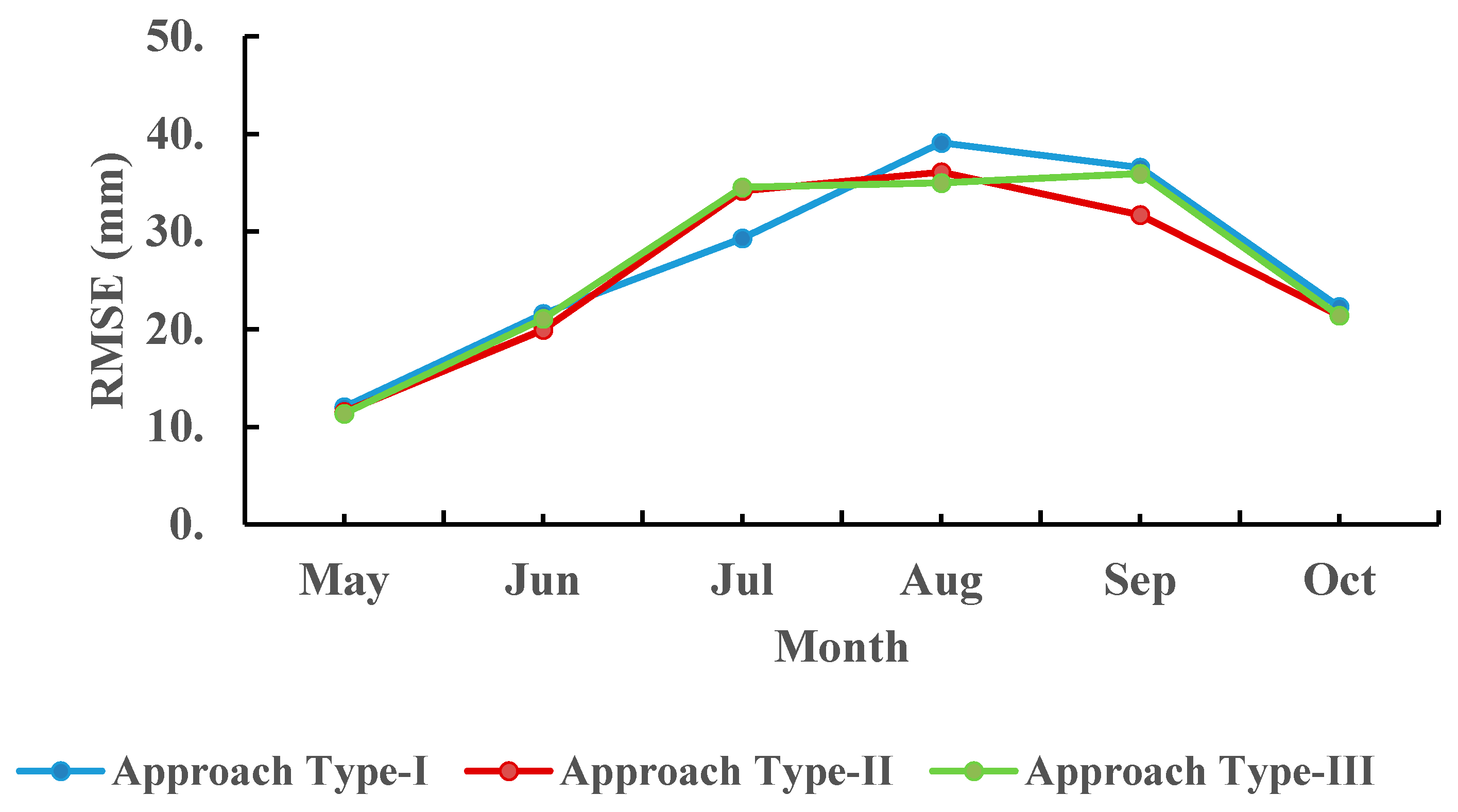
To compare the simulated performances for each type of approach, Figure 5 shows the RMSE of individual months for three types of approach during the wet season in the validation period. Since most of extreme rainfalls occur during the wet season and the efficiency of Approach Type-II and Approach Type-III strongly represents during this season, only the RMSE of individual months during the wet season is presented in the figure. In Figure 5, Approach Type-III and Approach Type-II have the RMSE smaller than that of Approach Type-I in most of months except for the month of July. This is because that the classification models of Approach Type-II and Approach Type-III only have the accuracy around 50% (correctly classified 9 extreme rainfalls in a total of 18 extreme rainfalls) in July. While the accuracy in August and September are 64.29% and 79.16%, respectively, for Approach Type-III, which is much better than Approach Type-I. This implies that the accuracy of extreme rainfall classification has a significant impact on the efficiency of the proposed approach. The classification of the non-extreme-day/extreme-day showed that the performance in August and September are better when compared to July, which might be attributed to the number of heavy rainfalls in August and September.

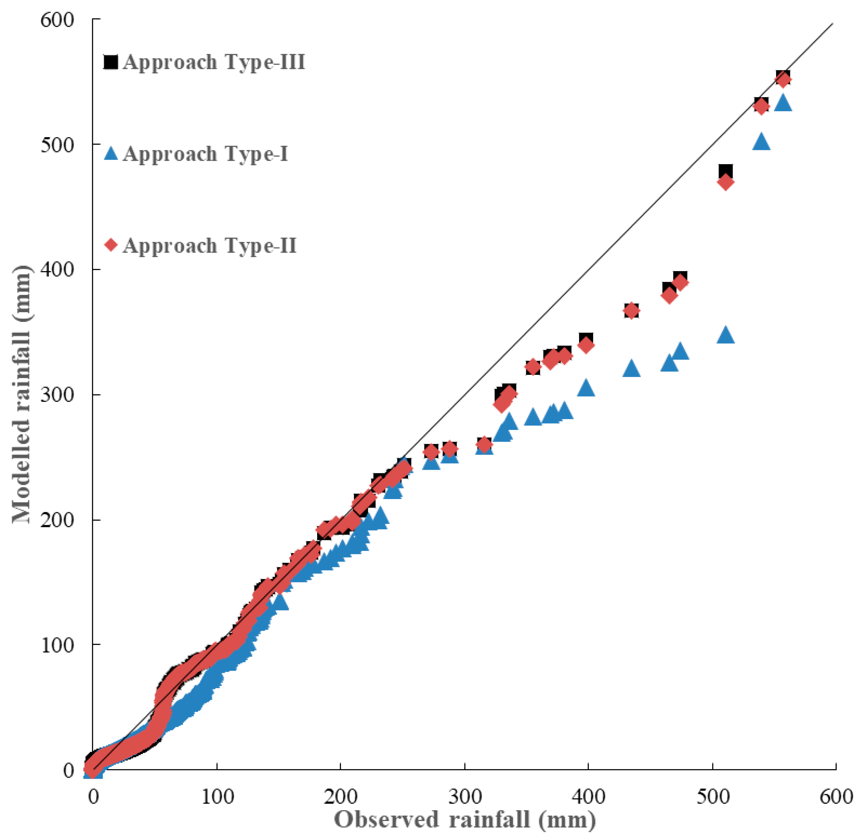
In general, Approach Type-II and Approach Type-III show that their performances in terms of Mean, SD, and skewness are better than the performance of Approach Type-I. Approach Type-II shows its SD significantly better than that of Approach Type-I and Approach Type-III. Approach Type-II is slightly better than Approach Type-III in terms of Mean and skewness. It is apparent that both Approach Type-II and Approach Type-III outperform Approach Type-I in term of generation of extreme rainfalls during both calibration and validation periods (Figure 6 and Figure 7). Approach Type-II and Approach Type-III are quite similar in reproducing extreme rainfalls.

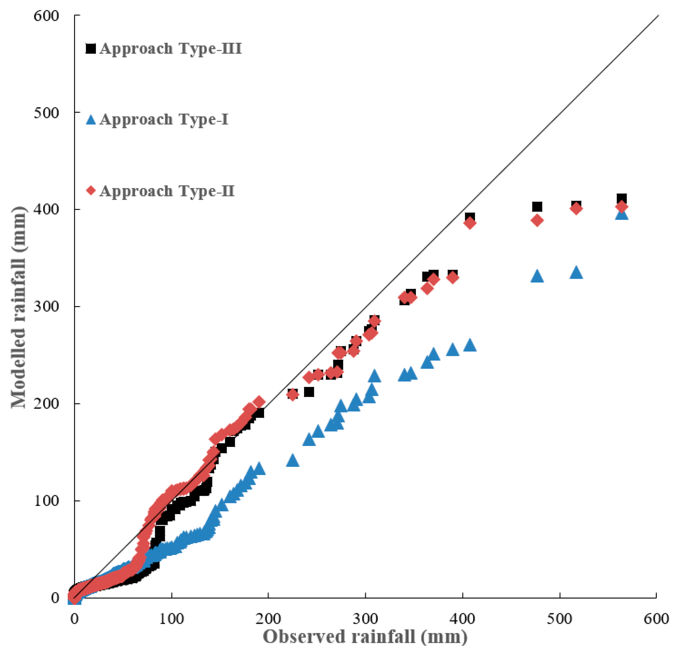
Figure 6 and Figure 7 shows the daily downscaling rainfalls for the three types of approach in the form of quantile–quantile (Q–Q) plots. It reveals that Approach Type-II and Approach Type-III significantly outperform the Approach Type-I when rainfalls are larger than around 50 mm/day. This results are consistent with the comparison results of statistical characteristics for both Approach Type-II and Approach Type-III with a better skewness estimate than that of Approach Type-I. Overall, both Approach Type-II and Approach Type-III models perform better than Approach Type-I in downscaling extreme rainfall amounts. It is worth noting that there are three very extreme rainfalls greater than 450 mm/day during the validation period (Figure 7) and the three very extreme rainfalls were still significantly underestimated. This is because there are too few data of very extreme rainfalls for training the models.

4.3. Discussion

Negative output values from the LS-SVR models were set to zero in the current study. The proportion of negative values among the total number of wet days are 3.59% in Approach Type-I, 1.45% in Approach Type-II, and 1.96% in Approach Type-III during the calibration period. Those are 3.89% in Approach Type-I, 2.68% in Approach Type-II, and 3.65 in Approach Type-III during the validation period. It is obvious that Approach Type-II and Approach Type-III have less negative output values than Approach Type-I. Separation of wet days into non-extreme-rainfall-day and extreme-rainfall-day data groups can get the benefit in terms of gaining less negative output values from LS-SVR models. The reason might be that the separation supports the LS-SVR models in Approach Type-II and Approach Type-III to gain more suitable parameters for each data groups (i.e., non-extreme-rainfall day and extreme-rainfall day), while the LS-SVR model in Approach Type-I only tunes one set of parameters for only a wet-day data group.

The poor skill of downscaling in capturing extreme events is attributed to two reasons. First, the standardization may reduce the bias in the mean and variance of the predictor variable, but it is much harder to accommodate the bias in large-scale patterns of atmospheric circulation or unrealistic intervariable relationships between predictor variables. The other reason may be that the NCEP reanalysis data are not able to reproduce the extreme value as many extreme events occur at a much smaller scale.

Even though the poor skill of GCM downscaling in capturing extreme events, it is found that the proposed downscaling approach with three rainfall states classification (i.e., Approach Type-II and Approach Type-III) can improve the extreme-rainfall downscaling by Approach Type-I. These two types of approach (i.e., Approach Type-II and Approach Type-III) can conserve the statistical characteristics (e.g., standard deviation and skewness) of observation data, which is a big challenge of many downscaling models. It is noted that Approach Type-II and Approach Type-III performed the extreme-rainfall downscaling better than Approach Type-I during the wet season.

5. Conclusions and Future Work

The current study proposes a statistical downscaling approach for improving daily extreme rainfall simulation at Shih-Men Reservoir catchment in northern Taiwan, which comprises rainfall-state classification and regression for rainfall-amount prediction. Three classification methods (i.e., LDA, RF, and SVC) were adopted for rainfall-state classification and the LS-SVR was used for the rainfall-amount prediction for different rainfall states. Two rainfall states (i.e., dry day and wet day) and three rainfall states (dry day, non-extreme-rainfall day, and extreme-rainfall day) were defined and compared for judging their downscaling performances.

Three types of approach (i.e., Approach Type-I, Approach Type-II and Approach Type-III) have been developed and tested for rainfall downscaling in the study area. Approach Type-I adopts two rainfall states for rainfall-state classification. Approach Type-II and Approach Type-III adopt three rainfall states for two-steps and one-step rainfall-state classification, respectively. The results reveal that RF outperforms LDA and SVC for the rainfall-state classification for all three types of approach. Approach Type-II and Approach Type-III, which use RF for three-rainfall-states classification and LS-SVR for rainfall-amount prediction, have better extreme rainfall simulation than Approach Type I. Future work can apply the two types of approach for the areas with more extreme-rainfall data to validate the performances for extreme-rainfall downscaling.

Adopting a proper threshold of daily extreme rainfall is essential for extreme/non-extreme-rainfall-day classification. The threshold of extreme rainfall strongly influences the rainfall-state classification performance. The current study adopted 50 mm/day as the threshold of extreme rainfall which is defined by the Central Weather Bureau of Taiwan. Using the thresholds less than 50 mm/day (i.e., 30 mm/day and 10 mm/day) for getting more extreme events (i.e., larger sample size) was also tested and had no improvement for rainfall-state classification in the study case. Therefore, using an inappropriate threshold of extreme rainfall may result in a failure of extreme rainfall classification. Selection of a proper threshold of extreme rainfall should be further investigated scientifically and carefully. The future work may apply the detrended fluctuation analysis (DFA) to choose an appropriate threshold of extreme rainfall for a catchment [59].

The choice of a certain reanalysis dataset is often motivated by either ease of access (availability of the dataset at the institution), ease of use (availability of code to read it), or by the preference for the local provider [60]. In the current study, the NCEP reanalysis data were used for ease of access and ease of use. The other available reanalysis data (e.g., European Centre for Medium-Range Weather Forecasts, ECMWF) with a much better spatial resolution data can be the alternatives for future work.

References

- Arora, H.; Ojha, C.S.P.; Kashyap, D. Effect of Spatial Extent of Atmospheric Variables on Development of Statistical Downscaling Model for Monthly Precipitation in Yamuna-Hindon Interbasin, India. J. Hydrol. Eng. 2016, 21, 05016019. [Google Scholar] [CrossRef]
- Khalili, M.; Leconte, R.; Brissette, F. Stochastic multisite generation of daily precipitation data using spatial autocorrelation. J. Hydrometeorol. 2007, 8, 396–412. [Google Scholar] [CrossRef]
- Tung, C.P.; Haith, D.A. Global-warming effects on New York streamflows. J. Water Resour. Plan. Manag. 1995, 121, 216–225. [Google Scholar] [CrossRef]
- Hughes, J.P.; Guttorp, P. A class of stochastic models for relating synoptic atmospheric patterns to regional hydrologic phenomena. Water Resour. Res. 1994, 30, 1535–1546. [Google Scholar] [CrossRef]
- Yu, P.S.; Yang, T.C.; Wu, C.K. Impact of climate change on water resources in southern Taiwan. J. Hydrol. 2002, 260, 161–175. [Google Scholar] [CrossRef]
- Bardossy, A.; Plate, E.J. Space-time model for daily rainfall using atmospheric circulation patterns. Water Resour. Res. 1992, 28, 1247–1259. [Google Scholar] [CrossRef]
- Von Storch, H.; Zorita, E.; Cubasch, U. Downscaling of global climate change estimates to regional scales: An application to Iberian rainfall in wintertime. J. Clim. 1993, 6, 1161–1171. [Google Scholar] [CrossRef]
- Bárdossy, A. Disaggregation of daily precipitation. In Proceedings of the Workshop on Ribamod–River Basin Modelling, Management and Flood Mitigation Concerted Action, Padua, Italy, 25–26 September 1997. [Google Scholar]
- Buishand, T.A.; Brandsma, T. Multisite simulation of daily precipitation and temperature in the Rhine basin by nearest-neighbor resampling. Water Resour. Res. 2001, 37, 2761–2776. [Google Scholar] [CrossRef]
- Murphy, J. Predictions of climate change over Europe using statistical and dynamical downscaling techniques. Int. J. Climatol. 2000, 20, 489–501. [Google Scholar] [CrossRef] [Green Version]
- Palutikof, J.P.; Goodess, C.M.; Watkins, S.J.; Holt, T. Generating rainfall and temperature scenarios at multiple sites: Examples from the Mediterranean. J. Clim. 2002, 15, 3529–3548. [Google Scholar] [CrossRef]
- Abaurrea, J.; Asín, J. Forecasting local daily precipitation patterns in a climate change scenario. Clim. Res. 2005, 28, 183–197. [Google Scholar] [CrossRef] [Green Version]
- George, J.; Janaki, L.; Gomathy, J.P. Statistical downscaling using local polynomial regression for rainfall predictions–a case study. Water Resour. Manag. 2016, 30, 183–193. [Google Scholar] [CrossRef]
- Wilby, R.L.; Dawson, C.W.; Barrow, E.M. SDSM—A decision support tool for the assessment of regional climate change impacts. Environ. Model. Softw. 2002, 17, 145–157. [Google Scholar] [CrossRef]
- Landman, W.A.; Mason, S.J. Forecasts of near-global sea surface temperatures using canonical correlation analysis. J. Clim. 2001, 14, 3819–3833. [Google Scholar] [CrossRef]
- Chu, J.L.; Kang, H.; Tam, C.Y.; Park, C.K.; Chen, C.T. Seasonal forecast for local precipitation over northern Taiwan using statistical downscaling. J. Geophys. Res. Atmos. 2008, 113, D12118. [Google Scholar] [CrossRef]
- Hewitson, B.C.; Crane, R.G. Climate downscaling: Techniques and application. Clim. Res. 1996, 7, 85–95. [Google Scholar] [CrossRef]
- Dibike, Y.B.; Coulibaly, P. Temporal neural networks for downscaling climate variability and extremes. Neural Netw. 2006, 19, 135–144. [Google Scholar] [CrossRef] [PubMed]
- Tripathi, S.; Srinivas, V.V.; Nanjundiah, R.S. Downscaling of precipitation for climate change scenarios: A support vector machine approach. J. Hydrol. 2006, 330, 621–640. [Google Scholar] [CrossRef]
- Ghosh, S. SVM-PGSL coupled approach for statistical downscaling to predict rainfall from GCM output. J. Geophys. Res. Atmos. 2010, 115. [Google Scholar] [CrossRef] [Green Version]
- Raje, D.; Mujumdar, P.P. A comparison of three methods for downscaling daily precipitation in the Punjab region. Hydrol. Process. 2011, 25, 3575–3589. [Google Scholar] [CrossRef]
- Kundu, S.; Khare, D.; Mondal, A. Future changes in rainfall, temperature and reference evapotranspiration in the central India by least square support vector machine. Geosci. Front. 2017, 8, 583–596. [Google Scholar] [CrossRef] [Green Version]
- Mandal, S.; Srivastav, R.K.; Simonovic, S.P. Use of beta regression for statistical downscaling of precipitation in the Campbell River basin, British Columbia, Canada. J. Hydrol. 2016, 538, 49–62. [Google Scholar] [CrossRef]
- Chen, S.T.; Yu, P.S.; Tang, Y.H. Statistical downscaling of daily precipitation using support vector machines and multivariate analysis. J. Hydrol. 2010, 385, 13–22. [Google Scholar] [CrossRef]
- Yoon, H.; Jun, S.C.; Hyun, Y.; Bae, G.O.; Lee, K.K. A comparative study of artificial neural networks and support vector machines for predicting groundwater levels in a coastal aquifer. J. Hydrol. 2011, 396, 128–138. [Google Scholar] [CrossRef]
- Misra, D.; Oommen, T.; Agarwal, A.; Mishra, S.K.; Thompson, A.M. Application and analysis of support vector machine based simulation for runoff and sediment yield. Biosyst. Eng. 2009, 103, 527–535. [Google Scholar] [CrossRef]
- Liong, S.Y.; Sivapragasam, C. Flood stage forecasting with support vector machines. JAWRA J. Am. Water Resour. Assoc. 2002, 38, 173–186. [Google Scholar] [CrossRef]
- Dibike, Y.B.; Velickov, S.; Solomatine, D.; Abbott, M.B. Model induction with support vector machines: Introduction and applications. J. Comput. Civ. Eng. 2001, 15, 208–216. [Google Scholar] [CrossRef]
- He, Z.; Wen, X.; Liu, H.; Du, J. A comparative study of artificial neural network, adaptive neuro fuzzy inference system and support vector machine for forecasting river flow in the semiarid mountain region. J. Hydrol. 2014, 509, 379–386. [Google Scholar] [CrossRef]
- Bhagwat, P.P.; Maity, R. Multistep-ahead river flow prediction using LS-SVR at daily scale. J. Water Resour. Prot. 2012, 4, 528–539. [Google Scholar] [CrossRef]
- Lin, J.Y.; Cheng, C.T.; Chau, K.W. Using support vector machines for long-term discharge prediction. Hydrol. Sci. J. 2006, 51, 599–612. [Google Scholar] [CrossRef] [Green Version]
- Kisi, O. Modeling discharge-suspended sediment relationship using least square support vector machine. J. Hydrol. 2012, 456, 110–120. [Google Scholar] [CrossRef]
- Zakaria, Z.A.; Shabri, A. Streamflow forecasting at ungaged sites using support vector machines. Appl. Math. Sci. 2012, 6, 3003–3014. [Google Scholar]
- Wang, W.C.; Chau, K.W.; Cheng, C.T.; Qiu, L. A comparison of performance of several artificial intelligence methods for forecasting monthly discharge time series. J. Hydrol. 2009, 374, 294–306. [Google Scholar] [CrossRef] [Green Version]
- Maity, R.; Bhagwat, P.P.; Bhatnagar, A. Potential of support vector regression for prediction of monthly streamflow using endogenous property. Hydrol. Process. 2010, 24, 917–923. [Google Scholar] [CrossRef]
- Hwang, S.H.; Ham, D.H.; Kim, J.H. A new measure for assessing the efficiency of hydrological data-driven forecasting models. Hydrol. Sci. J. 2012, 57, 1257–1274. [Google Scholar] [CrossRef] [Green Version]
- Okkan, U. Performance of least squares support vector machine for monthly reservoir inflow prediction. Fresenius Environ. Bull. 2012, 21, 611–620. [Google Scholar]
- Kisi, O. Least squares support vector machine for modeling daily reference evapotranspiration. Irrig. Sci. 2013, 31, 611–619. [Google Scholar] [CrossRef]
- Hipni, A.; El-shafie, A.; Najah, A.; Karim, O.A.; Hussain, A.; Mukhlisin, M. Daily forecasting of dam water levels: Comparing a support vector machine (SVM] model with adaptive neuro fuzzy inference system (ANFIS). Water Resour. Manag. 2013, 27, 3803–3823. [Google Scholar] [CrossRef]
- Anandhi, A.; Srinivas, V.V.; Nanjundiah, R.S.; Nagesh Kumar, D. Downscaling precipitation to river basin in India for IPCC SRES scenarios using support vector machine. Int. J. Climatol. 2008, 28, 401–420. [Google Scholar] [CrossRef] [Green Version]
- Yang, T.C.; Yu, P.S.; Wei, C.M.; Chen, S.T. Projection of climate change for daily precipitation: A case study in Shih-Men reservoir catchment in Taiwan. Hydrol. Process. 2011, 25, 1342–1354. [Google Scholar] [CrossRef]
- Devak, M.; Dhanya, C.T.; Gosain, A.K. Dynamic coupling of support vector machine and K-nearest neighbour for downscaling daily rainfall. J. Hydrol. 2015, 525, 286–301. [Google Scholar] [CrossRef]
- Okkan, U.; Kirdemir, U. Downscaling of monthly precipitation using CMIP5 climate models operated under RCPs. Meteorol. Appl. 2016, 23, 514–528. [Google Scholar] [CrossRef] [Green Version]
- Fisher, R.A. The use of multiple measurements in taxonomic problems. Ann. Eugen. 1936, 7, 179–188. [Google Scholar] [CrossRef]
- Breiman, L. Random forests. Mach. Learn. 2001, 45, 5–32. [Google Scholar] [CrossRef]
- Catani, F.; Lagomarsino, D.; Segoni, S.; Tofani, V. Landslide susceptibility estimation by random forests technique: Sensitivity and scaling issues. Nat. Hazards Earth Syst. Sci. 2013, 13, 2815–2831. [Google Scholar] [CrossRef]
- Micheletti, N.; Foresti, L.; Robert, S.; Leuenberger, M.; Pedrazzini, A.; Jaboyedoff, M.; Kanevski, M. Machine learning feature selection methods for landslide susceptibility mapping. Math. Geosci. 2014, 46, 33–57. [Google Scholar] [CrossRef]
- Chan, J.C.W.; Paelinckx, D. Evaluation of Random Forest and Adaboost tree-based ensemble classification and spectral band selection for ecotope mapping using airborne hyperspectral imagery. Remote Sens. Environ. 2008, 112, 2999–3011. [Google Scholar] [CrossRef]
- Ibarra-Berastegi, G.; Saénz, J.; Ezcurra, A.; Elías, A.; Diaz Argandoña, J.; Errasti, I. Downscaling of surface moisture flux and precipitation in the Ebro Valley (Spain) using analogues and analogues followed by random forests and multiple linear regression. Hydrol. Earth Syst. Sci. 2011, 15, 1895–1907. [Google Scholar] [CrossRef] [Green Version]
- Stumpf, A.; Kerle, N. Object-oriented mapping of landslides using Random Forests. Remote Sens. Environ. 2011, 115, 2564–2577. [Google Scholar] [CrossRef]
- Vincenzi, S.; Zucchetta, M.; Franzoi, P.; Pellizzato, M.; Pranovi, F.; De Leo, G.A.; Torricelli, P. Application of a Random Forest algorithm to predict spatial distribution of the potential yield of Ruditapes philippinarum in the Venice lagoon, Italy. Ecol. Model. 2011, 222, 1471–1478. [Google Scholar] [CrossRef]
- Pour, S.H.; Shahid, S.; Chung, E.S. A hybrid model for statistical downscaling of daily rainfall. Procedia Eng. 2016, 154, 1424–1430. [Google Scholar] [CrossRef]
- Yu, P.S.; Yang, T.C.; Chen, S.Y.; Kuo, C.M.; Tseng, H.W. Comparison of random forests and support vector machine for real-time radar-derived rainfall forecasting. J. Hydrol. 2017, 552, 92–104. [Google Scholar] [CrossRef]
- Liaw, A.; Wiener, M. Classification and regression by randomForest. R News 2002, 2, 18–22. [Google Scholar]
- Okkan, U.; Serbes, Z.A. Rainfall–runoff modeling using least squares support vector machines. Environmetrics 2012, 23, 549–564. [Google Scholar] [CrossRef]
- Kisi, O. Pan evaporation modeling using least square support vector machine, multivariate adaptive regression splines and M5 model tree. J. Hydrol. 2015, 528, 312–320. [Google Scholar] [CrossRef]
- Suykens, J.A.; De Brabanter, J.; Lukas, L.; Vandewalle, J. Weighted least squares support vector machines: Robustness and sparse approximation. Neurocomputing 2002, 48, 85–105. [Google Scholar] [CrossRef]
- Van Gestel, T.; Suykens, J.A.; Baesens, B.; Viaene, S.; Vanthienen, J.; Dedene, G.; Vandewalle, J. Benchmarking least squares support vector machine classifiers. Mach. Learn. 2004, 54, 5–32. [Google Scholar] [CrossRef]
- Lin, G.F.; Chang, M.J.; Wu, J.T. A hybrid statistical downscaling method based on the classification of rainfall patterns. Water Resour. Manag. 2017, 31, 377–401. [Google Scholar] [CrossRef]
- Horton, P.; Brönnimann, S. Impact of global atmospheric reanalyses on statistical precipitation downscaling. Clim. Dyn. 2018, 1–23. [Google Scholar] [CrossRef]
Figure 1.
Shih-Men Reservoir basin (Source: [41]).
Figure 2.
Flowchart of Approach Type-I.
Figure 3.
Flowchart of Approach Type-II.
Figure 4.
Flowchart of Approach Type-III.
Figure 5.
The RMSE of individual months for three types of approach during the wet.
Figure 6.
Quantile–quantile (Q–Q) plot of downscaling daily rainfalls during the calibration period (1964–1999).
Figure 7.
Q–Q plot of downscaling daily rainfalls during the validation period (2000–2013).