2.3.1. WaterMet2
The metabolic model of Roncocesi and Luzzara WSNs, for the BAU and alternative strategies, is realized by means of WaterMet
2 (WM2). WM2 is an integrated conceptual mass-balance-based model, able to quantify the performance of the integrated UWS, with a focus on sustainability-related issues over a long-term time horizon [
18]. This approach can be adopted for the development of risk assessment models and to help water companies in the decision-making process. The metabolic model applied to the UWS considers the flows and transformation processes of all types (materials and energy) involved in the development and operation of the system. This allows the computation of KPIs to measure the level of sustainability of the services for the current management strategy, and to select the most effective intervention strategy to improve the current and/or future level of sustainability [
13].
The integrated modelling involves the simulation of key processes and components of the water service, considered as an interconnected system. Specifically, WM2 is able to consider different flows involved in the UWS; these flows can be aggregated temporally and spatially to derive the basic performance metrics [
30]. Main flows involved are: (i) water flows, including potable water, storm water, grey water, green water, recycling water, and wastewater; (ii) energy fluxes, consumed by each component of the UWS for transmission, operation and on-site water treatment options; (iii) greenhouse gas (GHG) emissions [
40,
41]; (iv) acidification/eutrophication fluxes; (v) material fluxes, linked to the UWS assets and their characteristics, with focus on the water distribution and sewer pipelines; (vi) chemical fluxes used in the different UWS components. Consequently, a series of indicators are estimated, such as the total amount of delivered water, the electricity used within the system, the greenhouse gases (GHG) emissions, the operational and maintenance costs, the risk and intervention assessments for each component/phase or for the whole system, on a defined time horizon.
WM2 mimics the entire UWS through the definition of three major subsystems dealing with water supply, storm water and wastewater [
42]. Boundaries of the analyzed system are represented by the sources and final receptors, which respectively supply and receive water. The tanks represent physical components able to store water, and where processes related to the resource can occur, while the water flows identify each physical component capable of transporting water between one tank to another [
43]. Four spatial scales can be adopted to simulate the main flows and processes: (i) indoor area; (ii) Local Area (LA); (iii) sub-catchment area (SC); (iv) system area. The indoor area is the smallest spatial scale, representing a single property, without any surroundings; at this level, indoor water demand profiles are defined, based on daily average water demand per capita or detailed information on water consumption for residential appliances and fittings. Indoor areas characterized by the same per capita water demand can be grouped to form an LA; at this scale, different type of water demands, rainfall-runoff and on-site treatment options can be handled. Higher spatial levels involve the SC and system area. The first represents a group of neighboring LAs, serving as a “collection point” in both simplified water supply and a separate/combined sewer system; the system area consists of different SCs, grouped based on similar features in the urban drainage system, i.e., topology, gravity, in storm water/wastewater collection systems.
Although the model can be applied to the whole UWS, here the focus is on the WSN subsystem, where the elements required are: (i) storage components, divided in raw water resources, Water Treatment Works (WTWs), and SRs; (ii) principal flow “routes”, such as water supply pipes, trunk mains, and distribution mains; (iii) SCs, assumed to be the water consumption points. A “source to tap” approach is employed to simulate the water supply subsystem, and the simulation is carried out in two steps [
44]. First, daily water demand in the modelled components (LAs or SCs) is evaluated starting from the most downstream point, and aggregated towards the most upstream point (water resources), considering leakages of the conveyance elements [
25]. The daily volume of water demand for water resource
i and day
t (RD
i,t) is given by:
where WD
j,t is the water demand of WTW
j at day
t; CF
i,j is the percentage of water demand in resource
i, transferred by each water supply pipe
ij feeding a single WTW
j;
m is the number of WTWs; CL
i,j the leakage percentage pertaining to water supply conduit
ij to the water demand of the pipe. The second step involves water withdrawal and conveyance to downstream elements sequentially. Here, governing equations refer to the capacity control of storage elements. The released/abstracted water is distributed among SCs and finally provided to water consumers. A mass balance relationship is applied to compute the water volume of a storage component in consecutive days:
where S
i,t and S
i,t+1 are the volume of component
i for day
t and
t + 1, respectively; I
i,t is the inflow to component
i for day
t, and D
i,t is the output for component
i for day
t.
Finally, WM2 considers the impact of climate change by providing climate time series, properly projected over the time horizon of interest, and evaluating the decrease in water resources availability. These analyses are not developed within the model, but represent input information previously derived based on climate projections provided by the Intergovernmental Panel on Climate Change (IPCC).
2.3.2. Metabolic Model of BAU and Alternative Strategies
For the BAU, as well as for the two alternative strategies, the water demand related to each resource is assessed with WM2 through a mass balance based on average per capita water consumption data, associated with each LA, EPANET simulations and available water consumption reports [
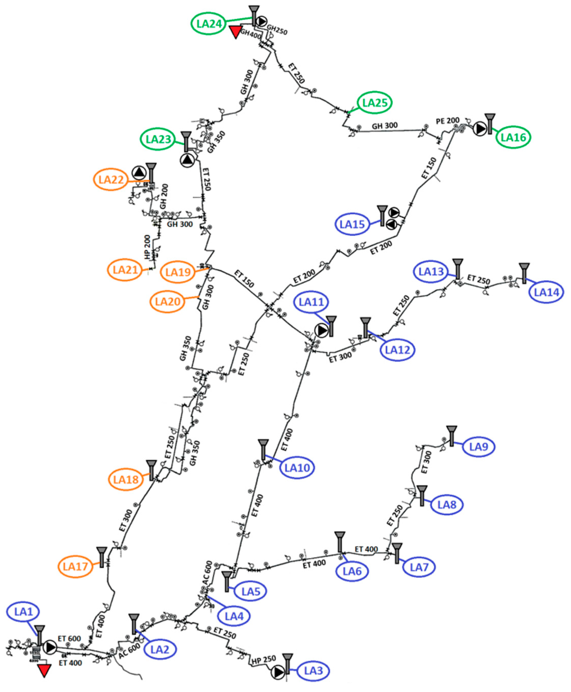
45]. The first step of modelling is the definition of the SCs in the area of interest, and in particular of the LAs, i.e., localities and districts served by the Roncocesi and Luzzara aqueducts. In this analysis, LAs, reported in
Table 3, are shown in
Figure 9, with different colors according to the SC. Three different SCs are identified in the area of interest. Here, a new “dummy” SR (SR21), with no energy and chemicals used, is added, in order to serve LA19, LA20, LA21. Water allocation coefficients, namely split coefficients, between the upstream and downstream components (e.g., WTW-SR or SC-SR), are necessary to define the topology of the system. In particular, these coefficients are used if two or more components (e.g., service reservoir) supply water to a downstream component (e.g., sub-catchment) [
46].
Table 6 lists the split coefficients between the SCs and SRs, as derived from EPANET simulations and technical reports provided by the water company. These values do not change in all the intervention strategies.
The LAs in WM2 are described by the number of inhabitants and properties, which are derived from data provided by the Water Company IREN, and ISTAT [
38,
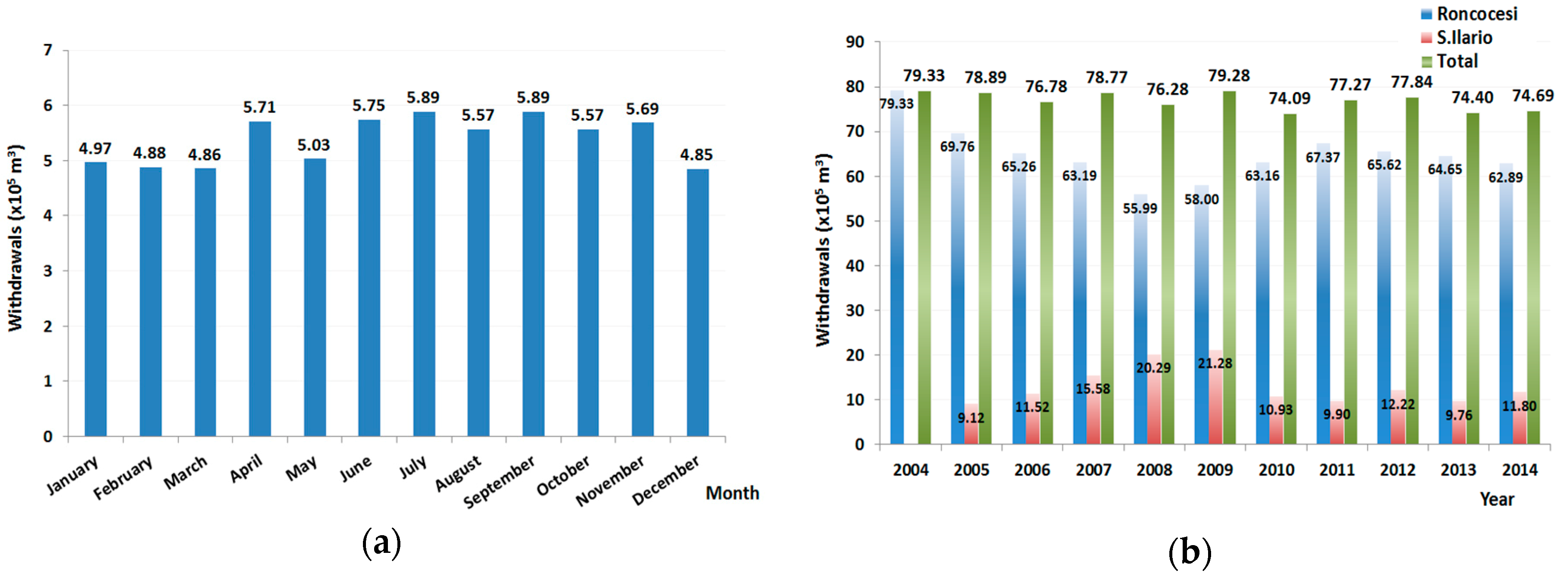
45]. The per capita indoor water demand is assessed for each LA, and the variation of the demand is assigned over the defined time horizon. The annual population increase rate assumed for the analysis represents a medium growth scenario, derived by ISTAT [
38], as depicted in
Figure 10a. Variation of the indoor water demand follows the population growth on a yearly basis, according to available predictions; in addition, monthly coefficients are applied in order to mimic seasonal variations [
47].
Per capita water consumption, leakage and other water demands, e.g., industrial and commercial, are assumed constant within the selected time horizon for all simulations. In particular, flows derived by EPANET simulations for the BAU are converted in order to obtain the total annual inflow to the WSNs for 2014, i.e., 9,210,080 m
3, with 7,456,030 m
3 belonging to the Roncocesi network, and 1,754,050 m
3 from Luzzara. The adoption of these flow values is justified by the calibration of electricity consumptions in the networks, recorded by the Italian National Electrical Energy Agency (ENEL), and available only for 2014. In particular, annual values of 718,163 kWh and 3,210,716 kWh are recorded for the Luzzara and Roncocesi water treatment plants, respectively. Data was not available for all LAs included in this study, as such where data was missing, a water demand of 190 dm
3/inhabitant/day was assumed [
45]; the adoption of this value, derived via trial and error calibration, ensures that the calculated potable water use closely matches the recorded potable water supply in the network.
Figure 10b shows the number of inhabitants served and the available/calibrated indoor water demand (dm
3/day per capita) for each LA considered in this study.
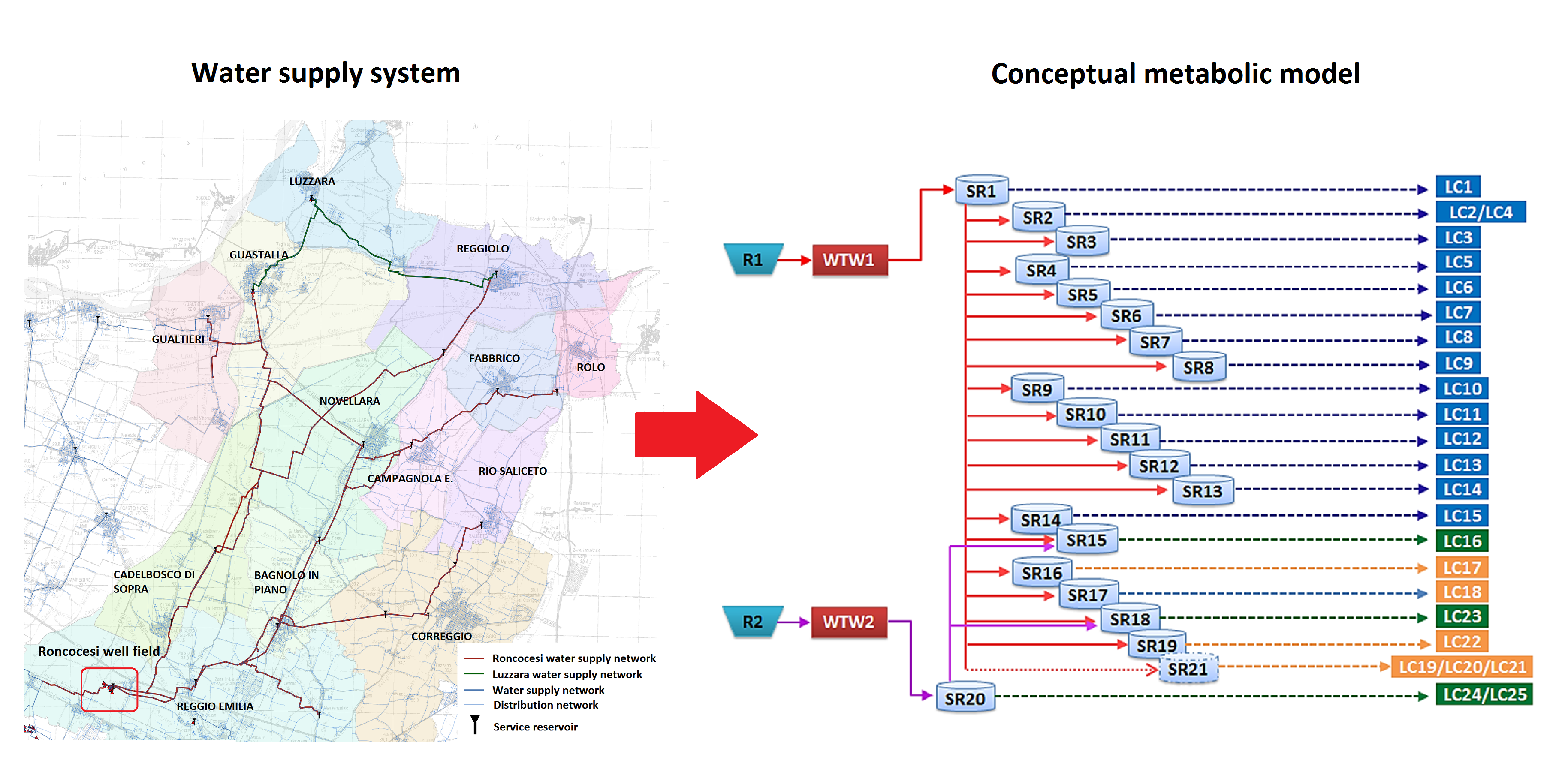
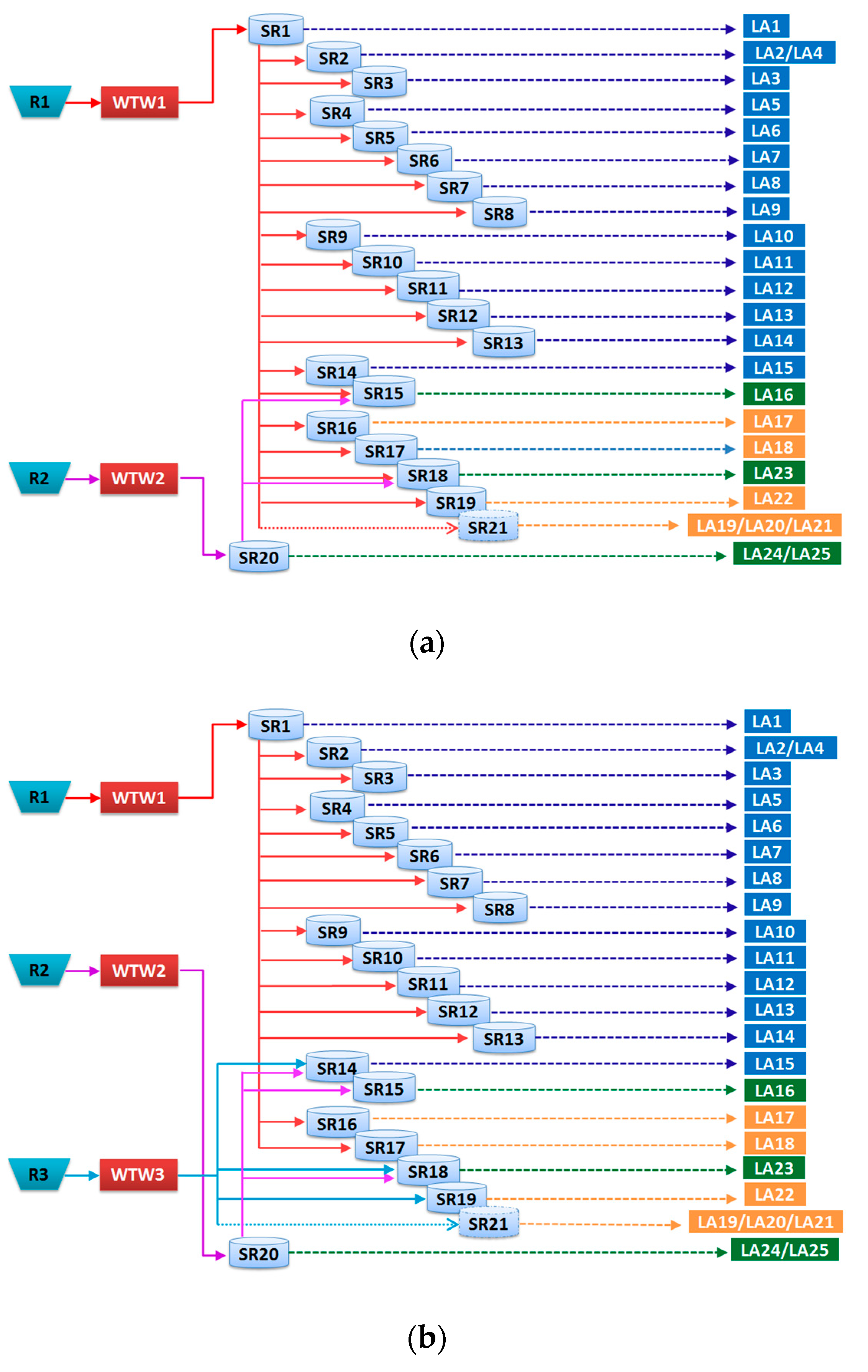
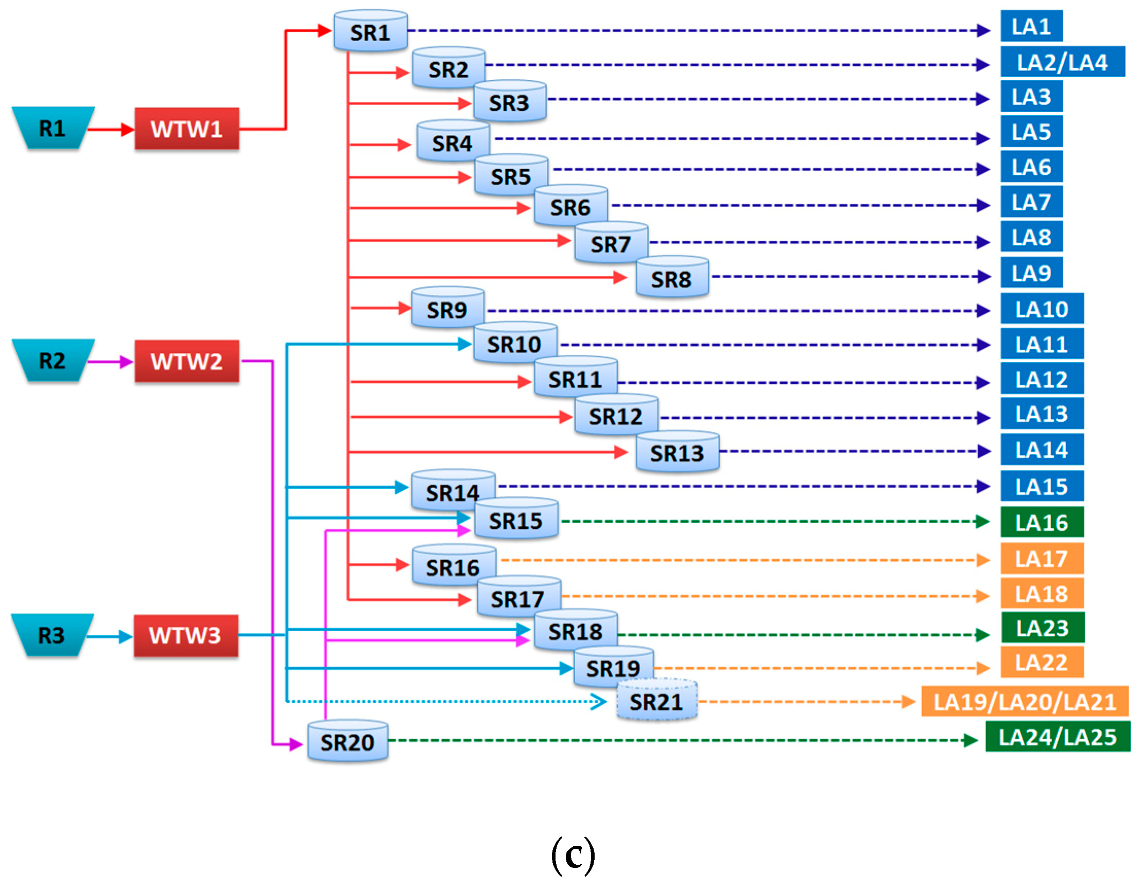
After the calibration of the indoor water demand for some LA, the topology of the water supply system is defined. The system storage components, i.e., sources, WTWs, SRs and SCs, are connected through their respective pipelines. Therefore, appropriate connections must be defined between (i) water resources and WTWs through water supply conduits, (ii) WTWs and SRs through trunk mains, and finally (iii) SRs with SCs, and their respective LAs through distribution mains. In particular, the system is fed by two main water resources in the BAU, i.e., Roncocesi (R1) and Luzzara (R2), linked to SR1 and SR20, while the other reservoirs are directly linked to the corresponding LAs. In the alternative strategies, the system configuration changes since a new water resource, i.e., Guastalla (R3) is introduced, according to the new well field. WM2 is not able to consider interconnected SRs, hence the new water resource is connected directly to the corresponding WTW and split coefficients between WTWs and the tanks are adjusted if needed.
Figure 11 depicts the conceptual models of the BAU and the alternative strategies. Here, different connections between SRs derive from the distribution of flows computed by means of EPANET simulations.
Table 7 shows the split coefficients between WTWs and SRs adopted for each simulation. These values are computed by means of EPANET simulations, based on the system performance during the time of peak demand.
After defining the schematization of the network and distribution of flows, features of the different system components are introduced. These data are related to the volume of storage components, and to the transmissivity capacity of link components. Groundwater reservoirs are considered to have infinite capacity in the model; as a result, the outflows from the well fields are assumed equal to those entering the WTWs. The transmission capacities of the water supply conduits and treatment capacity of the WTWs are computed as the sum of flows in the trunk mains leaving the WTWs, determined on the basis of an average velocity equal to 1.8 m/s. As such, it is possible to consider the trunk mains, as well as the other components of the network, as non-limiting factors for the mass balance.
Subsequently, the volumes of the SRs in the Roncocesi and Luzzara networks are estimated. Since the physical volume of the reservoirs is a limiting factor for the model, their volume is assumed equal to the transmission capacity of the relative trunk mains; if the SR is fed by more trunk mains, the sum of the transmission capacities of the trunk mains is considered. Finally, the transmission capacities of the distribution mains are computed by means of the diameters of the pipelines and assuming an average allowable velocity of 2 m/s.
It is then necessary to include an estimate of the energy and chemical consumptions within the network. Based on the values provided by the Water Company IREN, individual energy contributions in kWh/m
3 are estimated for each component of the Roncocesi and Luzzara plants. In particular, the electricity meter displays, for the year 2014, a total value of 0.43 kWh/m
3 for the Roncocesi plant, and 0.41 kWh/m
3 for the Luzzara one. These values are apportioned among the pumping wells, internal processes in the power plant (pressure filter system, backwashing, and aeration compressors), and pumping to the tanks inside the water treatment plant.
Table 8 shows the single contributions for each WTW. In particular, the energy consumption of the water treatment plant of Guastalla, associated to the new well field, is assumed to be similar to the one of Luzzara, while the average values of total head, i.e., 55 m in ST1, and 51 m in ST2, are assumed to take into account the direct pumping in the network. The energy contributions due to pumping units to the SRs are computed from EPANET simulations, which allow estimating an average operating time of individual pumps, if present, as reported in
Table 4 and
Table 5.
Table 9 lists the values of each energy contribution from pumping units, assuming an average efficiency of 65%.
Finally, the chemical concentrations of the reagents needed for the WTWs and SRs are considered. In particular, 7.5% sodium chlorite and 9% hydrochloric acid are used within the plants. In Roncocesi treatment plant, the concentrations of the two reagents is 0.004 kg/m
3, while the value for Luzzara is 0.01 kg/m
3. Since the concentration data in the SRs are not available, an average chlorine concentration of 0.01 kg/cm
3 is assumed.
Table 10 reports the default coefficients, employed in the models for the computation of energy and emissions associated with chemical compounds.

 and
and 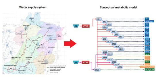


