Synergistic Approach of Remote Sensing and GIS Techniques for Flash-Flood Monitoring and Damage Assessment in Thessaly Plain Area, Greece


Abstract
:1. Introduction
2. Materials and Methods
2.1. Study Area
2.2. Background
2.3. Intensity of Rainfall from 20 to 22 May 2016
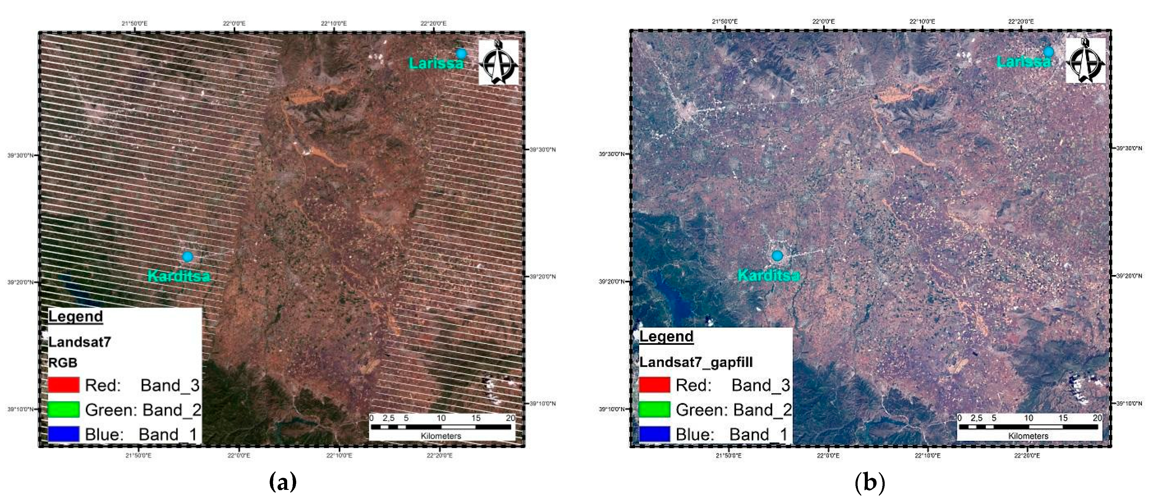
2.4. Materials
2.5. Methodology
3. Results and Discussion
4. Conclusions
Author Contributions
Funding
Acknowledgments
Conflicts of Interest
References
- Brivio, P.A.; Colombo, R.; Maggi, M.; Tomasoni, R. Integration of remote sensing data and GIS for accurate mapping of flooded areas. Int. J. Remote Sens. 2002, 23, 429–441. [Google Scholar] [CrossRef]
- Downton, M.W.; Pielke, R. Discretion without accountability: Politics, flood damage, and climate. Nat. Hazards Rev. 2001, 2, 157–166. [Google Scholar] [CrossRef]
- Jonkman, S.N.; Kelman, I. An analysis of the causes and circumstances of flood disaster deaths. Disasters 2005, 29, 75–97. [Google Scholar] [CrossRef] [PubMed]
- Golian, S.; Saghafian, B.; Maknoon, R. Derivation of Probabilistic Thresholds of Spatially Distributed Rainfall for Flood Forecasting. Water Resour. Manag. 2010, 24, 3547–3559. [Google Scholar] [CrossRef]
- Diakakis, M. A method for flood hazard mapping based on basin morphometry: Application in two catchments in Greece. Nat. Hazards 2011, 56, 803–814. [Google Scholar] [CrossRef]
- Youssef, A.M.; Pradham, B.; Hassan, A.M. Flash flood risk estimation along the St. Katherine road, southern Sinai, Egypt using GIS based morphometry and satellite imagery. Environ. Earth Sci. 2011, 62, 611–623. [Google Scholar] [CrossRef]
- Kussul, N.; Shelestov, A.; Shakun, S. Flood Monitoring from SAR Data. In Use of Satellite and In-Situ Data to Improve Sustainability; Korgan, F., Powell, A., Fedorov, O., Eds.; NATO Science for Peace and Security Series C, Environmental Security; Springer Publising Company: New York, NY, USA, 2011. [Google Scholar] [CrossRef]
- Diakakis, M.; Deligiannakis, G.; Katsetsiadou, K.; Lekkas, E.; Melaki, M.; Antoniadis, Z. Mapping and classification of direct effects of the flood of october 2014 in athens. Bull. Geol. Soc. Greece 2016, 50, 681–690. [Google Scholar] [CrossRef]
- Psomiadis, E. Flash flood area mapping utilizing Sentinel-1 radar data. In Proceedings of the SPIE Earth Resources and Environmental Remote Sensing/GIS Applications VII, Edinburgh, UK, 26–29 September 2016; p. 100051G. [Google Scholar] [CrossRef]
- Ologunorisa, T.E.; Abawua, M.J. Flood risk assessment: A review. J. Appl. Sci. Eniron. Manag. 2005, 9, 57–63. [Google Scholar]
- Munich Re. Natural Catastrophes 2015, Annual Figures. Munich Re NatCat Service, 2016. Available online: https://www.munichre.com/site/corporate/get/params_E1254966961_Dattachment/1130647/Munich-Re-Overview-Natural-catastrophes-2015.pdf (accessed on 08 February2018).
- Dong, Q.; Wang, X.; Ai, X.; Zhang, Y. Study on flood classification based on project pursuit and particle swarm optimization algorithm. J. China Hydrol 2007, 4, 10–14. [Google Scholar]
- Hooke, J.M. Variations in flood magnitude-effect relations and the implications for flood risk assessment and river management. Geomorphology 2015, 251, 91–107. [Google Scholar] [CrossRef]
- Hooke, J.M. Geomorphological impacts of an extreme flood in SE Spain. Geomorphology 2016, 263, 19–38. [Google Scholar] [CrossRef] [Green Version]
- Diakakis, M.; Mavroulis, S.; Deligiannakis, G. Floods in Greece, a statistical and spatial approach. Nat. Hazards 2012, 62, 803–814. [Google Scholar] [CrossRef]
- Psomiadis, E.; Dercas, N.; Dalezios, N.; Spyropoulos, N. The role of spatial and spectral resolution on the effectiveness of satellite-based vegetation indices. In Proceedings of the SPIE, Remote Sensing for Agriculture, Ecosystems, and Hydrology XVIII, Edinburgh, UK, 26–29 September 2016; p. 99981L. [Google Scholar]
- Frazier, P.S.; Page, J.K. Water Body Detection and Delineation with Landsat™ Data. Photogramm. Eng. Remote Sens. 2000, 66, 1461–1467. [Google Scholar]
- Klemas, V. Remote Sensing of Floods and Flood-Prone Areas: An Overview. J. Coast. Res. 2015, 31, 1005–1013. [Google Scholar] [CrossRef]
- Kussul, N.; Shelestov, A.; Shakun, S. Intelligent computations for flood monitoring. In Proceedings of the XIVth International Conference ‘Knowledge-Dialogue-Solution’ KDS, Varna, Bulgaria, 23 June–3 July 2008. [Google Scholar]
- Feyisa, G.L.; Meilby, H.; Fenshot, R.; Proud, S.R. Automated water extraction index: A new technique for surface water mapping using Landsat imagery. Remote Sens. Environ. 2014, 140, 23–35. [Google Scholar] [CrossRef]
- Clement, M.A.; Kilsby, C.G.; Moore, P. Multi-temporal synthetic aperture radar flood mapping using change detection. J. Flood Risk Manag. 2017. [Google Scholar] [CrossRef]
- Smith, L.C. Satellite remote sensing of river inundation area, stage, and discharge: A review. Hydrol. Processes 1997, 11, 1427–1439. [Google Scholar] [CrossRef]
- Li, L.; Vrieling, A.; Skidmore, A.; Wang, T.; Munoz, A.R.; Turak, E. Evaluation of MODIS Spectral Indices for Monitoring Hydrological Dynamics of a Small, Seasonally-Flooded Wetland in Southern Spain. Wetlands 2015, 35, 851–864. [Google Scholar] [CrossRef] [Green Version]
- Gao, B.C. NDWI—A normalized difference water index for remote sensing of vegetation liquid water from space. Remote Sens. Environ. 1996, 58, 257–266. [Google Scholar] [CrossRef]
- Delbart, N.; Kergoat, L.; Toan, T.L.; Lhermitte, J.; Picard, G. Determination of phenological dates in boreal regions using normalized difference water index. Remote Sens. Environ. 2005, 97, 26–38. [Google Scholar] [CrossRef]
- Xu, H.Q. Modification of normalised difference water index (NDWI) to enhance open water features in remotely sensed imagery. Int. J. Remote Sens. 2006, 27, 3025–3033. [Google Scholar] [CrossRef]
- Memon, A.; Muhammad, S.; Rahman, S.; Haq, M. Flood monitoring and damage assessment using water indices: A case study of Pakistan flood-2012. Egypt. J. Remote Sens. Space Sci. 2015, 18, 99–106. [Google Scholar] [CrossRef] [Green Version]
- Romanescu, G.; Cimpianu, C.I.; Mihu-Pintilie, A.; Stoleriu, C.C. Historic flood events in NE Romania (post-1990). J. Maps 2017, 13, 787–798. [Google Scholar] [CrossRef] [Green Version]
- Crist, E.P. A™ tasselled cap equivalent transformation for reflectance factor data. Remote Sens. Environ. 1985, 17, 301–306. [Google Scholar] [CrossRef]
- Crist, E.P.; Cicone, R.C. A Physically-Based Transformation of Thematic Mapper Data—The TMTasseled Cap. IEEE Trans. Geosci. Remote Sens. 1984, GE-22, 256–263. [Google Scholar] [CrossRef]
- Huang, C.; Wylie, B.; Yang, L.; Homer, C.; Zylstra, G. Derivation of a tasselled cap transformation based on Landsat 7 at-satellite reflectance. Int. J. Remote Sens. 2002, 23, 1741–1748. [Google Scholar] [CrossRef]
- Bhagat, V.S.; Sonawane, K.R. Use of Landsat ETM+ data for delineation of water bodies in hilly zones. J. Hydroinform. 2011, 13, 661. [Google Scholar] [CrossRef]
- Ouma, Y.O.; Tateishi, R. A water index for rapid mapping of shoreline changes of five East African Rift Valley lakes: An empirical analysis using Landsat TM and ETM + data. Int. J. Remote Sens. 2006, 27, 3153–3181. [Google Scholar] [CrossRef]
- Fisher, A.; Flood, N.; Danaher, T. Comparing Landsat water index methods for automated water classification in eastern Australia. Remote Sens. Environ. 2016, 175, 167–182. [Google Scholar] [CrossRef]
- McFeeters, S.K. The use of the Normalized Difference Water Index (NDWI) in the delineation of open water features. Int. J. Remote Sens. 1996, 17, 1425–1432. [Google Scholar] [CrossRef]
- Xiao, X.; Boles, S.; Frolking, S.; Salas, W.; Moore, B., III; Li, C.; He, L.; Zhao, R. Observation of flooding and rice transplanting of paddy rice fields at the site to landscape scales in China, using VEGETATION sensor data. Int. J. Remote Sens. 2002, 23, 3009–3022. [Google Scholar] [CrossRef]
- Devranche, A.; Poulin, B.; Lefebvre, G. Mapping flooding regimes in Camargue wetlands using seasonal multispectral data. Remote Sens. Environ. 2013, 138, 165–171. [Google Scholar] [CrossRef] [Green Version]
- Rogers, A.S.; Kearney, M.S. Reducing signature variability in unmixing coastal marsh thematic mapper scenes using spectral indices. Int. J. Remote Sens. 2004, 25, 2317–2335. [Google Scholar] [CrossRef]
- Gond, V.; Bartholomé, E.; Ouattara, F.; Nonguierma, A.; Bado, L. Surveillance et cartographie des plans d’eau et des zones humides et inondables en régions arides avec l’instrument VEGETATION embarqué sur SPOT-4. Int. J. Remote Sens. 2004, 25, 987–1004. [Google Scholar] [CrossRef]
- Earth.esa.int, 2015. User Guides—Sentinel-2 MSI—Overview—Sentinel Online. 2017. Available online: https://earth.esa.int/web/sentinel/user-guides/sentinel-2-msi/overview (accessed on 8 February 2018).
- Chatziantoniou, A.; Petropoulos, G.P.; Psomiadis, E. Co-Orbital Sentinel 1 and Sentinel 2 for LULC Mapping with Emphasis in a Mediterranean Setting Based on Machine Learning. Remote Sens. 2017, 9, 1259. [Google Scholar] [CrossRef]
- Matgen, P.; Schumann, G.; Henry, J.B.; Hoffmann, L.; Pfister, L. Integration of SAR-derived river inundation areas, high-precision topographic data and a river flow model toward near real-time flood management. Int. J. Appl. Earth Obs. Geoinf. 2007, 9, 247–263. [Google Scholar] [CrossRef]
- Kiage, L.M.; Walker, N.D.; Balasubramanian, S.; Baras, J. Application of Radarsat-1 synthetic aperture radar imagery to assess hurricane-related flooding of coastal Louisiana. Int. J. Remote Sens. 2005, 26, 5359–5380. [Google Scholar] [CrossRef]
- Hess, L.L.; Melack, J.M.; Filoso, S.; Wang, Y. Delineation of inundated area and vegetation along the Amazon floodplain with the SIR-C synthetic aperture radar. IEEE Trans. Geosci. Remote Sens. 1995, 33, 896–904. [Google Scholar] [CrossRef]
- Giustarini, L.; Hostache, R.; Matgen, P.; Schumann, G.J.P.; Bates, P.D.; Mason, D.C. A change detection approach to flood mapping in urban areas using TerraSAR-X. IEEE Trans. Geosci. Remote Sens. 2013, 51, 2417–2430. [Google Scholar] [CrossRef]
- MacIntosh, H.; Profeti, G. The use of ERS SAR data to manage flood emergencies at the smaller scale. In Proceedings of the 2nd ERS Applications Workshop, European Space Agency, London, UK, 6–8 December 1995; pp. 243–246. [Google Scholar]
- Schumann, G.; Henry, J.B.; Hoffmann, L.; Pfister, L.; Pappenberger, F.; Matgen, P. Demonstrating the high potential of remote sensing in hydraulic modelling and flood risk management. In Proceedings of the Annual Conference of the Remote Sensing and Photogrammetry Society with the NERC Earth Observation Conference, Portsmouth, UK, 6–9 September 2005. [Google Scholar]
- Stevens, T.B. Synthetic Aperture Radar for Coastal Flood Mapping. NASA Global Change Master Directory; Data Originator; LSU Earth Scan Laboratory: Baton Rouge, LA, USA, 2013; Available online: http://www.esl.lsu.edu/ (accessed on 14 February 2018).
- Henry, J.-B.; Chastanet, P.; Fellah, K.; Densos, Y.-L. Envisat multipolarized ASAR for flood mapping. Internation. J. Remote Sens. 2006, 27, 1921–1929. [Google Scholar] [CrossRef]
- Schumann, G.; Bates, P.D.; Horritt, M.S.; Matgen, P.; Pappenberger, F. Progress in integration of remote sensing-derived flood extent and stage data and hydraulic models. Rev. Geophys. 2009, 47, RG4001. [Google Scholar] [CrossRef]
- Schlaffer, S.; Matgen, P.; Hollaus, M.; Wagner, W. Flood detection from multi-temporal SAR data using harmonic analysis and change detection. Int. J. Appl. Earth Obs. Geoinf. 2015, 38, 15–24. [Google Scholar] [CrossRef]
- Ferrant, S.; Selles, A.; Page, L.M.; Herrault, P.-A.; Pelletier, C.; Al-Bitar, A.; Mermoz, S.; Gascoin, S.; Bouvet, A.; Saqalli, M.; et al. Detection of Irrigated Crops from Sentinel-1 and Sentinel-2 Data to Estimate Seasonal Groundwater Use in South India. Remote Sens. 2017, 9, 1119. [Google Scholar] [CrossRef]
- Jain, S.K.; Singh, R.D.; Jain, M.K.; Lohani, A.K. Delineation of flood-prone areas using remote sensing techniques. Water Resour. Manag. 2005, 19, 333–347. [Google Scholar] [CrossRef]
- Liu, W.; Yamazaki, F. Review article: Detection of inundation areas due to the 2015 kanto and tohoku torrential rain in japan based on multi-temporal ALOS-2 imagery. Nat. Hazards Earth Syst. Sci. 2018, 18, 1905–1918. [Google Scholar] [CrossRef]
- Lyu, H.; Wang, G.; Shen, J.S.; Lu, L.; Wang, G. Analysis and GIS mapping of flooding hazards on 10 may 2016, guangzhou, china. Water 2016, 8, 447. [Google Scholar] [CrossRef]
- Chen, B.; Krajewski, W.F.; Goska, R.; Young, N. Using LiDAR surveys to document floods: A case study of the 2008 Iowa flood. J. Hydrol. 2017, 553, 338–349. [Google Scholar] [CrossRef]
- Qian, T.; Shen, D.; Xi, C.; Chen, J.; Wang, J. Extracting farmland features from LiDAR-derived DEM for improving flood plain delineation. Water 2018, 10, 252. [Google Scholar] [CrossRef]
- Vesakoski, J.; Alho, P.; Hyyppä, J.; Holopainen, M.; Flener, C.; Hyyppä, H. Nationwide digital terrain models for topographic depression modelling in detection of flood detention areas. Water 2014, 6, 271–300. [Google Scholar] [CrossRef]
- Zoka, M.; Psomiadis, E.; Dercas, N. The complementary use of Optical and SAR data in monitoring flood events and their effects. Proceedings 2018, 2, 644. [Google Scholar] [CrossRef]
- Tsouni, A.; Kontoes, C.; Koutsoyiannis, D.; Mamassis, N.; Elias, P. Estimation of Actual Evapotranspiration by Remote Sensing: Application in Thessaly Plain, Greece. Sensing 2008, 8, 3586–3600. [Google Scholar] [CrossRef] [PubMed] [Green Version]
- Demitrack, A. The Late Quaternary Geologic History of the Larissa Plain Thessaly, Greece: Tectonic, Climatic, and Human Impact on the Landscape Soil Stratigraphy, Neolithic Period, Pinios River, Uranium/Thorium Disequilibrium Dating. Ph.D. Thesis, Stanford University, Stanford, CA, USA, 1986. [Google Scholar]
- Orengo, H.A.; Krahtopoulou, A.; Garcia-Molsosa, A.; Palaiochoritis, K.; Stamati, A. Photogrammetric re-discovery of the hidden long-term landscapes of western Thessaly, central Greece. J. Archaeol. Sci. 2015, 64, 100–109. [Google Scholar] [CrossRef]
- Ministry of Environment and Energy of Greece. Available online: http://www.ypeka.gr/Default.aspx?tabid=37&locale=en-US (accessed on 9 February 2018).
- National Observatory of Athens. Available online: http://meteosearch.meteo.gr/stationInfo.asp (accessed on 14 February 2018).
- Earth Explorer. Available online: https://earthexplorer.usgs.gov/ (accessed on 8 February 2018).
- Copernicus Open Access Hub. Available online: https://scihub.copernicus.eu/ (accessed on 21 February 2018).
- Hellenic Military Geographical Service (HMGS). Topographic Maps, Scale 1:5.000; HMGS: Athens, Greece, 1988. [Google Scholar]
- OPEKEPE Integrated Administration and Control System, Payment and Control Agency for Guidance and Guarantee Community Aid, Ministry of Agricultural Development and Food, Athens, Greece. Available online: http://www.opekepe.gr/ (accessed on 2 March 2018).
- Roupioz, L.; Nerry, F.; Jia, L.; Menenti, M. Improved surface reflectance from remote sensing data with sub-pixel topographic information. Remote Sens. 2014, 6, 10356–10374. [Google Scholar] [CrossRef]
- Théau, J.; Sankey, T.; Weber, T.K. Multi-sensor Analyses of vegetation indices in a semi-arid environment. GISci. Remote Sens. 2010, 47, 260–275. [Google Scholar] [CrossRef]
- Harris Geospatial Solutions. Available online: http://www.harrisgeospatial.com/docs/QUAC.html (accessed on 21 February 2018).
- ESA Sentinel Online. User Guides—Sentinel-2 MSI—Overview, 2017. Available online: https://earth.esa.int/web/sentinel/user-guides/sentinel-2-msi/overview (accessed on 31 January 2018).
- Kauth, R.J.; Thomas, G.S. The tasselled cap—A graphic description of the spectral temporal development of agricultural crops as seen by LANDSAT. In Proceedings of the Symposium Machine Processing of Remote Sensing Data, West Lafayette, IN, USA, 29 June–1 July 1976. [Google Scholar]
- Rouse, J.W.; Haas, R.H.; Schell, J.A.; Deering, D.W. Monitoring the Vernal Advancement and Retrogradation (Green Wave Effect) of Natural Vegetation; NASA/GSFC Type III Final Report; NASA: Greenbelt, MD, USA, 1974; p. 371.
- Viches, J.P. Detection of Areas Affected by Flooding River using SAR images. In Seminar: Master in Space Applications for Emergency Early Warning and Response; Consiglio Nazionale delle Ricerche (CNR) -Istituto di Metodologieper l’Analisi Ambientale (IMAA): Rome, Italy, 2013; p. 40. [Google Scholar]
- Lee, J.S.; Pottier, E. Polarimetric SAR Radar Imaging: From Basic to Applications; CRC Press, Taylor & Francis Group: Boca Raton, FL, USA, 2009. [Google Scholar]
- Graf, L.Q.; Moreno-de-las-Heras, M.; Ruiz, M.; Calsamiglia, A.; García-Comendador, J.; Fortesa, J.; Estrany, J. Accuracy assessment of digital terrain model dataset sources for hydrogeomorphological modelling in small mediterranean catchments. Remote Sens. 2018, 10, 2014. [Google Scholar] [CrossRef]
- Jenson, S.K.; Domingue, J.O. Extracting topographic structure from digital elevation data for geographic information-system analysis. Photogramm. Eng. Remote Sens. 1988, 54, 1593–1600. [Google Scholar]
- Soulis, K.X. . Development of a simplified grid cells ordering method facilitating GIS-based spatially distributed hydrological modeling. Comput. Geosci. 2013, 54, 160–163. [Google Scholar] [CrossRef]
- Soulis, K.X.; Kalivas, D.P.; Apostolopoulos, C. Delimitation of agricultural areas with natural constraints in Greece: Assessment of the dryness climatic criterion using geostatistics. Agronomy 2018, 8, 161. [Google Scholar] [CrossRef]
- Greek Agricultural Insurance Organization. Available online: http://www.elga.gr/ (accessed on 21 February 2018).
- Jeyaseelan, A.T. Drought & flood assessment and monitoring using remote sensing and GIS. In Satellite remote Sensing and GIS Applications in Agricultural Meteorology; Dun, D., Ed.; World Meteorological Organization: Hyderabad, India; Geneva, Switzerland, 2003; p. 291. [Google Scholar]
- Haq, M.; Akhtar, M.; Muhammad, S.; Paras, S.; Rahmatullah, J. Techniques of Remote Sensing and GIS for flood monitoring and damage assessment: A case study of Sindh province, Pakistan. Egypt. J. Remote Sens. Space Sci. 2012, 15, 135–141. [Google Scholar] [CrossRef] [Green Version]
- Schunmann, G.; Moller, D.K. Microwave remote sensing of flood inundation. Phys. Chem. Earth 2015, 83–84, 85–95. [Google Scholar] [CrossRef]


| Satellite System | Instrument | Image Code/Source | Acquisition Date | Use | |
|---|---|---|---|---|---|
| Landsat 7 | ETM+ | LE71840332016144NSG00 | 23 May 2016 | Flood monitoring | |
| Sentinel-1 | C-SAR | S1A_IW_GRDH_1SDV_20160521T043901_20160521T043926_011352_0113BF_4FE4 | 21 May 2016 T07:03:18 | Flood monitoring | |
| Sentinel-2 | MSI | S2A_OPER_PRD_MSIL1C_PDMC_20151206T141435_R093_V20151206T093115_20151206T093115 | 6 December 2015 | Land Cover Classification | |
| S2A_OPER_PRD_MSIL1C_PDMC_20160406T143016_R093_V20160404T092409_20160404T092409 | 4 April 2016 | ||||
| S2A_USER_MTD_SAFL2A_PDMC_20160713T145354_R093_V20160713T092032_20160713T092032 | 13 July 2016 | ||||
| S2A_USER_MTD_SAFL2A_PDMC_20160812T184246_R093_V20160812T092032_20160812T092031 | 12 August 2016 | ||||
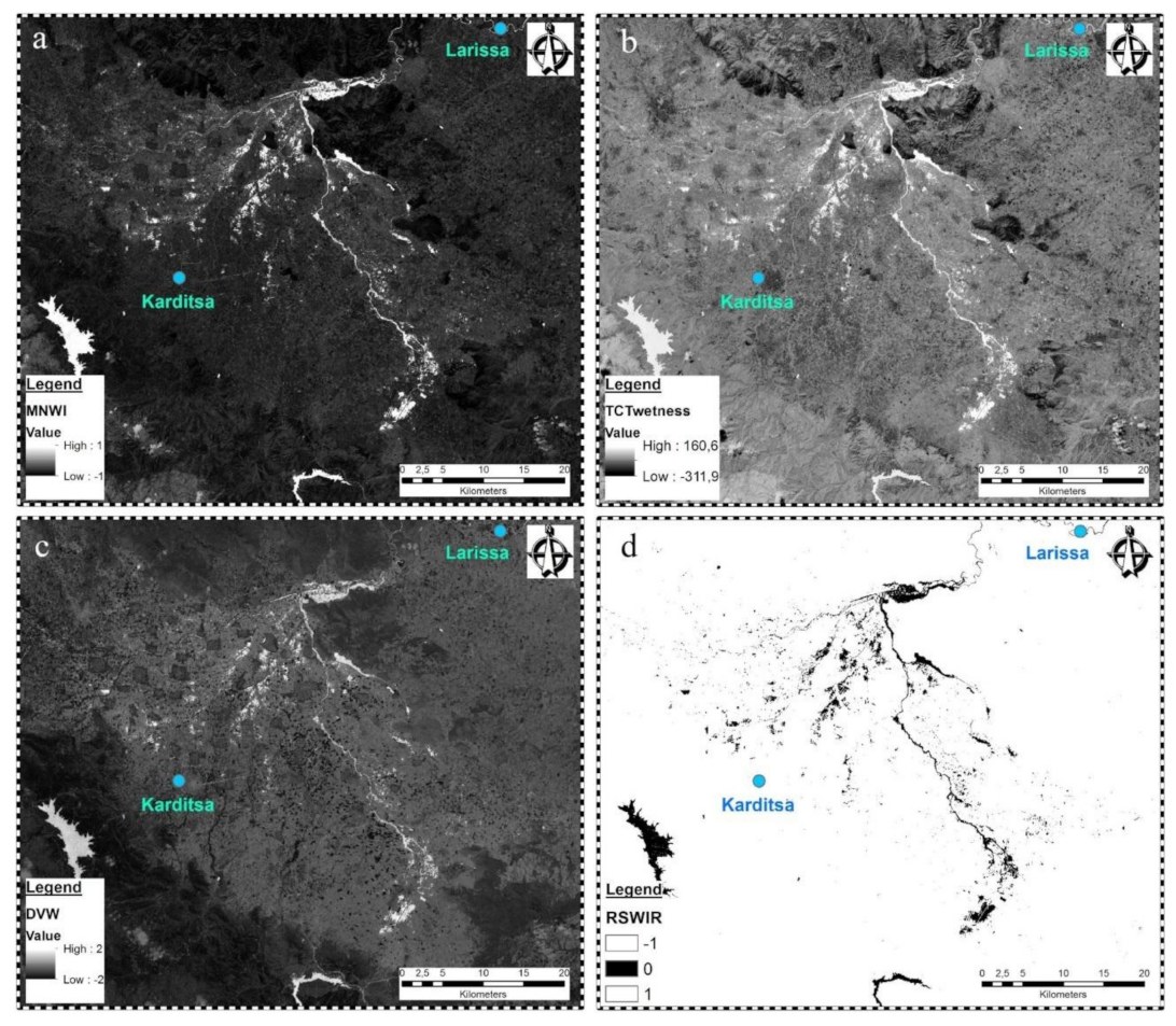
| Indices | Equation | References |
|---|---|---|
| NDWI—Normalized Difference Water Index | (GREEN − NIR)/(GREEN + NIR) | Gao 1996 [24] |
| MNDWI—Modified Normalized Difference Water Index | (GREEN − MIR)/(GREEN + MIR) | Xu 2006 [26] |
| NDVI—Normalized Difference Vegetation Index | (NIR − RED)/(NIR + RED) | Rouse et al. 1974 [74] |
| DVW—Vegetation and Water Index | NDVI − NDWI | Gond et al. 2004 [39] |
| RSWIR—Red and Short Wave Infrared Index | (RED − SWIR)/(RED + SWIR) | Rogers & Kearney 2004 [38] |
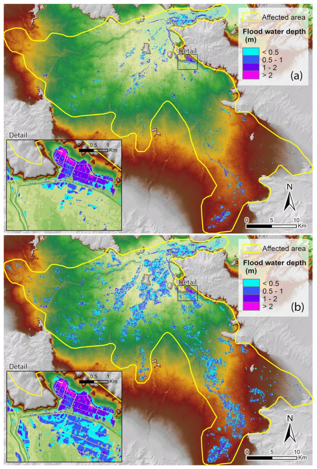
| Original | Clipped to Parcels | |||
|---|---|---|---|---|
| Depth | RS | Extended | RS | Extended |
| (m) | (m2) | (m2) | (m2) | (m2) |
| <0.5 | 17,637,200 | 81,388,900 | 15,052,100 | 68,525,900 |
| 0.5–1.0 | 19,159,300 | 75,632,000 | 16,665,100 | 64,701,000 |
| 1.0–2.0 | 10,526,900 | 30,376,500 | 8,034,700 | 23,390,500 |
| >2.0 | 1,212,700 | 1,896,300 | 211,500 | 306,300 |
| Sum | 48,536,100 | 189,293,700 | 39,963,400 | 156,923,700 |
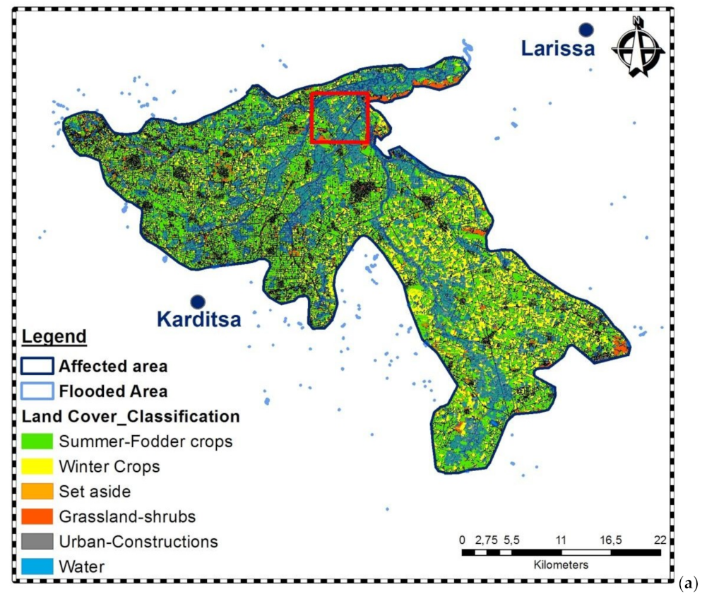
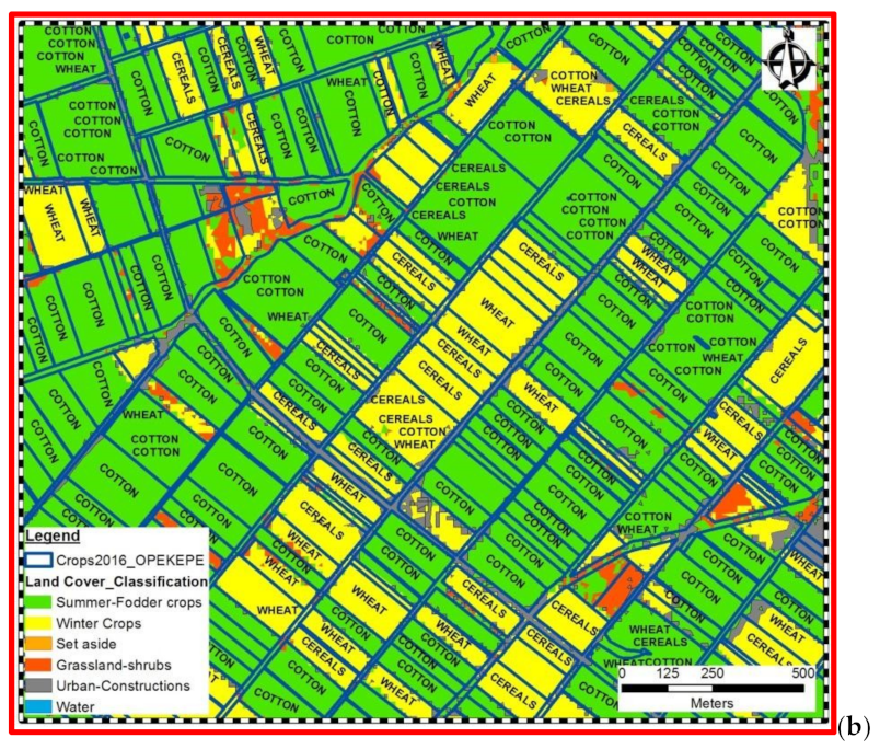
| Crop | Affected areas | |||||
|---|---|---|---|---|---|---|
| ELGA | RS | Extended | ||||
| (m2) | (%) | (m2) | (%) | (m2) | (%) | |
| Cotton | 30,208,336 | 79 | 27,954,900 | 73 | 92,537,700 | 61 |
| Winter Cereals | 4,588,608 | 12 | 4,456,900 | 12 | 34,590,300 | 23 |
| Corn | 1,529,536 | 4 | 2,563,100 | 7 | 6,916,200 | 5 |
| Fodder | 382,384 | 1 | 2,348,100 | 6 | 12,338,900 | 8 |
| Other crops | 1,529,536 | 4 | 1,067,300 | 3 | 5,489,600 | 4 |
| SUM | 38,238,400 | 100 | 38,390,300 | 100 | 151,872,700 | 100 |
© 2019 by the authors. Licensee MDPI, Basel, Switzerland. This article is an open access article distributed under the terms and conditions of the Creative Commons Attribution (CC BY) license (http://creativecommons.org/licenses/by/4.0/).
Share and Cite
Psomiadis, E.; Soulis, K.X.; Zoka, M.; Dercas, N. Synergistic Approach of Remote Sensing and GIS Techniques for Flash-Flood Monitoring and Damage Assessment in Thessaly Plain Area, Greece. Water 2019, 11, 448. https://doi.org/10.3390/w11030448
Psomiadis E, Soulis KX, Zoka M, Dercas N. Synergistic Approach of Remote Sensing and GIS Techniques for Flash-Flood Monitoring and Damage Assessment in Thessaly Plain Area, Greece. Water. 2019; 11(3):448. https://doi.org/10.3390/w11030448
Chicago/Turabian StylePsomiadis, Emmanouil, Konstantinos X. Soulis, Melpomeni Zoka, and Nicholas Dercas. 2019. "Synergistic Approach of Remote Sensing and GIS Techniques for Flash-Flood Monitoring and Damage Assessment in Thessaly Plain Area, Greece" Water 11, no. 3: 448. https://doi.org/10.3390/w11030448