Investigating Spatial and Temporal Variation of Hydrological Processes in Western China Driven by CMADS


1
College of Resources and Environmental Sciences, Xinjiang University (XJU), Urumqi 830046, China
2
Department of Geography, Shihezi University, Shihezi 832000, Xinjiang, China
3
China Institute of Water Resource and Hydropower Research (IWHR), Beijing 100038, China
*
Authors to whom correspondence should be addressed.
Water 2019, 11(3), 435; https://doi.org/10.3390/w11030435
Submission received: 28 December 2018
/
Revised: 13 February 2019
/
Accepted: 18 February 2019
/
Published: 28 February 2019
(This article belongs to the Special Issue Application of the China Meteorological Assimilation Driving Datasets for the SWAT Model (CMADS) in East Asia)
Abstract
:The performance of hydrological models in western China has been restricted due to the scarcity of meteorological observation stations in the region. In addition to improving the quality of atmospheric input data, the use hydrological models to analyze Hydrological Processes on a large scale in western China could prove to be of key importance. The Jing and Bortala River Basin (JBR) was selected as the study area in this research. The China Meteorological Assimilation Driving Datasets for the SWAT model (CMADS) is used to drive SWAT model, in order to greatly improve the accuracy of SWAT model input data. The SUFI-2 algorithm is also used to optimize 26 sensitive parameters within the SWAT-CUP. After the verification of two runoff observation and control stations (located at Jing and Hot Spring) in the study area, the temporal and spatial distribution of soil moisture, snowmelt, evaporation and precipitation were analyzed in detail. The results show that the CMADS can greatly improve the performance of SWAT model in western China, and minimize the uncertainty of the model. The NSE efficiency coefficients of calibration and validation are controlled between 0.659–0.942 on a monthly scale and between 0.526–0.815 on a daily scale. Soil moisture will reach its first peak level in March and April of each year in the JBR due to the snow melting process in spring in the basin. With the end of the snowmelt process, precipitation and air temperature increased sharply in the later period, which causes the soil moisture content to fluctuate up and down. In October, there was a large amount of precipitation in the basin due to the transit of cold air (mainly snowfall), causing soil moisture to remain constant and increase again until snowmelt in early spring the following year. This study effectively verifies the applicability of CMADS in western China and provides important scientific and technological support for the spatio-temporal variation of soil moisture and its driving factor analysis in western China.
1. Introduction
In recent years, there have been a number of serious ecological and water crises in the world, with changes to the land surface process in arid areas having a significant influence on the whole inland river water cycle and the ecological environment of vast areas. These changes include arid inland water, the water quality and the continuous degradation, all of which make a frequent contribution to adverse water events. Due to the unique structure of arid oases, their water and energy cycles have their own laws, and local climate conditions are inextricably linked to them. Therefore, it is necessary to systematically analyze the temporal and spatial variations of the surface hydrological components in the arid areas of Xinjiang, which may provide important technical support for the ecological and hydrological restoration and sustainable development of arid areas.
The JBR are located in Xinjiang, western China, and their basins enclose the total area of the surface’s hydrological components’ spatial variation in the arid alpine area of Xinjiang; the middle of this area is a valley, whilst the east is a basin. Furthermore, its geomorphology and terrain can be connected with the Junggar Basin and divided into three major types of landforms: mountain, valley, and basin. Because the watershed interchanges are located in the sinking area of the Alashan Mountain, wind is the largest meteorological hazard in the Bo River Basin. Due to the fragile ecological structure of the basin, the impact of both salinization and desertification is serious. In recent years, with climate change and large-scale human reclamation activities, the amount of water flowing into the Ebinur Lake in the JBR has decreased and the ecological environment has continued to degenerate. According to statistics, between the 1950s and 1970s, the Ebinur Lake in the JBR shrunk in size by nearly 678 square kilometers, and lost nearly 2.3 billion cubic meters of water. Due to the sharp decline in water resources, the lake’s salinity has greatly increased, the wetland area has become smaller, and the lake’s role in climate regulation has reduced, which is devastating to both the ecosystem and local residents. The impact of this makes the already very fragile ecological environment of the JBR further deteriorate, resulting in a biological chain chasm, reduced biological diversity, intensified desertification and other ecological problems. As the JBR contributes greatly to the ecological balance and social economy in Xinjiang, it is vital to develop the surface related parameters (such as the ecological hydrological parameters) of the JBR and provide the locality with feasible and sustainable development based on the simulation of the land surface process. However, due to the scarcity of traditional observation sites in the region, large differences in the underlying surface, and the increased influence of climate change and human activities, it is difficult to simulate the temporal and spatial changes of the surface components in Xinjiang. In other words, the uncertainty of the atmospheric-related data will lead to a significant increase in the uncertainty of the region’s analog output [1].
Numerous analyses have shown that if the atmospheric dataset contains more observation data, the simulation results can be improved significantly [2,3,4,5,6,7,8,9,10,11,12,13,14,15,16]. The NCEP and NCAR are cooperating in a project denoted “reanalysis” to produce a 40-year record of global analyses of atmospheric fields in support of the needs of the research and climate monitoring communities. ERA is a re-analysis of meteorological observations from September 1957 to August 2002 produced by the European Centre for Medium-Range Weather Forecasts (ECMWF) in collaboration with many institutions. There are currently many kinds of atmospheric datasets in use in China and overseas, such as the NCAR/DOE of NCEP [17,18], ERA-15, ERA-40, ERA-Interim reanalysis data [19], JRA-25 reanalysis data [20] and the Princeton dataset, all of which can enhance the model’s performance. As traditional atmospheric observing stations do not cover the whole world, the above datasets provide an important basis for data analysis [17]. However, despite the continuous emergence of various types of atmospheric reanalysis datasets or atmospheric-driven fields, these datasets need to be further validated for a study of large and medium-sized areas. For example, Jeremy et al. used the regional climate model (RegCM) to simulate and evaluate the monthly variation of precipitation in the winter and summer seasons in the East Asian monsoon region, and found that the RegCM model made large errors when forecasting precipitation. It is believed that this phenomenon is particularly evident in winter. Furthermore, numerous studies have shown that NCEP, ERA and JRA reanalysis datasets can leads to obvious seasonal and regional differences over China [21,22,23,24,25,26,27,28]. For example, Shi et al. [29] used various technical means to evaluate the usability of NCAR-driven data (e.g., air temperature, wind speed) in China, with their results showing that the wind field anomalies were negatively correlated with altitude. Ning et al. [30] used Noah LSM-HMS driven by model (CMADS) with a very good performance, indicating that streamflow is increased in dry seasons and decreased in wet seasons, and large and small reservoirs can have equally large effects on the streamflow.
The above studies have proved that although all kinds of reanalysis products and datasets can reflect large-scale meteorological elements; however, for China, especially the western region, the regional surface differences are large and observation stations are relatively scarce. Moreover, most of the reanalysis datasets used in previous research have not been assimilated with data from the regional automatic stations within China; therefore, they are unable to reflect the strength and frequency of the various driving factors effectively [31]. In summary, it is very important to simulate and analyze the relevant surface components by using a meteorological background field which has been corrected by a regional automatic station so as to develop a more credible hydrological simulations [32,33].
The China Meteorological Assimilation Datasets for the SWAT model (CMADS) was completed over the 9-year period of 1 January 2008 through 31 December 2016, and has been used in many watersheds throughout East Asia [34,35,36,37,38,39,40,41,42,43]. Furthermore, Researchers from China also used CMADS data and Penman-Monteith method to calculate Potential evapotran-spiration (PET) across China with good performance [44,45,46,47,48,49,50,51]. However, although CMADS has many applications in China, there are few applications in western China, where traditional weather stations are scarce. Especially in the western part of China, the surface space-time differentiation and complexity, coupled with the region’s economic and other objective factors, limit the local establishment of a large number of meteorological observation systems [50,51,52]. Therefore, the use of limited traditional observatories by local scientists does not for the basis for good scientific and effective study of the local underlay surface. Since analyses of surface processes (such as soil moisture, temperature, melting snow, etc.) based on the CMADS+ SWAT mode are not being used very well until now, the purpose of this paper is try to use high-precision meteorological data (CMADS) to drive the SWAT model. When the SWAT model is localized, we will effectively analyze and examine other surface processes (snowmelt, soil moisture, etc.).
2. Study Area
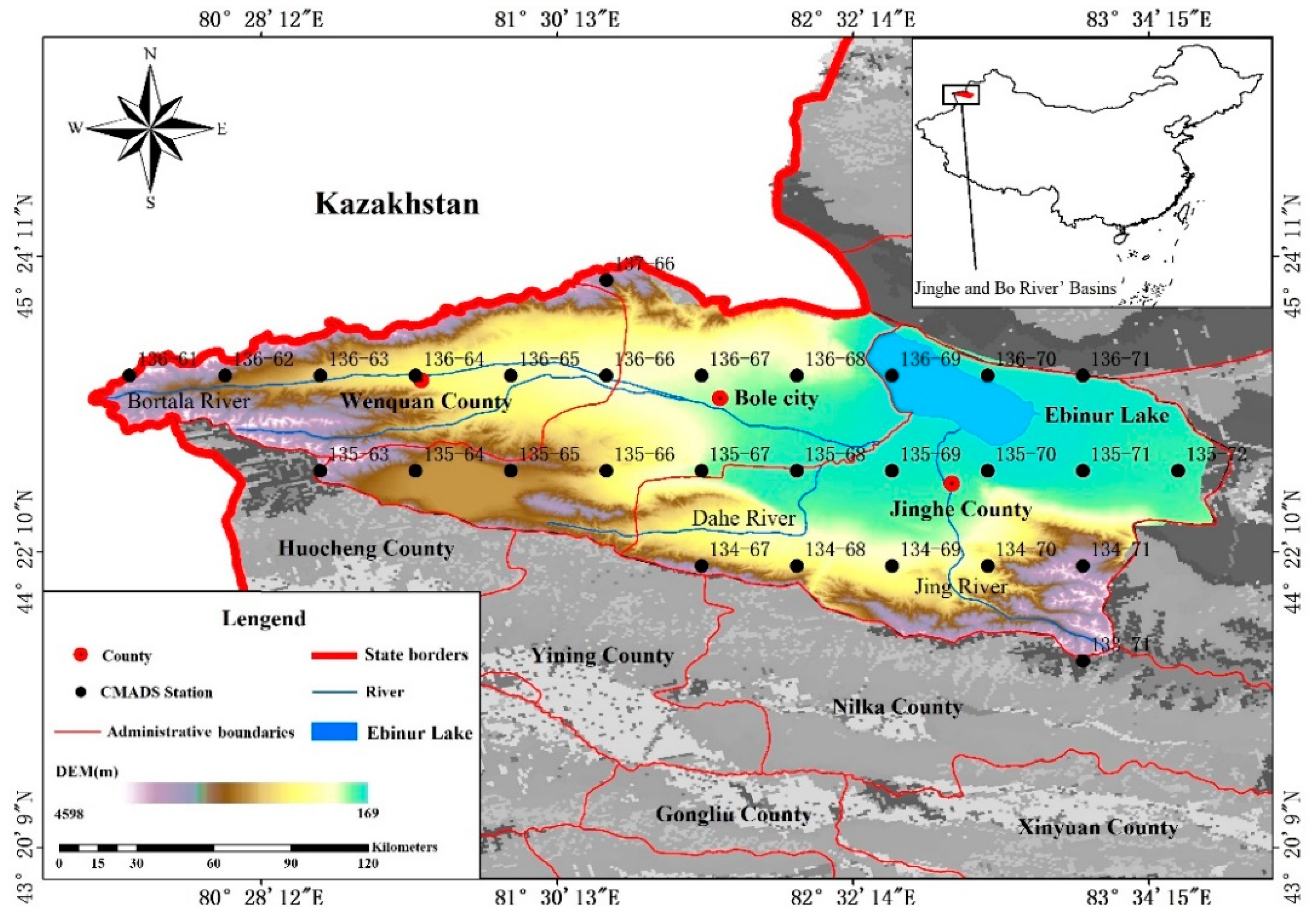
The JBR are located on the northern slope of the western Tianshan Mountains (Figure 1), (81°46’–83°51’ E, 44°02’–45°10’ N), with a total area of 11,300 km2. The precipitation is mostly from the Arctic Ocean and the Atlantic water vapor, and shows an overall pattern of (1) more in the mountains than the plains, (2) more in the west than the east, and (3) more along the shady slope than the sunny slope. The basin has a distribution of nearly 460 glaciers, with a total of 15.4 km2 of glacier reserves. Among them, the glacier areas in the JBR regions reach 96.2 km2 and 110.3 km2 respectively. The amount of glacier replenishment in the Jinghe is about 96 million m3, whilst in the Bo River it is about 105 million m3, accounting for 20.6% and 21.4% of their total river runoffs respectively. The combined effects of temperature, precipitation and topography have led to the runoff replenishment of the region depending mainly on snow, ice, rainfall and groundwater, making the area a typical arid basin. However, the mineralization of Ebinur Lake has gradually increased in recent years, and the competition between ecological and domestic water usage has become increasingly intensive. In addition, the land degradation within the basin is also very serious, and 1500 km2 of the underwater region of the Ebinur Lake has been degraded into a salt desert, with a salinization area of 71 km2.
In recent years, researchers have only used various types of reanalysis data (or regional climate models) and single point observation data to study the JBR and the whole Xinjiang region. As the Xinjiang regional meteorological stations are relatively scarce, the region has not yet undergone a more thorough and reliable simulation and analysis of the hydrological process. However, it is very important that the temporal and spatial evolution of the hydrological correlation components are simulated using the SWAT model, which has a high resolution and reliable driving field.
3. Material and Methods
3.1. Material
The China Meteorological Assimilation Driving Datasets for the SWAT model (CMADS) is a public datasets developed by Xianyong Meng from China agriculture university (http://www.cmads.org/).The input datasets for the SWAT model mainly includes land use, the river network, digital elevation model (DEM) and soil distribution, as well as other data (Figure 2). Among them, the SRTM90mdigital elevation is obtained from the CGIAR-CSI SRTM database: (http://srtm.csi.cgiar.org/SELECTION/input Coord.asp).
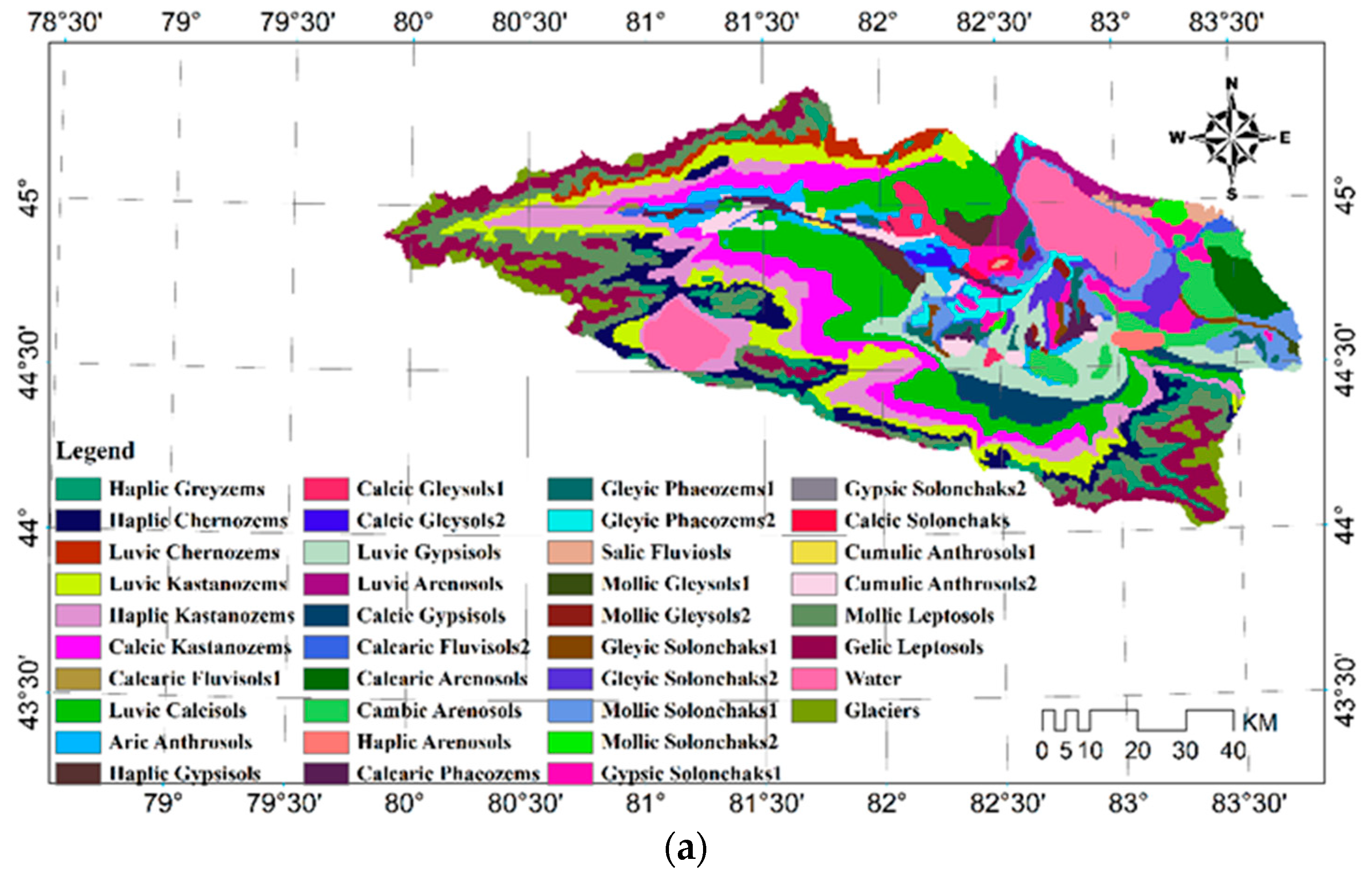
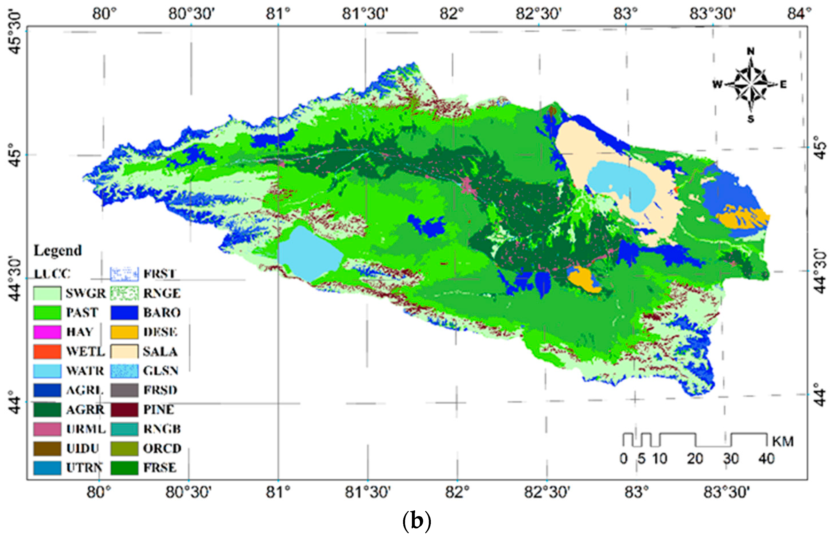
The physical properties of soil determines the characteristics of the production and confluence of the different hydrological units in the SWAT model, and also provide a reference for the definition of the hydrological response unit (HRU). The soil input data selected in this study is the Harmonized World Soil Database version 1.1 (HWSD 1.1), which has been derived from the World Soil Database (HWSD). The land use comes from the Management Office of the JBR. The distribution of the original land use data in the study area is analyzed in the JBR (see Figure 3B). The land use data is superimposed on the Second Glacier Inventory Dataset of China (Version 1.0) [25].
In order to ensure the consistency of the resolution within the SWAT model, the spatial resolution of DEM and soil distribution, land use data is unified into 1 km, and the projection coordinates are set uniformly to wgs_1984_utm_zone_44n projection.
3.1.1. The Atmosphere-Driven Data
CMADS incorporated technologies of LAPS/STMAS and was constructed using multiple technologies and scientific methods, including loop nesting of data, projection of resampling models, and bilinear interpolation. The above process is carried out under conditions of strict quality control [26,27]. Some of the specific information and site distribution of the CMADS V1.0 used in this study are shown in Table 1.
This study uses the CMADS V1.0 version as the SWAT atmospheric driving dataset, with a spatial resolution of 1/3 degrees, a day-to-day time resolution, and a data scale of 2008–2013. The SWAT model has read the driving elements (i.e., temperature, humidity, wind, precipitation and radiation data) of the 23 sites of the CMADS V1.0 in the JBR.
3.1.2. Hydrological Data
In this study, observed daily runoff datasets of two hydrological stations in JBR are selected for calibration and validation, detailed information relating to these stations is shown in Table 2.
During the period of 2009–2013, the maximum daily discharge of Jinghe Mountain Hydrological Station appeared in June, July and August, with a maximum value of 85.70 m3/s, occurring on 19 June 2010; the minimum daily discharge appeared on February and March, with a minimum value of 0.62 m3/s, occurring on 12 March 2013; and the maximum daily discharge of hot spring hydrological station appeared on June and July, with a maximum value of 77.20 m3/s, occurring on July 2010. The minimum daily flow occurred in May and August, with a minimum value of 3.24 m3/s, occurring on 19 May 2010. The daily maximum and minimum flow of Jinghe Mountain Station tends to decrease, while the daily maximum and minimum flow of hot spring station tends to increase first and then decrease.
3.2. SWAT Hydrological Model
In this study, the semi-distributed hydrological model, SWAT, is used to simulate the hydrological correlation components. Unlike the fully distributed model, this model treats the homogeneous land cover/utilization, soil distribution and management unit as a hydrological response unit (HRU). The model considers that all the water balance processes within the HRU are consistent. The SWAT model has been updated to SWAT 2012 since its release (https://swat.tamu.edu/). The simulation process of SWAT is divided into two steps: the first is the runoff stage, which can import pesticides, sediment and various nutrients in each natural sub-basin into the main watercourse; the second, the convergence process, mainly refers to the migration process of sediments and water flow to the major water outlet in the river basin. In the SWAT model, water balance plays an important role [6]. Furthermore, the SWAT model uses the Soil Conservation Service’s (SCS) precipitation runoff curve to calculate the daily runoff process. This method supposes that the water flow along the slope’s surface is the surface runoff when the surface soil moisture is low and the infiltration rate is larger, which will decrease with the increase of the soil moisture. At this point, if the infiltration rate is less than the rainfall intensity, then the phenomenon of the low-lying land fill arises. After filling the land, the surface runoff quickly forms and merges into the river watercourse. The SWAT model provides three methods for calculating the potential evaporation: the Penman–Monteith (P-M) method [6,7,8], the Priestley–Taylor method [9] and the Hargreaves method. In this study, the P-M method was chosen as the one for evaporation simulation because the CMADS can provide all the input elements (the traditional weather station could not provide solar radiation data). In addition, the SWAT model also assumes that the evaporation of the canopy-intercepted rainfall is calculated, and the evaporation and sublimation components are estimated using the Ritchie method, with the corresponding results being obtained. In this process, if there is snow in the HRU, the snow sublimation will be calculated first and then the soil evaporation process will be calculated. At present, the SWAT snow melting module uses the method of degree day factor, which suggests that the snowmelt process is influenced by the air and snow cover temperatures, the snowmelt rate and snow cover area.
3.3. The SWAT Model’s Scheme Settings
The SWAT model extracts the river network information based on the DEM to divide the basin area into smaller sub-basins. The area of the study area is 11275 km2, which is divided into 39 sub-basins and 1648 HRUs. Due to the advantages that the CMADS has in providing additional solar radiation elements, the SWAT model is used to calculate the potential evaporation by the P-M method, which requires the input of solar radiation, temperature, wind speed and relative humidity. As the precipitation data are derived daily, the surface runoff simulation is calculated using the SCS curve. The runoff of the surface will be simulated in different HRUs and eventually converge to the main river basin. Finally, the SWAT model will select the river watercourse accumulation method, based on a continuous equation, to calculate the water evolution of the main watercourse. In order to reduce the error (especially in the high altitude area) of the spatial interpolation, the SWAT model is used to interpolate the single-point meteorological data space in the basin using the Centroid method. In this paper, in order to identify the different elevation zones’ precipitation distribution accurately, the basins are divided into different elevation zones.
Due to the limitations of the CMADS drive field time scale (2008–2014) and runoff observation data, and in order to make all the hydrological processes in the initial stage of the simulation transform from the initial state to one of equilibrium, this study will set the warm-up period to 1 year (i.e., 2008), the calibration period to 2009–2010, and the verification period to 2011–2013.
3.3.1. Sensitivity Analysis
In this study, SWAT-CUP is used to calibrate the SWAT model that is driven by the CMADS. SWAT-CUP is an automated calibration and uncertainty analysis program developed by the EWAGE Institute for the SWAT model [14]. A sensitivity analysis analyzes the sensitivity of the model’s parameters to the simulation results. In this study, a total of 26 parameters were analyzed for the sensitivity of the runoff-related parameters in order to obtain the ranking of the pattern sensitivity parameters (see Table 3).
3.3.2. Calibration scheme of SWAT
The first 14 sensitivity parameters are used as those for the later period’s calibration and the model’s parameters are calibrated in the model’s calibration period (2009–2010). In this study, SWAT-CUP is used to calibrate the annual observation data of two stations in the JBR. The calibration process takes into account the annual average evaporation and precipitation of the basins. Then the calibration is extended to a monthly period. After the monthly data calibration has been completed, a daily observation of the data, parameters calibration and fine-tuning are conducted. In the calibration process, the relationship between the annual evaporation and runoff is considered first, and then it is confirmed that the simulation results are in accordance with the total annual evaporation and precipitation, and thus, that the runoff appears feasible. It was found that the precipitation reduction rate (PLAPS) in the variables was 44.5 mm/km. By analyzing the final values of the SWAT model’s parameters (Table 3), it was also found that the temperature gradient model considers −4.3039 °C /km as its optimal value, and the above two parameters’ calibration values agree with the actual average values over multiple years in the basin.
3.3.3. The Model’s Evaluation
The Nash-Sutcliffe Efficiency (NSE) coefficient and R2 deterministic coefficient are used as model evaluation indicators, as both have been widely used to evaluate the performance of the model [15,16]. Out of these, the NSE coefficient is a normal statistical equation, which reflects the observed value and the corresponding analog value of the degree of fit. The NSE can be calculated using Equation (1):
where, Q is the runoff value variable, Qm and Qs represent the observed and model values respectively, and indicates the mean observed runoff. The NSE is in the range of −∞ to 1: when the NSE calculation result is 1, the observed value and the modal value can be regarded as consistent; when the value is between 0.5–1, the model’s results are acceptable; and when the NSE is less than 0, the model’s results can be considered as poor. The deterministic coefficient R2 determines the degree of correlation between the variables (see Equation (2)).
where Qm and Qs are the same as in equation 6, and i indicates the ith observation or simulation value. Many researchers have used R2 > 0.5 and NSE > 0.5 as a satisfactory criterion for the SWAT model [52], whilst others also believe that NSE > 0.4 can also be used as a criterion for a satisfactory model indicator. This study uses the criteria set by Moriasi et al [53]; that is, when the model is in its calibration stage, if the monthly scale simulation results are NSE ≥ 0.65, or if the daily scale simulation results are NSE ≥ 0.5, the model simulation results are acceptable [54].
4. Results and Discussion
4.1. Simulated runoff by CMADS+SWAT
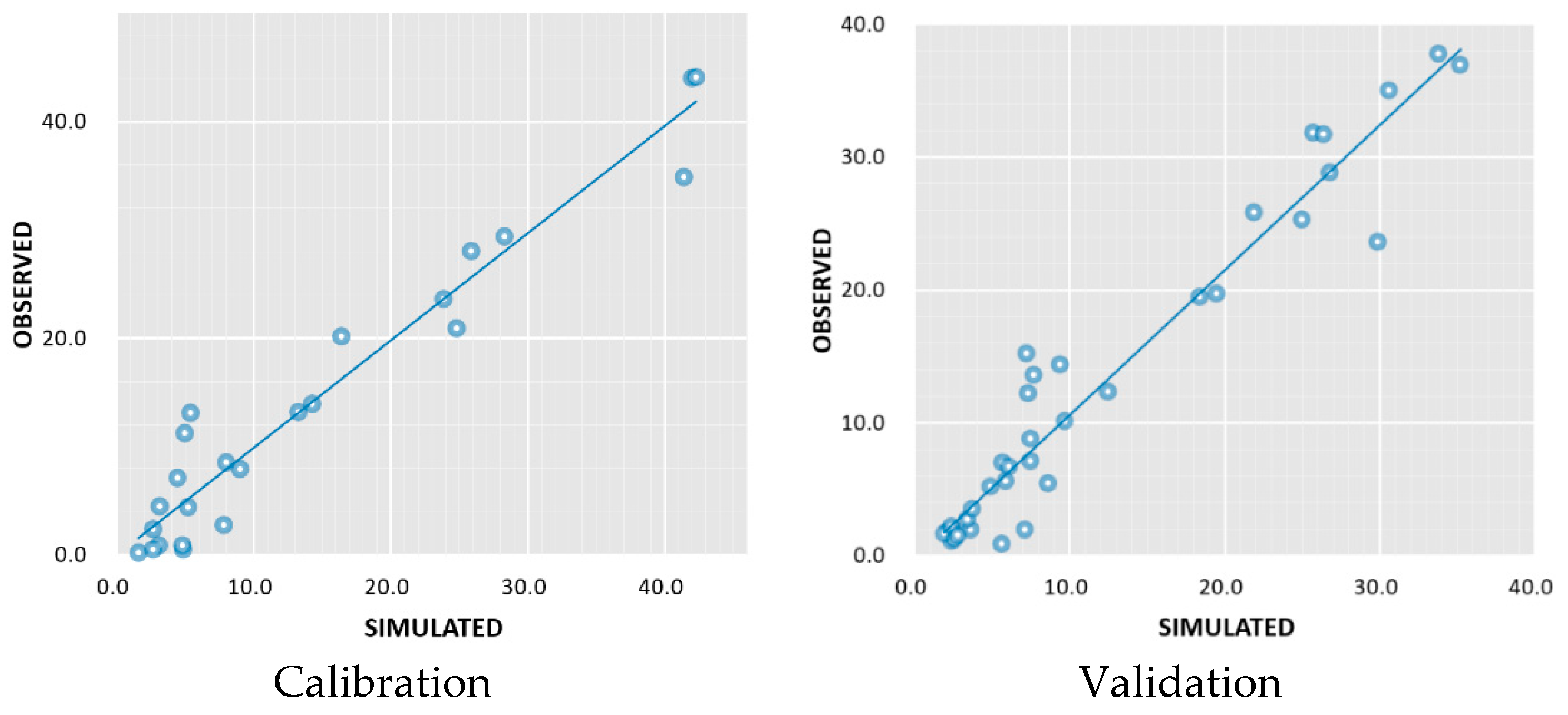
In this study, the CMADS+SWAT model was used to export the monthly runoff of the two hydrological stations (Jinghe mountain station and Hot Spring station), and the parameters were calibrated (see Figure 3, Figure 4, Figure 5 and Figure 6).
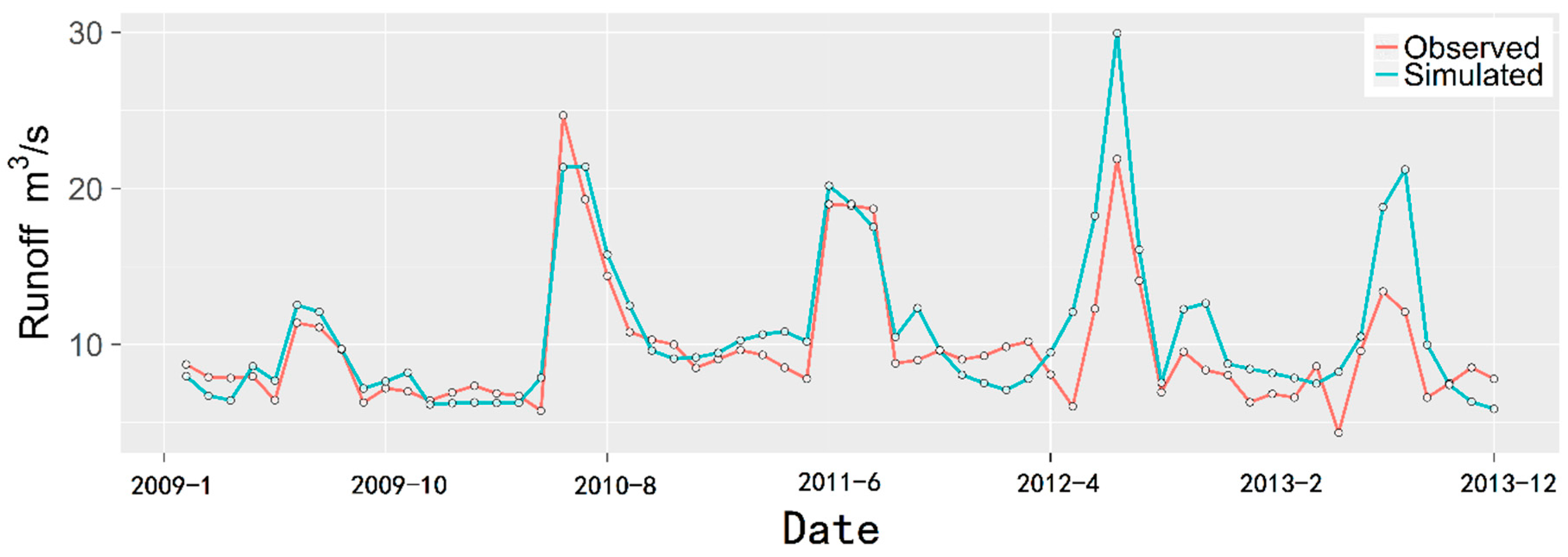
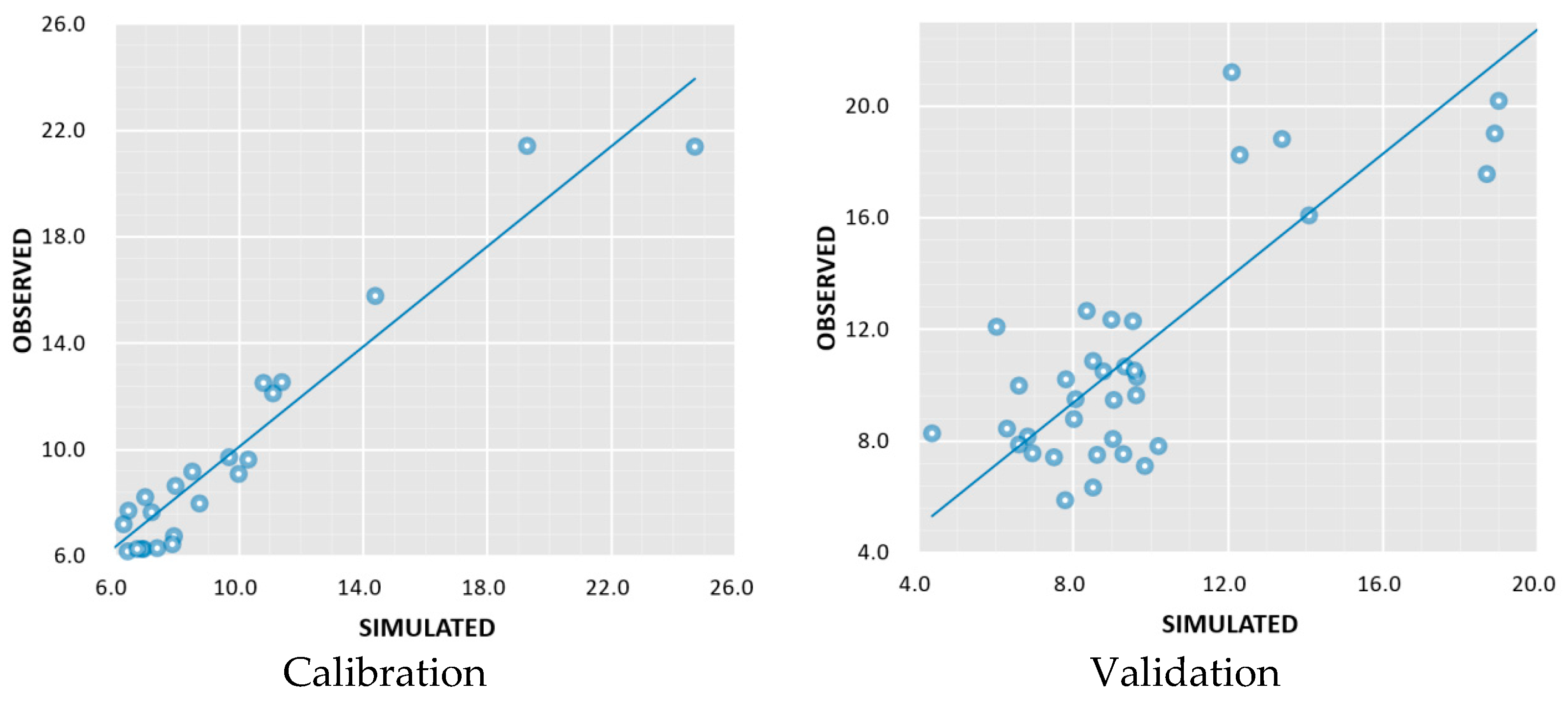
It was found that on a monthly scale, the SWAT model that is driven by CMADS has reached the satisfactory index (see Table 4) in the two control stations of the JBR. Moreover, on a monthly scale, the simulation results obtained by CMADS achieved satisfactory results (NSE = 0.939, R2 = 0.942) at the Jinghe Mountain Station (calibration period).
During the validation period, although the NSE efficiency coefficient and the R2 deterministic coefficient were slightly lower than those of the calibration period, they were overall satisfactory (NSE = 0.904, R2 = 0.934). Compared with the Jinghe mountain station, the simulation accuracy of the Hot Spring station in the calibration and the verification periods were slightly lower. The authors believe that the glacier in the upper reaches of the Hot Spring has a great influence on the simulation results of the Hot Spring station. Furthermore, in the SWAT model, the degree-day factor only considers the snowmelt factor carefully, which leads to the simulation accuracy of the river basin in the Hot Spring station to be lower than that of the Jinghe Control Station (where the glacier replenishment rate is smaller than that of the former).
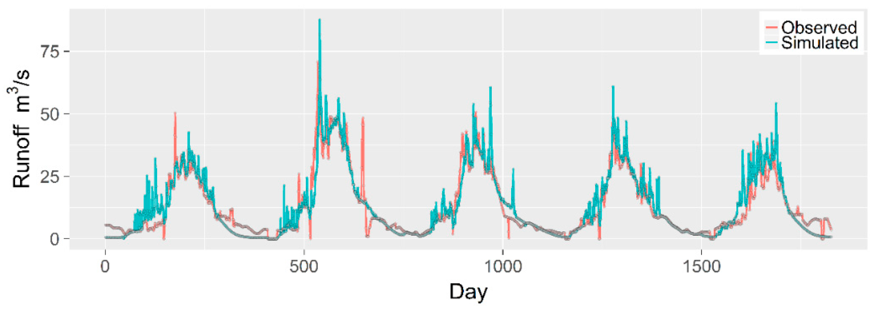
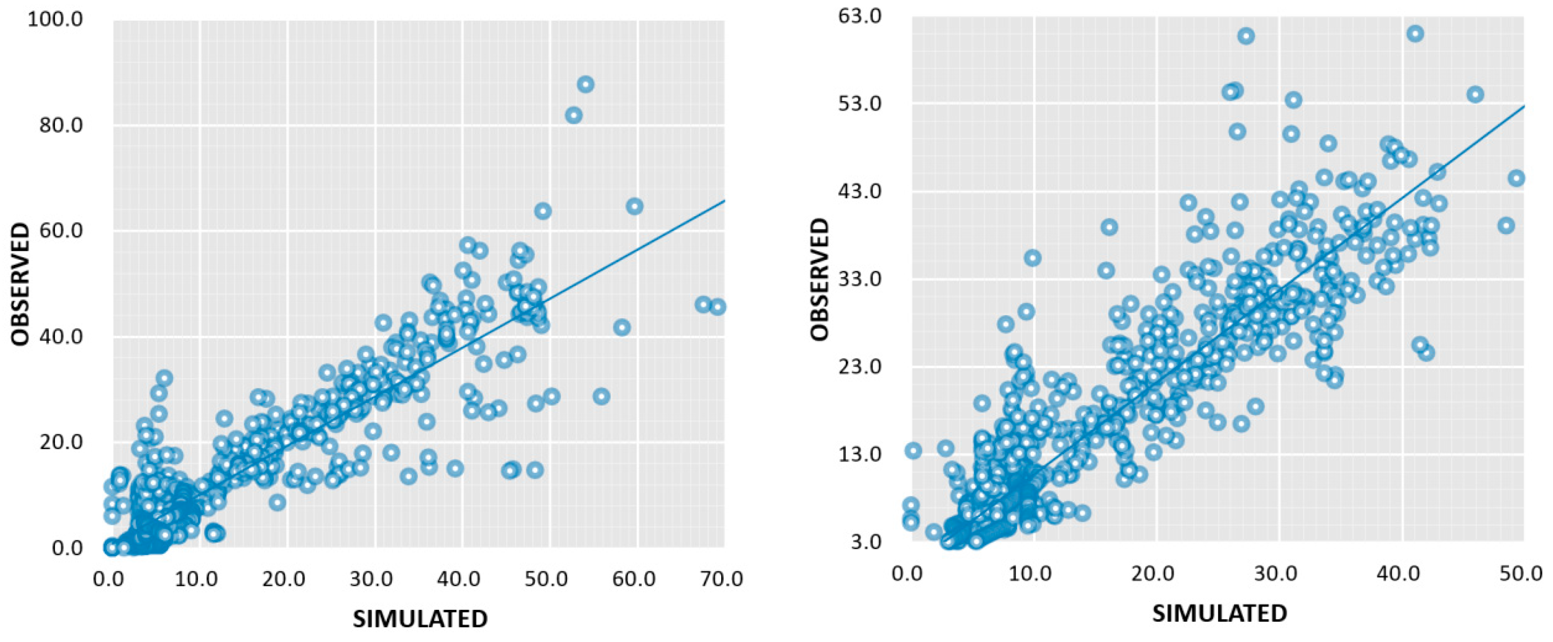
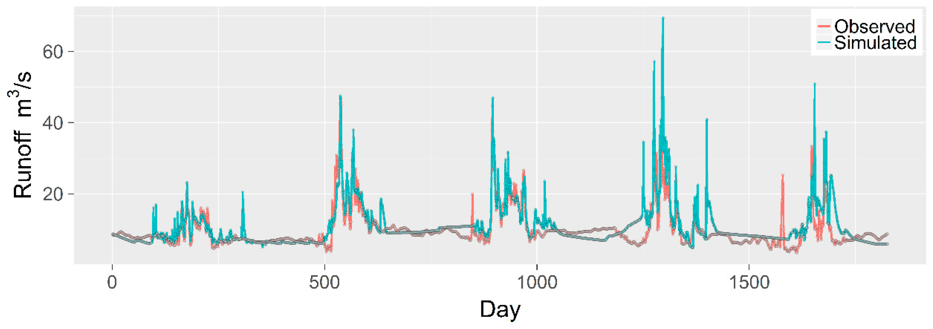
After completing the monthly scale calibration and verification, this study inputs the monthly scale optimal parameter value into the SWAT model for daily fine tuning and calibration. The results show that the SWAT model driven by the CMADS achieves acceptable results on a daily scale for the two control stations (see Figure 7, Figure 8, Figure 9 and Figure 10, and Table 4). The runoff simulation results of the SWAT model driven by the CMADS demonstrate good consistency in the daily hydrological graphs of the two sub-watersheds.
In the calibration period, the results for the Jinghe Mountain Station (NSE = 0.801, R2 = 0.815) were similar to those of the Hot Spring Station (NSE = 0.0.796, R2 = 0.791), and the results were simulated on the basis of the daily simulation driven by the CMADS. During the model’s validation period, although the SWAT model was acceptable at both sites, the simulation results (NSE = 0.851, R2 = 0.796) from the model in the Jinghe mountain Station were superior to those of the Hot Spring Station (NSE = 0.526, R2 = 0.592).
4.2. Spatial and Temporal Distribution Variation of Hydrological Processes
Since the SWAT model have been localized to the JBR and obtained satisfactory results, in order to analyze the ability of the CMADS+SWAT model to simulate the spatial and temporal evolution of the soil moisture and snowmelt variables from time and space perspectives, and to quantitatively analyze the response between the components, this study uses the Jinghe sub-basin as the main object of analysis object, and extracts the relationship between the multiple elements.
4.2.1. Response of Snowmelt Process and Soil Moisture
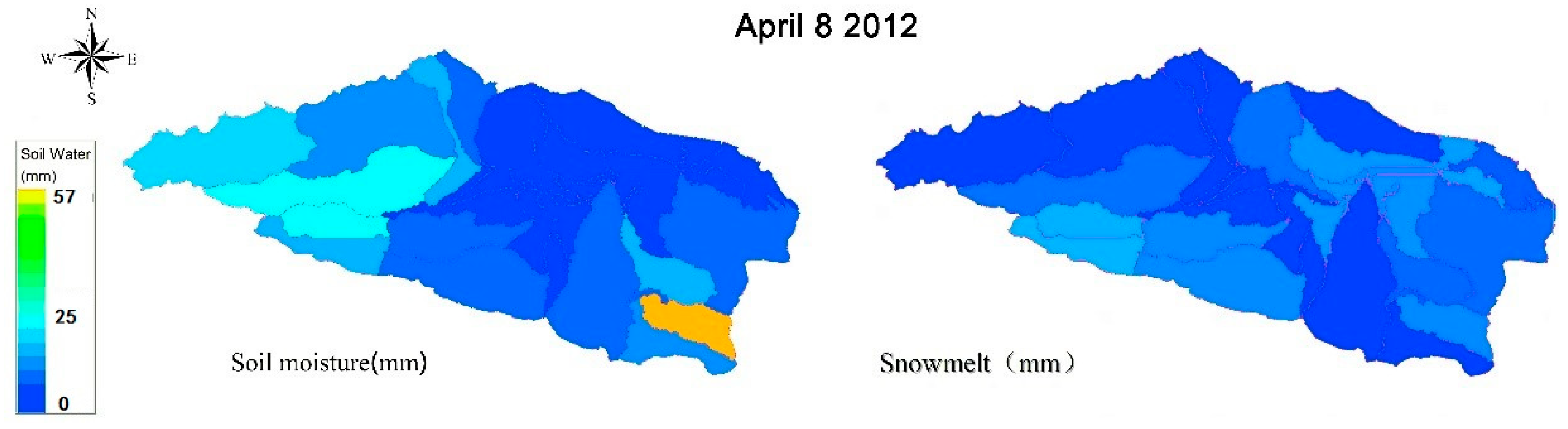
In order to study the effect of snowmelt on the soil moisture, this part of the study extracted the spatial variation of the soil moisture and the corresponding snowmelt (Figure 11) of the whole river basin on 8 April 2012. The left figure displays the soil moisture distribution, whilst the right one shows the corresponding time of the snowmelt’s spatial distribution. In order to analyze the relationship between the various surface components in the basin quantitatively, this study also extracted the time series of various surface components (including the soil moisture, potential evapotranspiration, precipitation and snowmelt) in the river basin (see Figure 12).
Through the distribution of the soil moisture throughout the JBR on 8 April 2012, it was found that the soil moisture in the entire basin was in a wet state on that day (see Figure 14A). Furthermore, where the Hot Spring station controls the sub-watershed soil, its moisture was between 18 mm and 20 mm, whereas the soil moisture of the Jinghe Control Station and its nearby sub-basin reached nearly 57 mm. It was also found that on 8 April 2012, by analyzing the spatial distribution of the corresponding snowmelt in the basin (Figure 14A1), there was a large snowmelt in the JBR. Moreover, the main area where snowmelt occurred was just the northern slope of the western Tianshan Mountains, which experiences a huge snow cover for 3-4 months in a year. In order to analyze the magnitude of snowmelt and soil moisture in the JBR quantitatively, and to analyze the direct response relationship, this study carried out a time series analysis of the soil moisture and snowmelt in a single sub-basin that is under the control of the Jinghe Hydrological Station (Jinghe Mountain Station).
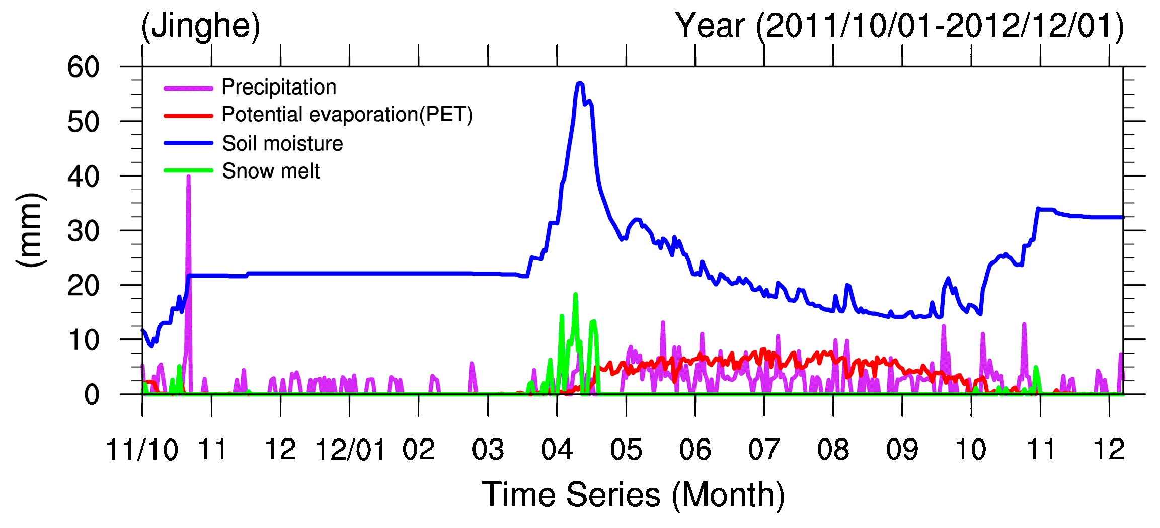
Figure 12 shows the various types of surface or near-surface components (i.e., potential evapotranspiration, soil moisture, precipitation and amount of snowmelt) in the river basin. It was found that the snow melting phenomenon began to occur in the middle of March 2012, and the snowmelt phenomenon appeared on 8 April 2012. The snowfall of the Jinghe was 18 mm/day and the soil moisture in the natural sub-basin of the Jinghe Control Station also reached a high level (about 56 mm) during this period. The analysis also found that the most important contributor of the soil moisture’s increase when the snow fell was the snow itself, with only a small amount coming from precipitation. In addition, the soil moisture was in inverse proportion to the potential evaporation values.
4.2.2. Response of Precipitation and Soil Moisture
This paper has analyzed the Jinghe sub-basin in the JBR, and focused on the influence of snowmelt on the soil moisture. However, in addition to the snow melt phenomenon, the impact of precipitation on the soil moisture cannot be ignored. This section analyzes the effects of precipitation on the soil moisture from summer to autumn, since the precipitation of snowfall in early spring has been analyzed. As the soil moisture in the study area will fluctuate during the long period of time between the snow melting period and September, and the sudden rise of the soil during the middle and late period of October will remain constant, the authors will compare the above two stages of precipitation and soil moisture using a response analysis of both time and space extraction; this will also serve to verify the changes of other variables (such as permafrost and snow depth) during the change of soil moisture in the Jinghe Mountain Station. This study also extracted the observation data of ice and snow (between 2010 and 2011) (Figure 13A,B,A1,B1).
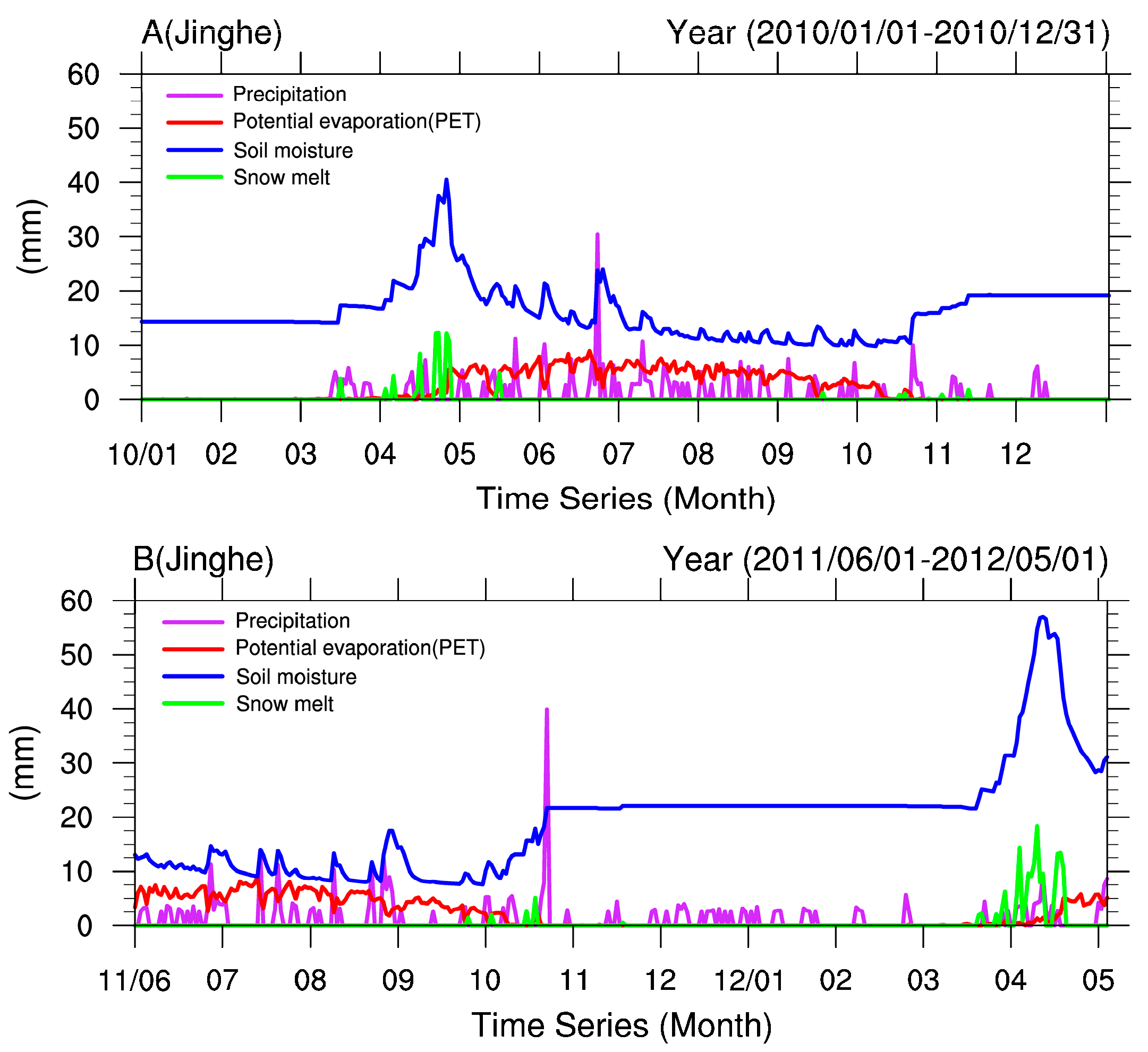
Figure 13A,B1 shows the spatial distribution of the soil moisture and precipitation in the JBR during the days of 22 June 2010 and 21 October 2011. Figure 13A shows the distribution of the soil moisture in the Bo River Basin on 22 June, 10 June, and Figure 13A1 shows the distribution of precipitation in the corresponding watershed. The results show that the soil moisture in the control basin was 24.8 mm, and the precipitation in the control area of the Jinghe Mountain Station was 30.1mm. The results also show that the increase of precipitation during the day led to the rapid increase of soil moisture in a short period. A similar situation also occurred in 2011, as shown in Figure 13A1, for the spatial distribution of soil moisture on 21 October. Figure 13B1 shows the distribution of precipitation over the entire basin in the corresponding period. It was found that the soil moisture in the sub-basin of the Jinghe mountain station and Hot Spring station is substantial, with 22 mm and 18mm, repectively. The analysis also found that, while the soil moisture in the basin reached a high level in the same period, the precipitation occurred in the whole sub-basin of the Jinghe and Bortala Rivers. In order to accurately verify the response relationship between the soil moisture and precipitation in order of magnitude, this study extracted other surface components (i.e., potential evapotranspiration, soil moisture, precipitation and snow melt) of the Jinghe mountain station (2011–2012) that corresponded with the other results (Figure 14AB).
The results show that the precipitation in the basin was close to 30 mm on 22 June 2010, and the soil moisture also reached 24.8 mm (Figure 14A), corresponding to the above spatial distribution. On 21 October 2011, the precipitation in the sub-basin of the Jinghe Yamaguchi Control Station reached nearly 40 mm. At the same time, the soil moisture value in the sub-basin also climbed to about 22 mm and remained constant thereafter (Figure 14B). The rapid increase of the soil moisture at the above two streams of the Jinghe Mountain station indicates that the precipitation in the late autumn in the Jinghe Mountain sub-basin plays an important role in the later changes of the soil moisture.
The overall change of the soil moisture from the annual circulation’s perspective was analyzed. In the study area, the snow depth analyzed in the basin is from the third to fourth month of the research. The snow depth in the basin has experienced the rising and falling processes, and is close to 0 at the end of the snow melting. This is consistent with the snow depth observations extracted from the Jinghe Station (Figure 15A,C). In the later period, the climatic temperature of the study area rapidly increased, and as the air temperature is higher in this period, the frozen soil melts (Figure 15B,D). The soil evaporation also increased and accelerated the evaporation of soil water, which influenced the soil moisture’s trend at this time. Ten months after the snow arrived, due to the cold and humid air flow over a wide range of precipitation (snow), the soil water content in the river basin increased significantly, which, as well as the cold air, is also caused by a significant reduction in evaporation. At this point, the soil liquid water content freezes (from November to December each year) and frozen soil is produced. Additionally, until the melting season occurs in the following year, when the frozen soil melting phenomenon occurs once again, part of the permafrost will be converted into soil liquid water.
In summary, the soil moisture in the basin will reach its first high level from March to April each year, mainly due to the snowmelt in the basin. After the end of the snowmelt period, the increase in precipitation and air temperature, as well as other phenomena, will lead to a trend in the soil temperature fluctuation. In mid-October the cold air arrives, leading to a large amount of precipitation (snow), and eventually turning the water in the soil into a frozen state. During the snow melt period in the following year, the soil liquid water increases again until the end of the snowmelt period.
Most researchers in China used traditional meteorological observatories with relatively scarce distribution when they studied the Western basin in China in the past. Similar studies have shown that scarce meteorological observatories do not represent the real underlying surface [48], resulting in greater uncertainty in meteorological inputs and the uncertainty of model output is affected [33]. For example, some researchers were able to obtain only one weather station on the north slope of the Tianshan mountains for surface analysis of Juntanghu watershed [29]. In addition, the mode output of climate change scenario prediction will be very unreliable when traditional weather stations are unable to effectively calibrate the SWAT model [1,32,34]; some scholars have realized that the western region of China needs to use the re-analysis data set to make up for the lack of data to drive SWAT. However, these researchers did not achieve good results by directly using reanalysis-data-driven SWAT without local correction. This is because most meteorological reanalysis data did not use automatic stations in China for correction, and cannot accurately reflect the intensity and frequency of the underlying surface in real weather [16]. Taking central Asia as an example, some scholars believe that an improper setting of climate simulation may lead to errors in simulation of ground climate field in regions with complex terrain and obvious spatial differences of meteorological elements [28]. For example, when the CFSR is used to drive the SWAT model, it can be found that the CFSR precipitation is overestimated in summer, resulting in overestimated runoff [44,45,46].
Different from other studies, CMADS driving SWAT model was selected in this study, and important surface process components (such as soil temperature, soil moisture, snowmelt, etc.) were obtained. Under the condition of SWAT calibration, we believed that these surface processes could be trusted. In the future, in order to reduce the output uncertainty of the SWAT model and obtain the best simulation results, we will focus on adjusting the parameterized scheme based on CMADS+SWAT mode. At the same time, the real-time data (CMADS-WRF) can be further used to drive the SWAT model, providing early warning for the western region of China to minimize local environmental pollution and property loss.
5. Conclusions
Based on the typical analysis and verification area of the JBR in Xinjiang, the China Meteorological Assimilation Driving Datasets for the SWAT model (CMADS) was selected to drive the SWAT model. The spatiotemporal distribution of soil moisture, snowmelt, evaporation and precipitation was analyzed within this area to verify the availability of the CMADS in western China.
The study found that:
- (1)
- The SWAT model was well calibrated by the CMADS. On the monthly scale, the performance of the SWAT model reached a satisfactory level in two control stations (Hot Spring and Jinghe Mountain) within the JBR (see Table 4). During the validation period, the simulation result (NSE = 0.851, R2 = 0.796) of the model at Jinghe Station was better than that in Hot Spring station (NSE = 0.526, R2 = 0.592). After localization the SWAT model, the daily simulated runoff (year 2012) was extracted in the study area, and we found that the SWAT model reproduced the runoff perfectly in year 2012.
- (2)
- From the perspective of time and space: During the snowmelt period, the main source of the soil moisture increase in the JBR is snowmelt, while only a small amount comes from precipitation; soil moisture and potential evaporation value show an inverse phenomenon; precipitation formed at the end of autumn in the sub-basin controlled by the Jinghe Mountain has played an important role in the later change of soil moisture. Soil moisture in the basin reaches its first high level in March-April each year, which is mainly caused by snow melting in the basin. After the snowmelt period, the soil temperature fluctuates upward and downward due to the increase of precipitation and the warming of air temperature. Until mid-October, the cold air transits and produces heavy precipitation (snow) and eventually converts the soil water into frozen soil. The next year, when the snowmelt period arrives, the liquid water of the soil increases again until the end of the snowmelt period.
- (3)
- The overall research shows that the CMADS can localization the SWAT model perfectly and and can effectively calculate other surface processes (Soil moisture, snowmelt, etc.), We believe that CMADS will provide an important data base for the lack of sites in western China, and provide more raw material for scientific discovery.
Author Contributions
Y.W. were primarily accountable for data collection and design and coordination of the study. Y.L. were responsible for data analysis and writing of the paper. J.Z. and M.Y. were responsible for results presentation.
Funding
The research was founded by the National Science Foundation of China (41701076, 51709271, 41661040), the Young Elite Scientists Sponsorship Program by CAST (2017QNRC001) and the Xinjiang Youth Science and Technology Innovation Talents Training Project (2015), (2017).
Conflicts of Interest
The authors declare no conflict of interest.
References
- Meng, X.; Wang, H.; Lei, X.; Cai, S.; Wu, H.; Ji, X.; Wang, J. Hydrological Modeling in the Manas River Basin Using Soil and Water Assessment Tool Driven by CMADS. Teh. Vjesn. 2017, 24, 525–534. [Google Scholar]
- Berg, A.A.; Famiglietti, J.S.; Walker, J.P.; Houser, P.R. Impact of bias correction to reanalysis products on simulations of North American soil moisture and hydrological fluxes. J. Geophys. Res. Atmos. 2003, 108, 4490. [Google Scholar] [CrossRef]
- Maurer, E.P.; Wood, A.W.; Adam, J.C.; Lettenmaier, D.P. A long-term hydrologically based dataset of LAND SURFACE FLUX and states for the conterminous United States. J. Clim. 2002, 15, 3237–3251. [Google Scholar] [CrossRef]
- Fekete, B.M.; Vörösmarty, C.J.; Roads, J.O.; Willmott, C.J. Uncertainties in precipitation and their impacts on runoff estimates. J. Clim. 2004, 17, 294–304. [Google Scholar] [CrossRef]
- Sheffield, J.; Ziegler, A.D.; Wood, E.F.; Chen, Y. Correction of the high-latitude rain day anomaly in the NCEP-NCAR reanalysis for land surface hydrological modeling. J. Clim. 2004, 17, 294–304. [Google Scholar] [CrossRef]
- Monteith, J.L. Evaporation and the environment. In The State and Movement of Water in Living Organisms, 19th Symposium of the Society for Experimental Biology; Cambridge University Press: Swansea, UK, 1965; pp. 205–234. [Google Scholar]
- Allen, R.G. A Penman for all seasons. J. Irrig. Drain. Eng. 1986, 112, 348–368. [Google Scholar] [CrossRef]
- Allen, R.G.; Jensen, M.E.; Wright, J.L.; Burman, R.D. Operational estimates of reference evapotranspiration. Agron. J. 1989, 81, 650–662. [Google Scholar] [CrossRef]
- Priestley, C.H.B.; Taylor, R.D. On the assessment of surface heat flux and evaporation using large-scale parameters. Mon. Weather Rev. 1972, 100, 81–92. [Google Scholar] [CrossRef]
- Hargreaves, G.H. Moisture availability and crop production. Trans. ASAE 1975, 18, 980–984. [Google Scholar] [CrossRef]
- Hargreaves, G.H.; Samani, Z.A. Reference crop evapotranspiration from temperature. Appl. Eng. Agric. 1985, 1, 96–99. [Google Scholar] [CrossRef]
- Hargreaves, G.H.; Samani, Z.A. Estimating potential evapotranspiration. J. Irrig. Drain. Eng. 1982, 108, 225–230. [Google Scholar]
- Leo Hargreaves, G.; Hargreaves, G.H.; Paul Riley, J. Agricultural benefits for Senegal River Basin. J. Irrig. Drain. Eng. 1985, 111, 113–124. [Google Scholar] [CrossRef]
- Abbaspour, K.C.; Vejdani, M.; Haghighat, S. SWAT-CUP calibration and uncertainty programs for SWAT. In Proceedings of the MODSIM 2007 International Congress on Modelling and Simulation, Christenchurch, New Zealand, 10–13 December 2007; pp. 1596–1602. [Google Scholar]
- Nash, J.E.; Sutcliffe, J.V. River Flow Forecasting through conceptual models part 1—A discussion of principles. J. Hydrol. 1970, 10, 282–290. [Google Scholar] [CrossRef]
- Meng, X.; Wang, H.; Cai, S.; Zhang, X.; Leng, G.; Lei, X.; Shi, C.; Liu, S.; Shang, Y. The China Meteorological Assimilation Driving Datasets for the SWAT Model (CMADS) Application in China: A Case Study in Heihe River Basin. Preprints. 2016. [Google Scholar] [CrossRef]
- Kalnay, E.; Kanamitsu, M.; Kistler, R.; Collins, W.; Deaven, D.; Gandin, L.; Iredell, M.; Saha, S.; White, G.; Woollen, J.; et al. The NCEP/NCAR 40-year reanalysis project. Bull. Amer. Meteorol. Soc. 1996, 77, 437–472. [Google Scholar] [CrossRef]
- Kanamitsu, M.; Ebisuzaki, W.; Woollen, J.; Yang, S.-K.; Hnilo, J.J.; Fiorino, M.; Potter, G.L. NCEP-DOE AMIP-II Reanalysis (R-2). Bull. Am. Meteorol. Soc. 2002, 83, 1631–1644. [Google Scholar] [CrossRef]
- Uppala, S.M.; Kållberg, P.M.; Simmons, A.J.; Andrae, U.; Da Costa Bechtold, V.; Fiorino, M.; Gibson, J.K.; Haseler, J.; Hernandez, A.; Kelly, G.A.; et al. The ERA-40 re-analysis. Q. J. R. Meteorol. Soc. 2005, 131, 2961–3012. [Google Scholar] [CrossRef] [Green Version]
- Onogi, K.; Tsutsui, J.; Koide, H.; Sakamoto, M.; Kobayashi, S.; Hatsushika, H.; Matsumoto, T.; Yamazaki, N.; Kamahori, H.; Takahashi, K.; et al. The JRA-25 Reanalysis. J. Meteorol. Soc. Jpn. Ser. II 2007, 85, 369–432. [Google Scholar] [CrossRef] [Green Version]
- Zhao, T.; Ailikun; Feng, J. An intercomparison between NCEP reanalysis and observed data over China. Clim. Environ. Res. 2004, 9, 278–294. [Google Scholar]
- Zhao, T.; Fu, C. Applicability evaluation of surface air temperature form several reanalysis dataset in China. Plateau Meteorol. 2009, 28, 595–607. [Google Scholar]
- Zhao, T.; Fu, C. Preliminary comparison and analysis between ERA-40, NCEP-2 reanalysis and observations over Chnia. Clim. Environ. Res. 2006, 11, 15–33. [Google Scholar]
- Shi, X.H.; Xu, X.D.; Xie, L.A. Reliability analyses of anomalies of NCEP/NCAR reanalysis wind speed and surface temperature in climate change research in China. Acta Meteorol. Sin. 2006, 64, 709–722. [Google Scholar]
- Liu, S.; Yao, X.; Guo, W.; Xu, J.; Shangguan, D.; Wei, J.; Bao, W.; Wu, L. The contemporary glaciers in China based on the Second Chinese Glacier Inventory. Acta Geogr. Sin. 2015, 70, 3–16. [Google Scholar]
- Meng, X.; Wang, H.; Shi, C.; Wu, Y.; Ji, X. Establishment and Evaluation of the China Meteorological Assimilation Driving Datasets for the SWAT Model (CMADS). Water 2018, 10, 1555. [Google Scholar] [CrossRef]
- Meng, X.; Wang, H.; Wu, Y.; Long, A.; Wang, J.; Shi, C.; Ji, X. Investigating spatiotemporal changes of the land-surface processes in Xinjiang using high-resolution CLM3.5 and CLDAS: Soil temperature. Sci. Rep. 2017, 7, 13286. [Google Scholar] [CrossRef] [PubMed] [Green Version]
- Meng, X.; Wang, H. Significance of the China Meteorological Assimilation Driving Datasets for the SWAT Model (CMADS) of East Asia. Water 2017, 9, 765. [Google Scholar] [CrossRef]
- Shi, C.X.; Xie, Z.H.; Qian, H.; Liang, M.L.; Yang, X.C. China land soil moisture EnKF data assimilation based on satellite remote sensing data. Sci. China Earth Sci. 2011, 54, 1430–1440. [Google Scholar] [CrossRef]
- Dong, N.; Yang, M.; Meng, X.; Liu, X.; Wang, Z.; Wang, H.; Yang, C. CMADS-Driven Simulation and Analysis of Reservoir Impacts on the Streamflow with a Simple Statistical Approach. Water 2018, 11, 178. [Google Scholar] [CrossRef]
- Stamnes, K.; Tsay, S.C.; Wiscombe, W.; Jayaweera, K. Numerically stable algorithm for discrete-ordinate-method radiative transfer in multiple scattering and emitting layered media. Appl. Opt. 1988, 27, 2502–2509. [Google Scholar] [CrossRef] [PubMed]
- Meng, X.-Y.; Yu, D.-L.; Liu, Z.-H. Energy balance-based SWAT model to simulate the mountain snowmelt and runoff—Taking the application in Juntanghu watershed (China) as an Example. J. Mt. Sci. 2015, 12, 368–381. [Google Scholar] [CrossRef]
- Wang, Y.J.; Meng, X.Y.; Liu, Z.H. Snowmelt Runoff Analysis under Generated Climate Change Scenarios for the Juntanghu River Basin, in Xinjiang, China. Tecnol. Cienc. Agua 2017, 7, 41–54. [Google Scholar]
- Meng, X.; Long, A.; Wu, Y.; Yin, G.; Wang, H.; Ji, X. Simulation and spatiotemporal pattern of air temperature and precipitation in Eastern Central Asia using RegCM. Sci. Rep. 2018, 8, 3639. [Google Scholar] [CrossRef] [PubMed] [Green Version]
- Meng, X.; Sun, Z.; Zhao, H.; Ji, X.; Wang, H.; Xue, L.; Wu, H.; Zhu, Y. Spring Flood Forecasting Based on the WRF-TSRM Mode. Teh. Vjesn. 2018, 1, 141–151. [Google Scholar]
- Zhao, F.; Wu, Y.; Qiu, L.; Sun, Y.; Sun, L. Parameter Uncertainty Analysis of the SWAT Model in a Mountain-Loess Transitional Watershed on the Chinese Loess Plateau. Water 2018, 10, 690. [Google Scholar] [CrossRef]
- Vu, T.T.; Li, L.; Jun, K.S. Evaluation of Multi-Satellite Precipitation Products for Streamflow Simulations: A Case Study for the Han River Basin in the Korean Peninsula, East Asia. Water 2018, 10, 642. [Google Scholar] [CrossRef]
- Liu, J.; Shanguan, D.; Liu, S.; Ding, Y. Evaluation and Hydrological Simulation of CMADS and CFSR Reanalysis Datasets in the Qinghai-Tibet Plateau. Water 2018, 10, 513. [Google Scholar] [CrossRef]
- Cao, Y.; Zhang, J.; Yang, M.; Lei, X. Application of SWAT Model with CMADS Data to Estimate Hydrological Elements and Parameter Uncertainty Based on SUFI-2 Algorithm in the Lijiang River Basin, China. Water 2018, 10, 742. [Google Scholar] [CrossRef]
- Shao, G.; Guan, Y.; Zhang, D.; Yu, B.; Zhu, J. The Impacts of Climate Variability and Land Use Change on Streamflow in the Hailiutu River Basin. Water 2018, 10, 814. [Google Scholar] [CrossRef]
- Zhou, S.; Wang, Y.; Chang, J.; Guo, A.; Li, Z. Investigating the Dynamic Influence of Hydrological Model Parameters on Runoff Simulation Using Sequential Uncertainty Fitting-2-Based Multilevel-Factorial-Analysis Method. Water 2018, 10, 1177. [Google Scholar] [CrossRef]
- Gao, X.; Zhu, Q.; Yang, Z.; Wang, H. Evaluation and Hydrological Application of CMADS against TRMM 3B42V7, PERSIANN-CDR, NCEP-CFSR, and Gauge-Based Datasets in Xiang River Basin of China. Water 2018, 10, 1225. [Google Scholar] [CrossRef]
- Tian, Y.; Zhang, K.; Xu, Y.-P.; Gao, X.; Wang, J. Evaluation of Potential Evapotranspiration Based on CMADS Reanalysis Dataset over China. Water 2018, 10, 1126. [Google Scholar] [CrossRef]
- Qin, G.; Liu, J.; Wang, T.; Xu, S.; Su, G. An Integrated Methodology to Analyze the Total Nitrogen Accumulation in a DrinkingWater Reservoir Based on the SWAT Model Driven by CMADS: A Case Study of the Biliuhe Reservoir in Northeast China. Water. 2018, 10, 1535. [Google Scholar] [CrossRef]
- Ebita, A.; Kobayashi, S.; Ota, Y.; Moriya, M.; Kumabe, R.; Onogi, K.; Harada, Y.; Yasui, S.; Miyaoka, K.; Takahashi, K.; et al. The Japanese 55-Year Reanalysis “JRA-55”: An interim report. SOLA 2011, 7, 149–152. [Google Scholar] [CrossRef]
- Dee, D.P.; Uppala, S.M.; Simmons, A.J.; Berrisford, P.; Poli, P.; Kobayashi, S.; Andrae, U.; Balmaseda, M.A.; Balsamo, G.; Bauer, P.; et al. The ERA—Interim reanalysis: Configuration and performance of the data assimilation system. Q. J. R. Meteor. Soc. 2011, 137, 553–597. [Google Scholar] [CrossRef]
- Saha, S.; Moorthi, S.; Pan, H.L.; Wu, X.; Wang, J.; Nadiga, S.; Tripp, P.; Kistler, R.; Woollen, J.; Behringer, D.; et al. The NCEP climate forecast system reanalysis. Bull. Am. Meteorol. Soc. 2010, 91, 1015–1057. [Google Scholar] [CrossRef]
- Rienecker, M.M.; Suarez, M.J.; Gelaro, R.; Todling, R.; Bacmeister, J.; Liu, E.; Bosilovich, M.G.; Schubert, S.D.; Takacs, L.; Kim, G.; et al. MERRA: NASA’s modern-era retrospective analysis for research and applications. J. Clim. 2011, 24, 3624–3648. [Google Scholar] [CrossRef]
- Li, L.; Bai, L.; Yao, Y.; Yang, Q.; Zhao, X. Patterns of climate change in Xinjiang projected by IPCC SRES. J. Resour. Ecol. 2013, 4, 27–36. [Google Scholar]
- Lioubimtseva, E.; Cole, R. Uncertainties of climate change in arid environments of Central Asia. Rev. Fish. Sci. 2006, 14, 29–49. [Google Scholar] [CrossRef]
- Xu, Y.; Gao, X.; Shen, Y.; Xu, C.; Shi, Y.; Giorgi, F. A daily temperature dataset over China and its application in validating a RCM simulation. Adv. Atmos. Sci. 2009, 26, 763–772. [Google Scholar] [CrossRef] [Green Version]
- Santhi, C.; Arnold, J.G.; Williams, J.R.; Hauck, L.M.; Dugas, W.A. Application of a watershed model to evaluate management efforts on point and nonpoint source pollution. Trans. ASAE 2011, 44, 1559–1570. [Google Scholar]
- Nafees Ahmad, H.M.; Sinclair, A.; Jamieson, R.; Madani, A.; Hebb, D.; Havard, P.; Yiridoe, E.K. Modeling sediment and nitrogen export from a rural watershed in Eastern Canada using the soil and water assessment tool. J. Environ. Qual. 2011, 40, 1182–1194. [Google Scholar] [CrossRef] [PubMed]
- Moriasi, D.N.; Arnold, J.G.; Van Liew, M.W.; Bingner, R.L.; Harmel, R.D.; Veith, T.L. Model Evaluation Guidelines for Systematic Quantification of Accuracy in Watershed Simulations. Trans. ASABE 2007, 50, 885–900. [Google Scholar] [CrossRef]
Figure 1.
Location of Jinghe and Bortala River Basins (JBR).

Figure 2.
(a) Soil classification and (b) Land usage distribution.Remarks: SWGR: Slender Wheat grass; PAST: Pasture; HAY: Hay; WETL: Wetlands-Mixed; WATR: Water; AGRL: Agricultural Land-Generic; AGRR: Agricultural Land-Row Crops; URML: Residential-Med/Low Density; UIDU: Industrial; UTRN: Transportation; FRST: Forest-Mixed; RNGE: Range-Grasses; BARO: Bare rock; DESE: Desert; SALA: Saline land; GLSN: Glacier and snow; FRSD: Forest-Deciduous; PINE: Pine; RNGB: Range-Brush; ORCD: Orchard; FRSE: Forest-Evergreen.


Figure 3.
Monthly runoff (2009–2013) of Jinghe mountain station derived from the SWAT model driven by the CMADS.
Figure 3.
Monthly runoff (2009–2013) of Jinghe mountain station derived from the SWAT model driven by the CMADS.

Figure 4.
Deterministic coefficients of the monthly observed and simulated runoff of Jinghe mountain station.
Figure 4.
Deterministic coefficients of the monthly observed and simulated runoff of Jinghe mountain station.

Figure 5.
Monthly runoff (2009–2013) of Hot Spring station derived from the SWAT model driven by the CMADS.
Figure 5.
Monthly runoff (2009–2013) of Hot Spring station derived from the SWAT model driven by the CMADS.

Figure 6.
Deterministic coefficients of the monthly observed and simulated runoff of the Hot Spring station.
Figure 6.
Deterministic coefficients of the monthly observed and simulated runoff of the Hot Spring station.

Figure 7.
Daily runoff (2009–2013) of Jinghe mountain station derived from the SWAT model driven by the CMADS.
Figure 7.
Daily runoff (2009–2013) of Jinghe mountain station derived from the SWAT model driven by the CMADS.

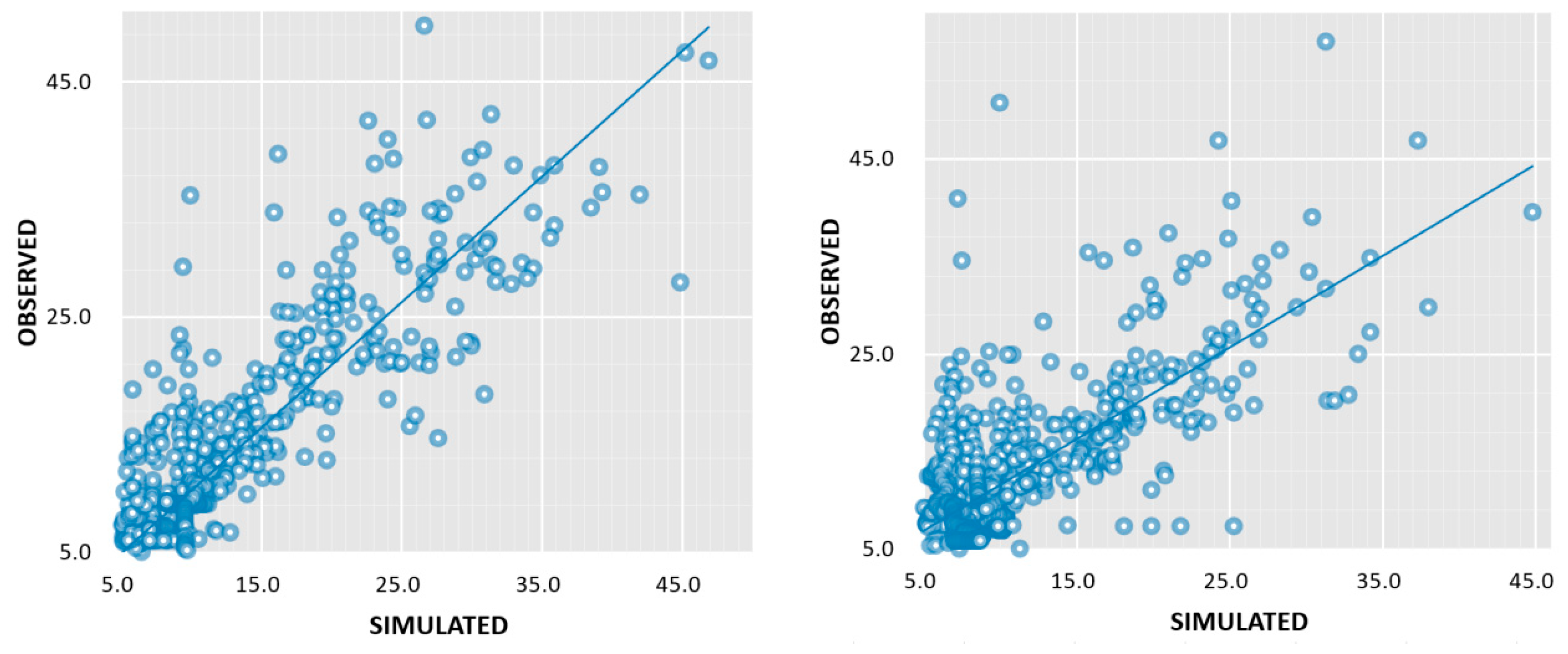
Figure 8.
Deterministic coefficients of the daily observed and simulated runoff of Jinghe mountain station.
Figure 8.
Deterministic coefficients of the daily observed and simulated runoff of Jinghe mountain station.

Figure 9.
Daily runoff (2009–2013) of Hot Spring station derived from the SWAT model driven by the CMADS.
Figure 9.
Daily runoff (2009–2013) of Hot Spring station derived from the SWAT model driven by the CMADS.

Figure 10.
Deterministic coefficients of the daily observed and simulated runoff of Hot Spring station.
Figure 10.
Deterministic coefficients of the daily observed and simulated runoff of Hot Spring station.

Figure 11.
Spatial distribution of soil moisture and snowmelt rateof the JBR.

Figure 12.
Time series of the parameters of the JBR (take the Jinghe mountain station as an example).
Figure 12.
Time series of the parameters of the JBR (take the Jinghe mountain station as an example).

Figure 13.
Correlation analysis of the soil moisture and precipitation in the JBR.

Figure 14.
Time series of the soil moisture and precipitation in the JBR (Take the Jinghe Mountain station as an example).
Figure 14.
Time series of the soil moisture and precipitation in the JBR (Take the Jinghe Mountain station as an example).

Figure 15.
Snow depth and frozen depth values in 2010 and 2011 from the Jinghe Control Station.


Table 1.
The CMADS information.
| Dataset | CMADS Serial Dataset |
|---|---|
| Elements provided | Daily maximum/minimum temperature, relative humidity, wind speed, precipitation, solar radiation |
| Spatial scale of dataset | 0–65° N, 60°–160° E |
| Temporal scope of dataset | 37.5°–39.2° N, 98.5°–101.2° E |
| Data temporal scale | 1 January 2008–31 December 2013 |
| Data original resolution | 0.333°, 0.25°, 0.125°, 0.0625° |
| Spatial resolution | 0.25° |
| Number of CMADS sites in the study | 28 |
Table 2.
Information relating to the hydrological stations in the JBR.
| Station Name | Latitude | Longitude | Altitude(m) | Data Time (Year) |
|---|---|---|---|---|
| Hot Spring | 44°59′ | 81°02′ | 1310 | 2009-2013 |
| Jinghe Mountain | 44°22′ | 82°55′ | 620 | 2009-2013 |
Table 3.
The final values of the SWAT model’s parameters.
| Parameter Names | Parameter Definitions | Parameters |
|---|---|---|
| Final Values | ||
| CN2.mgt | SCS runoff curve values | 34 |
| ALPHA_BF.gw | Baseflow α factor | 0.453 |
| GW_DELAY.gw | Aquiclude replenish delay time (days) | 42 |
| GWQMN.gw | Water level threshold for shallow aquifers when groundwater is imported into the main river course | 8.5 |
| GW_REVAP.gw | Groundwater re-evaporation coefficient | 0.03 |
| ESCO.hru | Soil evaporation replenish coefficient | 1.008 |
| CH_L(1).rte | Manning value of the main water course | 94.174 |
| CH_K1.rte | River course effective infiltration coefficient | 60.302 |
| ALPHA_BNK.rte | Baseflow water recession coefficient | 0.45 |
| SFTMP | Average temperature on snowmelt day (°C) | 4.8 |
| PLAPS | Lapse rate of precipitation day (mm/km) | 44.5 |
| SMFMN | Snowmelt factor on 21 December (mm/day-°C) | 9.407 |
| SMFMX | Snowmelt factor on June 21 | 0.1302 |
| TLAPS | Temperature lapse rate (°C/km) | −4.3039 |
Table 4.
The assessment under a monthly and daily scale simulated by the CMADS+SWAT model.
| Jinghe Mountain Station | Hot Spring Station | ||||||
|---|---|---|---|---|---|---|---|
| NSE | CP R2 | VP NSE | VP R2 | CP NSE | CP R2 | VP NSE | VP R2 |
| Month | 0.939 | 0.942 | 0.904 | 0.934 | 0.917 | 0.914 | 0.659 |
| Day | 0.801 | 0.815 | 0.802 | 0.851 | 0.796 | 0.791 | 0.526 |
Note: CP represents Calibration Period, VP represents Verification Period.
© 2019 by the authors. Licensee MDPI, Basel, Switzerland. This article is an open access article distributed under the terms and conditions of the Creative Commons Attribution (CC BY) license (http://creativecommons.org/licenses/by/4.0/).
Share and Cite
MDPI and ACS Style
Li, Y.; Wang, Y.; Zheng, J.; Yang, M. Investigating Spatial and Temporal Variation of Hydrological Processes in Western China Driven by CMADS. Water 2019, 11, 435. https://doi.org/10.3390/w11030435
AMA Style
Li Y, Wang Y, Zheng J, Yang M. Investigating Spatial and Temporal Variation of Hydrological Processes in Western China Driven by CMADS. Water. 2019; 11(3):435. https://doi.org/10.3390/w11030435
Chicago/Turabian StyleLi, Yun, Yuejian Wang, Jianghua Zheng, and Mingxiang Yang. 2019. "Investigating Spatial and Temporal Variation of Hydrological Processes in Western China Driven by CMADS" Water 11, no. 3: 435. https://doi.org/10.3390/w11030435
Note that from the first issue of 2016, this journal uses article numbers instead of page numbers. See further details here.