Modelling the Impact on Root Water Uptake and Solute Return Flow of Different Drip Irrigation Regimes with Brackish Water

Abstract

Water scarcity and quality degradation represent real threats to economic, social, and environmental development of arid and semi-arid regions. Drip irrigation associated to Deficit Irrigation (DI) has been investigated as a water saving technique. Yet its environmental impacts on soil and groundwater need to be gone into in depth especially when using brackish irrigation water. Soil water content and salinity were monitored in a fully drip irrigated potato plot with brackish water (4.45 dSm⁻¹) in semi-arid Tunisia. The HYDRUS-1D model was used to investigate the effects of different irrigation regimes (deficit irrigation (T1R, 70% ETc), full irrigation (T2R, 100% ETc), and farmer’s schedule (T3R, 237% ETc) on root water uptake, root zone salinity, and solute return flows to groundwater. The simulated values of soil water content (θ) and electrical conductivity of soil solution (ECsw) were in good agreement with the observation values, as indicated by mean RMSE values (≤0.008 m³·m⁻³, and ≤0.28 dSm⁻¹ for soil water content and ECsw respectively). The results of the different simulation treatments showed that relative yield accounted for 54%, 70%, and 85.5% of the potential maximal value when both water and solute stress were considered for deficit, full. and farmer’s irrigation, respectively. Root zone salinity was the lowest and root water uptake was the same with and without solute stress for the treatment corresponding to the farmer’s irrigation schedule (273% ETc). Solute return flows reaching the groundwater were the highest for T3R after two subsequent rainfall seasons. Beyond the water efficiency of DI with brackish water, long term studies need to focus on its impact on soil and groundwater salinization risks under changing climate conditions.

1. Introduction

In arid and semi-arid regions, the growing population is facing water scarcity and climate change hazards. As drinking water is prioritized in fresh water allocation, irrigation water is often of poor quality. In Tunisia, the agricultural sector accounts for a significant share of water resources and irrigation accounts for almost 80% (about 2100 m³·y⁻¹) of the total water demand [1]. Water use efficiency and soil management are major challenges for the development and sustainability of irrigated lands [2,3]. Higher crop production and higher water use efficiency are usually achieved simultaneously with drip irrigation compared to other surface irrigation methods [4]. Drip irrigation is considered, among other irrigation methods, as a suitable technique in arid and semi-arid countries to irrigate row crops [5]. The purpose of introducing drip irrigation was to modernize the agricultural production systems and to save water in the context of water scarcity [6]. Besides, Regulated Deficit Irrigation (RDI) was proposed as an irrigation strategy to save water without reducing crop yields considerably [7,8,9]. The RDI consists of the reduction of irrigation water to predetermined levels at certain developmental crop stages. Knowing that several climate studies predicted temperature rise and rainfall depletion in arid regions [10], RDI has also been assessed as a climate change adaptation strategy [11,12,13]. However, studies recommend a better monitoring and assessment of RDI impacts on soil salinization and sodification in semi-arid areas [3]. Indeed irrigated lands are often threatened by soil degradation due to secondary salinization. Soil salinity is present in most large irrigation systems worldwide under the combined effect of aridity, poor quality of irrigation water, water logging, and agricultural practices [14]. In Tunisia, only 18% of groundwater has salinity less than 1.5 g/L, 63% of groundwater has salinity between 1.5 and 4 g/L, and 19% of groundwater (29% of shallow aquifers, 13% of deep aquifers) has salinity higher than 4 g/L, which is classified as brackish water [15]. In addition, about 50% of irrigated soils have been considered as highly sensitive to secondary salinization [16]. Salinization occurs as a consequence of salts redistribution processes related to the hydrological cycle under irrigation influence [17]. In this case, salinity becomes a factor to be taken into account in water and soil management. Soil quality monitoring must thus be made to ensure the sustainability of crop systems in irrigated areas under salinity effect. Salinity is indeed one of the main constraints responsible for soil fertility reduction leading to the loss of crop yield and thus farmer’s income drop.

Besides, soil salinization and crop yield loss, we can cite solute recycling as a major threat for the sustainability of irrigated systems. In many irrigated areas, wells are the main sources of water irrigation, especially in the dry season, which leads to extracting solutes from these wells and their re-distribution on lands. If solutes remain in the system, they will be returned to the groundwater by solute return flow from irrigation, thus increasing salinization [18,19]. Irrigation return flows are defined by the United States Geological Survey (USGS) as the irrigation water that is applied to an area and which is not consumed by evaporation or transpiration and returns to a surface stream or aquifer. Solute recycling through irrigation return flows is cited as one of the major sources of groundwater salinization [20].

Irrigation return flows were found to be dependent on the geological set of the irrigated area, soil moisture characteristic, meteorological data, crops, irrigation systems, and water table depth [21,22,23].

Combining a modeling approach with field data creates a rapid and cost effective assessment of water and salt movement under drip irrigation treatments with brackish water [24,25]. Models can also be helpful tools for designing, testing and implementing soil, water, and crop management practices that minimize soil and water contamination [26]. Among many simulation models, the numerical model HYDRUS-1D [27] is considered an effective and precise tool for simulating water flow and solute transport under different irrigation techniques. In fact, several studies have recently applied this model to test different irrigation regimes under short and long term scenarios [24,28,29,30].

In view of the above, the specific objectives of the present study were to (1) investigate the effect of drip irrigation with brackish water on soil water and salinity distribution, and (2) assess the possibility of using the HYDRUS-1D model for studying water flow and salt transport for different irrigation management regimes and their impact on root water uptake and soil and groundwater salinization. The challenge of this paper was also to investigate the impact of different irrigation regimes on solute return fluxes towards groundwater in semi-arid regions.

2. Materials and Methods

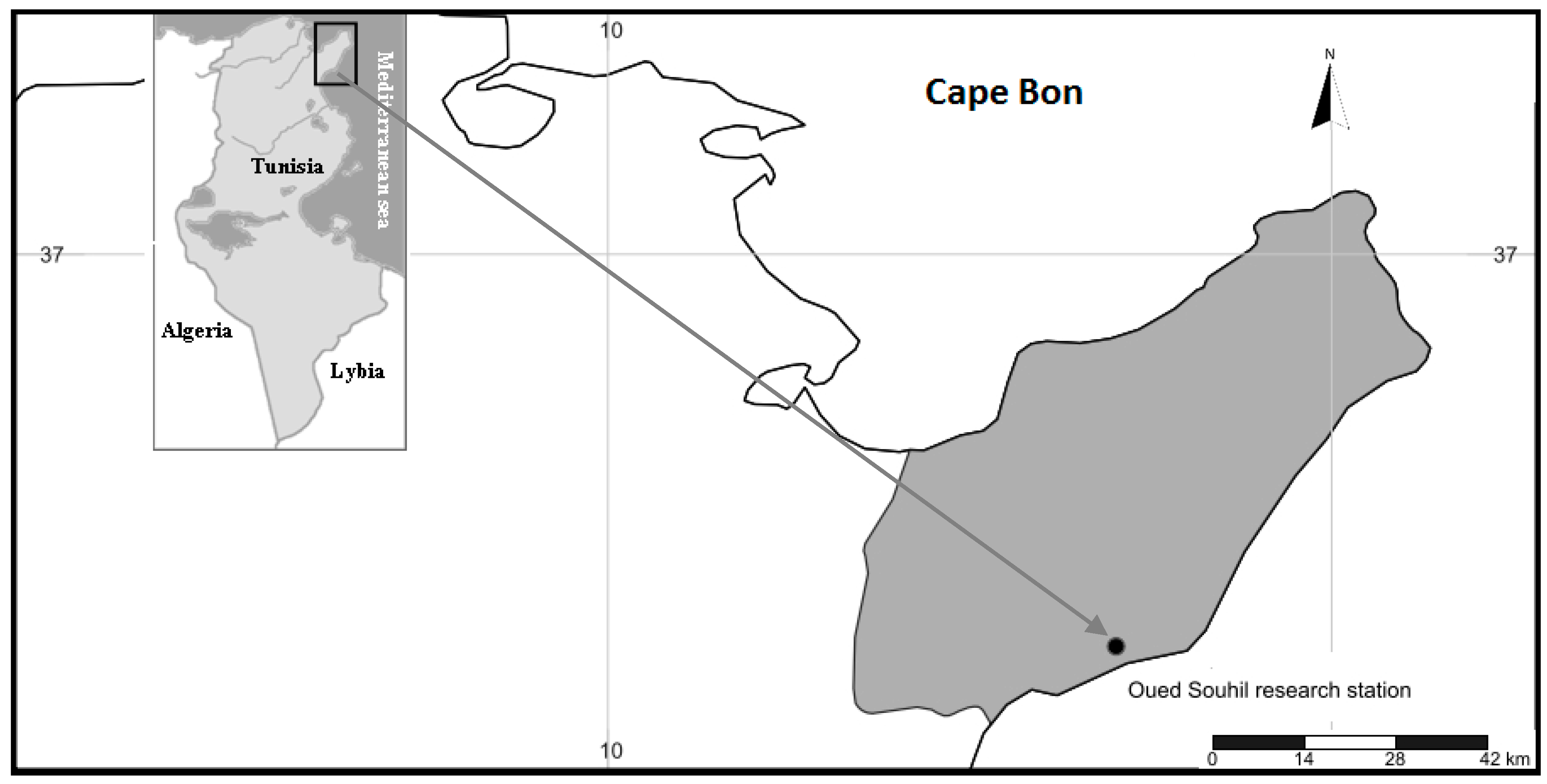
2.1. Study Area

The field study was conducted at the Oued Souhil research station belonging to the National Institute of Water, Forest and Rural Engineering (INRGREF) and located in Nabeul (36°27′47.8″ N, 10°42′13.4″ E) (Cap Bon Peninsula, Northeast Tunisia) (Figure 1). Nabeul is characterized by Mediterranean semi-arid climate with an average annual precipitation and potential evapotranspiration of 450 mm and 1370 mm, respectively (calculated for the period 1982–2006). Rainfall is characterized by intra-annual and inter-annual variability. The driest month is July and the wettest is January. The average temperature in the study area is 26 °C during summer and 15 °C during winter. Water resources are provided principally from groundwater, transferred surface water from the north of the country. and reused treated waste water. The coastal aquifer system is formed by a complex multi-reservoir system formed by semi-confined multilayers filled with sand, sandstone, limestone, and sandy clay lithologies and interconnected to each other by leaky-confining aquitards [31]. These aquifers are almost threatened by over pumping for the water supply of agricultural, touristic, and industrial sectors needs to be lead to seawater intrusion. The electrical conductivity (EC) ranges from 0.73 to 10.12 dSm⁻¹ [32]. Surface drip irrigation, combined with the use of fertilizers and pesticides, is commonly practiced when cultivating potatoes in the region.

2.2. Soil Water Content and Salinity Monitoring

The experimental work was performed during a full growing season of a drip irrigated potato plot (from sowing date (11/03/2015) to harvest (07/07/2015)). The plot was left in fallow the cropping season before. The soil has a coarser texture and the water table is located at about 9 m below the soil surface. Thus the groundwater is deep enough to prevent water logging and salinization problems linked to capillary rise. During the experiment, irrigation water electrical conductivity (ECw), pH and Sodium Adsorption Ratio (SAR) were equal to 4.45 dSm⁻¹, 7.54 and 8.9 (mmol·l⁻¹)^0.5, respectively. Before installing the drip irrigation system, the field was ploughed to a depth of 0.5 m and all vegetation was removed. The experimental protocol was installed in a field of about 500 m², two regimes of irrigation were adopted: 100% (full irrigation) and 70% (deficit irrigation) of crop water requirement (ETc). The same agricultural practices were conducted for both irrigation treatments. From a total of 12 experimental micro plots (4 m × 3 m), a central plot with 100% ETc was selected for the soil water content and salinity real time monitoring. Each micro plot of 12 m² had 4 drip lines and the distances between drip lines and emitters were 0.8 m and 0.3 m respectively. The emitters flow rate was 3 l h⁻¹ and assumed constant throughout the system during each irrigation event. This was confirmed by multiple flow measurements during each irrigation event and by a water-meter. Potato yield was performed for both treatments.

Before irrigation and seeding the potatoes, the soil was sampled at 5 depth intervals (0–0.2, 0.2–0.4, 0.4–0.6, 0.6–0.8, 0.8–1.0 m) to measure the initial soil properties (soil particle size, soil water content, electrical conductivity of soil saturated extracts ECe, bulk density, and pH) according to USDA (1954) methods [33]. Soil samples were first dried in an oven at 105 °C for 24 h, and passed through a 2 mm mesh sieve. Soil particle size distribution was measured using the sedimentation method (pipette and hydrometer), soil pH was measured in the saturated soil paste extract, and soil bulk density was determined using undisturbed soil samples (cylinder method) for the soil layer 0–1.0 m. According to USDA (1954) soil textural classification, the soil is mainly sandy loam. The clay varied from 4% at surface soil and increased to 19% at deeper soil layers (

Table 1. Soil physical properties.

Particle Size Distribution (%)
Soil Depth (m)	Clay (d < 2 μm)	Silt (2≤ d < 50 μm)	Sand (50 ≤ μm d < 2 mm)	Bulk Density (g·cm−3)
0–0.2	4	25	70	1.41
0.2–0.4	15	11	73	1.52
0.4–0.6	16	12	71	1.69
0.6–0.8	19	11	70	1.73
0.8–1.0	17	11	70	1.81

).

Real time monitoring was implemented using Decagon 5TE probes (Decagon Devices Inc., Pullman, WA, USA), measuring hourly soil water content θ, temperature T, and pore electrical conductivity ECsw. Decagon-5TE is a capacitance probe (frequency domain reflectometry method (FDR)) and has three 5.2 cm long prongs with 1 cm spacing between adjacent prongs. Using an oscillator running at 70 MHz, 5TE probe measures soil permittivity Ka, bulk electrical conductivity EC_b, and soil temperature T. Four 5TE sensors were installed at four soil depths (0.05 m, 0.25 m, 0.45 m and 0.90 m). This investigation depth was chosen because potatoes have a shallow root system and water uptake is limited to soil depth 0.40 to 0.60 m [34]. 5TE probes were connected to the Decagon Em50 data logger for real time reading and saving the 5TE measures. The DataTrac3 software version 3.15 (Decagon Devices Inc., Pullman, WA, USA) was used to download the collected data from Em50 and to estimate θ and ECsw using Topp et al. [35] and Hilhorst [36] models, respectively.

2.3. Crop Requirement Calculation

Spunta-potato, the species used in this experiment, is consumed by many people all over the world. Its tubers are very regular, with large caliber and yellow skin. Spunta-potato duration cropping cycle is between 120–150 days with 500 mm/ha to 700 mm/ha consumption of water requirement in a semi-arid area [34]. The crop evapotranspiration (ETc) was determined by multiplying the reference crop evapotranspiration ET₀ with the crop coefficient Kc. The potato growth stages were determined based on field observations of leaf development, and the stem’s height. The crop growth cycle was roughly divided into four stages: initial from 11 to 31 March 2015, development from 1 April to 5 May 2015, midterm from 5 May to 19 June 2015 and late season from 19 June to 10 July 2015. According to the Food and Agriculture Organization (FAO) [37], initial Kc (Kcini) midterm Kc (Kcmid), and final Kc (Kcend) were equal to 0.5, 1.15, and 0.754, respectively. Cropwat8.0 was used to estimate ETc. The software requires climatic data, soil texture, soil water content at wilting point and field capacity, crop specific coefficient (Kc), and crop cycle growth to estimate the crop water requirement. During the potato season which lasted 101 days (from 11/3/2015 to 7/7/2015), the amount of full irrigation was about 336 mm allocated in 16 applications while rainfall was only about 20 mm. During the calculation period (from March 2015 to December 2016) rainfall was about 638 mm.

Besides we followed up an irrigation schedule practiced by a farmer applied to a drip potato plot located close to our research experimental station. A water meter was installed to record the amount and frequency of the applied irrigation water. The farmer irrigated with similar water quality and cultivated the same potato species. The purpose was to use the irrigation schedule for management scenarios run with HYDRUS-1D. The total amount of applied irrigation was 825 mm corresponding to 237% ETc. Daily irrigation doses varied from 7.5 mm to 37.5 mm and were applied almost until harvest. Unfortunately the yield obtained by this farmer was not available.

2.4. Modelling Approach

The modelling study was carried out using HYDRUS-1D code [27]. The model numerically simulates one-dimensional (1D) water flow, solute, and heat transport in variably-saturated porous media.

2.4.1. Water Flow, Solute Transport, and Root Water Uptake

HYDRUS-1D solves numerically the Richards’s equation (1), using Galerkin finite-element schemes:

$$\frac{\partial \theta }{\partial t}=\frac{\partial }{\partial z}\left[K\left(\frac{\partial h}{\partial z}+1\right)\right]-S,$$

(1)

where h is the water pressure head [L], θ is the volumetric water content [L³·L⁻³], t is time [T], z is the spatial coordinate [L] (positive upward), S is the sink term [L³·L⁻³·T⁻¹] (takes into account root water uptake). K is the unsaturated hydraulic conductivity function [L·T⁻¹] [27].

The HYDRUS-1D program implements Van Genuchten–Mualem soil-hydraulic functions for representing soil hydraulic properties [27]. The soil retention function, as initially proposed by Van Genucthen (1980) [38], is given by Equations (2) and (4) while the hydraulic conductivity function as presented by Mualem (1976) [39] is described by Equation (3):

$$\theta \left(h\right)=\{\begin{array}{ll}{\theta }_r+\frac{{\theta }_s-{\theta }_r}{{\left(1+{\left|\alpha h\right|}^n\right)}^m}& h<0\\ {\theta }_s& h\ge 0\end{array},$$

(2)

$$K(h)=K_s{S}_e^{0.5}{\left[1-{\left(1-S_e^{1/m}\right)}^m\right]}^2,$$

(3)

$$Se=\frac{\theta -{\theta }_r}{{\theta }_s-{\theta }_r},$$

(4)

where θ_s is the saturated water content [L³L⁻³, α [L⁻¹], n, m (= 1 − 1/n, n > 1) are empirical parameters, θ_r is residual water content [L³L⁻³], Se is effective water content and Ks is saturated hydraulic conductivity [L·T⁻¹].

Hydrus-1D also solves the advection–dispersion equations (CDE) for heat transfer and solute transport. Solute transport equations consider advective–dispersive transport, and diffusion [28].

$$\frac{\partial \theta C}{\partial t}=\frac{\partial }{\partial z}\left(\theta D\frac{\partial C}{\partial z}\right)-\frac{\partial v\theta C}{\partial z},$$

(5)

where C is the solute concentration of the liquid phase [M·L⁻³], D is the dispersion coefficient [L²·T⁻¹], and v is the average pore water velocity [L·T⁻¹]. When ignoring molecular diffusion, the dispersion coefficient is defined as:

D = λ v,

(6)

where λ is dispersivity (L). The dispersivity is viewed as a material constant independent of the flow rate. Dispersivity is the only solute transport parameter needed for solving the CDE equation for non-reactive solute transport modelling.

2.4.2. Root Water Uptake, Osmotic Stress Effect, and Yield Calculation

Root water uptake is a sink term in the Richards’s equation (1) defined as the volume of water removed from a unit volume of soil per unit time by the plant. The Feddes model [40] was considered for the present study as the water stress response function, and parameters for potato crop, available in HYDRUS-1D, were applied (P0 = −10 cm, Popt = −25 cm, P2H = −300 cm, P2L = −500 cm, P3 = −16000 cm, r2H = 0.50 cm/day, and r2L = 0.1 cm/day). P0 corresponds to the pressure head below which roots start to extract water from the soil. P2H is the value of the limiting pressure head below which roots can no longer extract water at the maximum rate (assuming a potential transpiration rate of r2H). P2L, is as P2H but for a potential transpiration rate of r2L. Root water uptake is set to zero for pressure heads less than the wilting point P3. Water uptake is considered optimal between pressure heads Popt and P2 (P2H and P2L), whereas for pressure heads between P2 and P3 (or P0 and Popt) water uptake decreases (or increases) linearly with pressure head. Root depth was set to 60 cm as defined by the FAO [34].

The osmotic effects of pore water salinity on root water uptake were considered by applying a threshold–slope function [41] with a slope (s) of 6% and a threshold value (ECt) of 3.40 dSm⁻¹ suggested in the HYDRUS1D crop parameters database. Further on, water and salinity effects on root water uptake were considered multiplicative. Maas and Hoffman [42] found that when the threshold salinity value was reached, plant growth and yield decreased linearly with increasing salinity. Ben-Gal et al. [43] confirmed that this linear relationship is valid for salinity stress as well as water deficiency. As most models do not integrate complex plant growth, simulated root water uptake (actual transpiration) is considered to be a good indication of the crop yield. Oster et al. [44] defined the relative yield Yr (%) as the ratio between the value of the actual root extraction (provided by the software as output) and the value of the potential or maximum root extraction corresponding to potential transpiration. The observed average yield, which was set to 25 T/ha, was derived from former studies performed in Tunisia [45]. For the present study, the measured yield for the treatment 70% ETc and 100% ETc was equal to 13.14 T/ha and 17.89 T/ha, respectively.

2.4.3. Boundary and Initial Conditions

HYDRUS-1D was applied on a 1 m soil profile composed of four material layers. The model offers several possibilities for the top and bottom boundary conditions regarding flow transport. Atmospheric boundary conditions (BC) with surface runoff were considered at the top of the profile. The potential water flux across the upper boundary is controlled by external conditions. However, the soil surface BC may change from a prescribed flux to a prescribed head type condition and vice-versa, depending on the prevailing (transient) soil moisture conditions. Daily potential values of evaporation, irrigation, and precipitation were added as variable boundary conditions. In the present work, the Penman–Monteith equation was used to estimate the reference crop evapotranspiration rate, ET₀ (mm) using daily radiation, air temperature, air humidity, and wind speed data recorded in the Nabeul climatic station (36°28′43.16″ N, 10°42′24.84″ E) [37,46]. Crop evapotranspiration ETc (mm) was then calculated using the product of ET₀ and Kcini, Kcmid, and Kcend.

The HYDRUS-1D atmospheric boundary condition requires inputting separately evaporation and transpiration. To split ET_c into potential evaporation (Ep) and potential transpiration Tp, we applied equation (7) proposed by Ritchie [47]:

$$\begin{array}{l}Tp=ETc\times SCF\\ Ep=ETc\times (1-SCF)\\ SCF=1-Exp\left(-0.46\times LAI\right)\end{array},$$

(7)

where SCF is the Surface Cover Fraction estimated from the Leaf Area Index (LAI). Evapotranspiration, evaporation, and transpiration are expressed in mm. LAI values were derived from the literature [48] and introduced according to the stages of the potato cycle. At the initial stage, LAI was equal to 1.2 m²·m⁻² and then reached 3.5 m²·m⁻² (LAImax), at the end-season it decreased to 1.3 m²·m⁻² [48].

Solute upper boundary condition was assigned as a concentration flux. Measured salinity of the irrigation water was thus applied as the upper solute BC. Free drainage and zero concentration gradient were considered as respectively flow and solute bottom boundary conditions. Initial conditions of water content and salinities were derived from field observations.

2.4.4. Model Calibration and Validation

Soil hydraulic parameters were first estimated using the Rosetta pedotransfer function integrated in HYDRUS-1D [49], based on particle size distribution and bulk density measured values for the five soil layers. Dispersivity (λ) was first set equal to one-tenth of the profile depth. Inverse modelling proposed in HYDRUS-1D, using an optimization approach based on the Marquardt–Levenberg method [27] was then used to calibrate soil (α, n, and Ks) and transport (λ) parameters. Soil hydraulic and transport parameters were calibrated and validated using field data collected from 6 May to 23 June 2015 (38 days for calibration and 12 days for validation). Objective function observation inputs for inverse modeling corresponded to 12 events for the four soil layers.

Model performance, for soil water content and salinity, was evaluated using both the Root Mean Square Error (RMSE) and determination coefficient (R2) indicators: RMSE values indicate the differences between observed and predicted values by the model. The closer the RMSE values are to zero, the better the model predicts the parameter.

2.4.5. Irrigation Management Scenarios

The treatments consisted of water replacement of the accumulated crop evapotranspiration (ETc) at levels of 70% (T1) and 237% (T3) corresponding to the irrigation schedule practiced by the followed farmer. Besides studying the effects of water and solute stress on root water uptake (T1S, T2S and T3S), we considered three scenarios T1R, T2R, and T3R where we extended the simulation period to two subsequent rainfall seasons and where the field was left in fallow for the following crop season (

Table 2. Simulation scenarios.

Main Scenarios	Detailed Scenarios
Root water uptake and yield predictions	T1	Irrigation with 70% crop water requirement (ETc)
	T2	Irrigation with 100% crop water requirement (ETc)
	T3	Irrigation with 237% crop water requirement (ETc)
	T1S	Irrigation with 70% crop water requirement (ETc) and Salinity stress effect
	T2S	Irrigation with 100% crop water requirement (ETc) and Salinity stress effect
	T3S	Irrigation with 237% crop water requirement (ETc) and Salinity stress effect
Leaching scenarios (661days)	T1R	Irrigation with 70% ETc and atmospheric Boundary Conditions extended to December 2016
	T2R	Irrigation with 100% ETc and atmospheric Boundary Conditions extended to December 2016
	T3R	Irrigation with 237% ETc and atmospheric Boundary Conditions extended to December 2016

). Soil column was also extended from 1 to 9 m (groundwater depth fluctuated between 11 to 9 m) in HYDRUS-1D for the latter simulations to estimate the solute return flows.

3. Results and Discussion

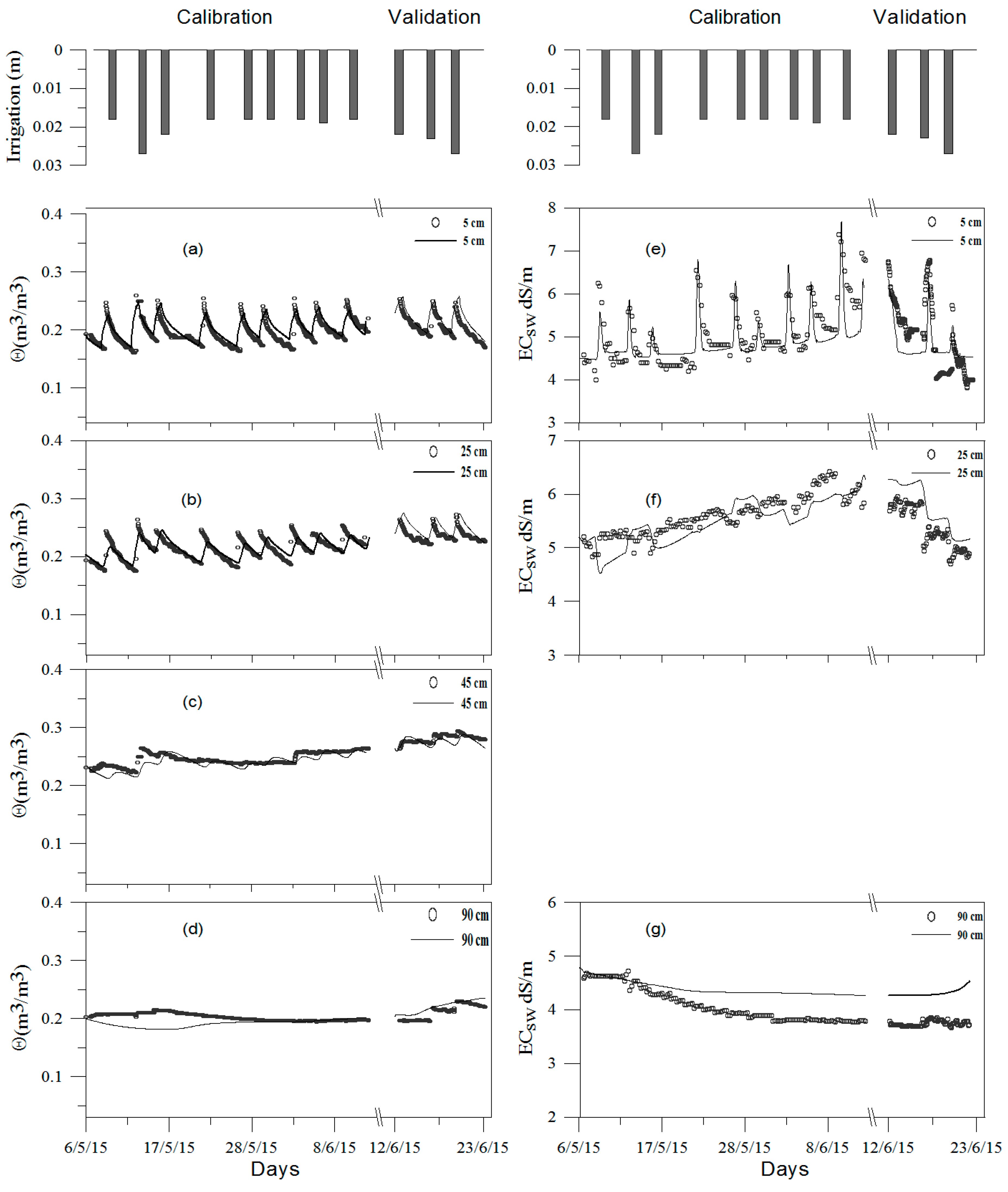
3.1. Water Content and Salinity Dynamics Evolution under Irrigation

Before irrigation started, the soil salinity ECe of the first field campaign (T₀) (19/03/2015) was equal to 1.4 dSm⁻¹ in the root zone (0–0.6 m). In the soil layer 0–1.5 m, we observed a leached soil salinity profile with ECe increasing from the surface to 1.50 m. This result and the low observed soil salinity could be explained by the natural leaching under rainfall. In fact, the plot was left in fallow for the two previous crop seasons.

Figure 2 shows the temporal evolution of the observed water contents and salt dynamics under irrigation for the four observed layers (0–0.10 m, 0.10–0.30 m, 0.30–0.50 m (only water content), and 0.50–1.0 m) (T2S). Observed values of salinity for the layer 0.30–0.50 m were not considered in the discussion because the probe was giving inappropriate measures of bulk electrical conductivity (EC_b). Water content increased at each irrigation event following the peaks reaching 0.26 m³·m⁻³ and decreased then to 0.16 m³·m⁻³ under root water uptake and evaporation. These fluctuations were obviously more visible and presented more intense peaks in the surface soil layers of 0–0.30 m, more influenced by soil plant atmosphere exchanges than the deeper layers of 0.30–1.0 m which presented a relatively constant water content. Li [29] explained that these layers served as a soil moisture buffer layer.

Similarly, measured ECsw was mainly impacted by irrigation events (Figure 2). Salinity troughs were mostly observed under irrigation, as water content θ and ECsw presented an opposed trend. Indeed, irrigation water volumes increased soil moisture, and diluted soil solution inducing ECsw decrease. As for the water content, salinity fluctuations were mainly observed at the surface soil layer 0–0.05 m. ECsw reached 7.35 dSm⁻¹ at the maximum crop transpiration stage and the minimum of ECsw (3.6 dSm⁻¹) was observed just after the last recorded irrigation (Figure 2). Observed salinities at the end of the crop season were still higher than those measured before irrigation started. Slama [20] reported a high salinity (17 dSm⁻¹) at the surface of a sandy soil measured two months after the end of a drip irrigated tomato season and which dropped to 4 dSm⁻¹ after the rainfall season. The process of rainfall leaching of the accumulated salts will be discussed while presenting results of the management scenario treatments.

3.2. Model Calibration and Validation

The model generally succeeded in reproducing the 5TE measurements of soil water contents and salinity ECsw during the considered calibration and validation periods (Figure 2). Indeed goodness-of-fit indicators RMSE, and R² values were small and high respectively (

Table 3. Model performance indicators.

		Calibration		Validation
Water flow	Soil depth (m)	R2	RMSE (m3·m−3)	R2	RMSE (m3·m−3)
	0.05	0.91	0.009	0.93	0.010
	0.25	0.93	0.005	0.85	0.007
	0.45	0.83	0.005	0.69	0.010
	0.90	0.85	0.003	0.75	0.005
Solute transport	Soil depth (m)	R2	RMSE (dSm−1)	R2	RMSE (dSm−1)
	0.05	0.800	0.280	0.650	0.600
	0.25	0.700	0.190	0.810	0.160
	0.90	0.980	0.040	0.850	0.070

). Table 3 presents results of these indicators for each layer apart from water content and salinity simulations. Calibration periods resulted in mean RMSE = 0.005 m³·m⁻³ (from 0.003 to 0.009 m³·m⁻³) and mean R² = 0.88 (from 0.83 to 0.93) for soil water content and mean RMSE = 0.17 dSm⁻¹ (from 0.04 to 0.28 dSm⁻¹) and R² = 0.83 (from 0.70 to 0.98) for ECsw. The validation period resulted in mean RMSE = 0.008 m³m⁻³ (from 0.005 to 0.01 m³·m⁻³) and mean R² = 0.81 (from 0.69 to 0.93) for soil water, and mean RMSE = 0.28 dSm⁻¹ (from 0.07 to 0.6 dSm⁻¹) and mean R² = 0.77 (from 0.65 to 0.85) for ECsw (Table 3).

Former studies applying different versions of the HYDRUS model for simulating water content and non-reactive solute transport reported a similar range of goodness-of-fit indicators for water content [25,28,29,30] and for salinity [23,50]. Note that calibration goodness-of-fit indicators were slightly better than those obtained for validation (Table 3) a common occurrence according to Phogat et al. [50]. The main cause is probably linked to the fact that for the calibration period, irrigation frequency was higher, during the mid-crop season, than it was for the validation period occurring at the crop season end. Thus the model performed better for infiltration processes than for evaporation ones. Wegehenkel et al. [51] used HYDRUS-1D for computing evaporation and found that the model performance was different for the dry season compared to the wet season. They also noted that model discrepancies can be explained by the choice of the root water uptake model and the root depth and distribution. Ramos et al. [28] focused on the influence of the crop growth stage on transpiration and thus on the error between simulated and observed values of the water content computed by HYDRUS-2D. Soil heterogeneity and preferential flow paths are also reported as causes of differences between simulated and observed values. Comparing the goodness-of-fit indicators of HYDRUS-1D for water flow to those obtained for salinity, we noticed that the model was more accurate in reproducing water contents. The model overestimated (e.g., soil layer 50–100 cm) or underestimated salinity contents. Phogat et al. [50] experienced similar difficulties when modelling salinity using HYDRUS-2D and noted that it was more difficult than simulating water flow especially for low values of water contents. This could be explained by diverse geochemical processes occurring when irrigation water infiltrates the vadose zone such as dissolution/precipitation, adsorption/desorption [23], and rock water interaction [20].

The calibrated parameters of water flow (α, n, and Ks) and solute transport (λ) are shown in

Table 4. Calibrated soil hydrodynamic and solute transport parameter treatments.

Depth (m)	Θr (m3·m−3)	θs (m3·m−3)	α (m−1)	n (-)	Ks (m·day−1)	λ (m)
0–0.2	0.036	0.3938	3.32	1.69	2	0.005
0.2–0.4	0.0555	0.3947	4	1.60	1	0.006
0.4–0.6	0.0515	0.3571	3.14	1.50	0.28	0.004
0.6–0.8	0.051	0.3416	4	1.23	0.125	0.004
0.8–1.0	0.0507	0.3388	1	1.40	0.68	0.004

. They were compliant with those predicted by the neural network Rosetta model implemented in HYDRUS1-D. Selim et al. [5] also performed different drip irrigation treatment experiments in the same experimental site of Oued Souhil and found the same range of Ks, α, and n. Note that Ks decreased with depth because of sub-soil compaction at that depth. (60 cm) due to soil plowing also reported by González et al. [30]. Calibrated dispersivities (λ) were also similar to those cited in the literature [24,30].

Despite some discrepancies between measured and simulated values, the model was judged to be reliable to continue calculations for management scenarios of applied irrigation amounts.

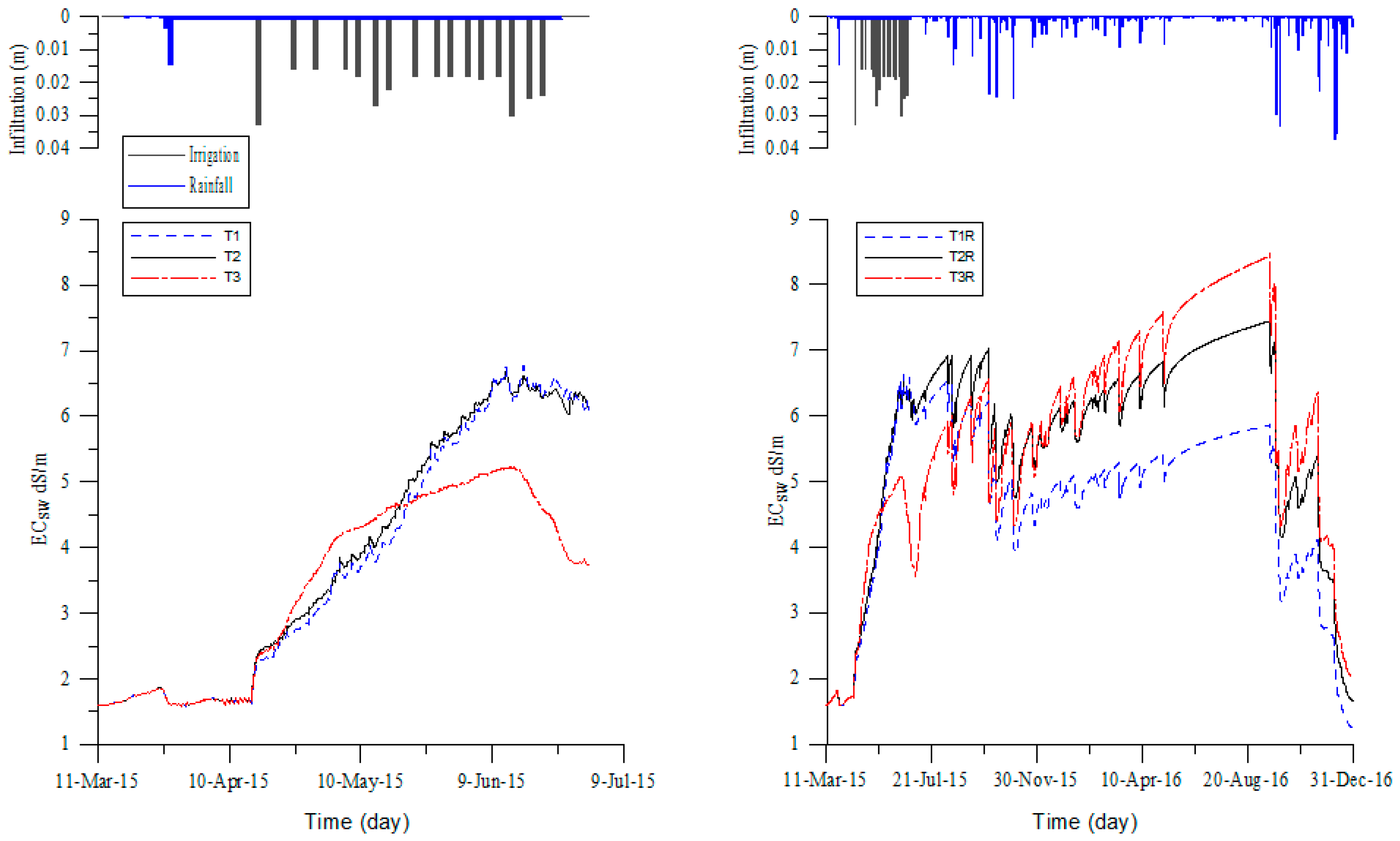
3.3. Irrigation Management Scenarios

Table 5. Calculated water balance for different treatments for the crop and rainfall season.

Scenario	Net Rainfall (mm)	Net Irrigation (mm)	Δ Soil Storage (mm)	Percolation (mm)	Actual Evaporation (mm)	Actual Transpiration (mm)	Input (mm)	Output (mm)	Water Balance Error (%)	Water Balance Error computed by HYDRUS-1D (%)
	R	I	ΔS	P	E	Tac	R + I	E + Tac + P+ ΔS
T1	20	235	−170	96	120	203	255	249	2.33	0.93
T2	20	336	−129	96	130	255	356	353	0.83	0.36
T3	20	825	327	96	138	263	845	824	2.48	1.91
	R	I	ΔS	P	E	Tac	R + I	E + Tac + P + S
T1S	20	235	−143	96	129	173	255	255	0.15	0.045
T2S	20	336	−105	96	138	225	356	355	0.33	0.064
T3S	20	825.07	327.20	96.43	137.50	262.92	845.07	824.05	2.49	1.91
	R	I	ΔS	P	E	Tac	R + I	E + Tac + P + S
T1R	638	235	−180	260	587	203	873	869	0.40	0.09
T2R	638	336	−165	260	619	255	974	970	0.40	0.054
T3R	638	825	−13	520	694	263	1463	1464	−0.08	0.027

shows the water balance components calculated for the different simulated treatments. Water balance error was calculated at the boundaries (cumulative fluxes) as follows:

$$\mathsf{\epsilon }=\frac{\left(R+I\right)-\left(E+Tac+\mathrm{P}+\Delta S\right)}{R+I}\times 100,$$

(8)

where R is net rainfall (mm), I is net irrigation (mm), ΔS is soil storage variation (mm), E is actual evaporation (mm), and Tac is actual transpiration (mm).

Besides, the relative error of water balance, computed by HYDRUS1-D [27] and indicating the accuracy of the numerical solution, is given in Table 5. Both water balance errors were acceptable and similar to values reported in the literature [30].

3.3.1. Root Water Uptake and Yield Estimations

Root water uptake reached 64.19%, 80.2%, and 85.54 % of its potential value for T1, T2, and T3 respectively. Results for T1, T2, and T3 treatments also showed that during the crop season, evaporation and transpiration (ie root water uptake) increased with the increase of the irrigation water amount. Note that For T3 corresponding to 237% of ETc, root water uptake increased by only 12 mm (4.7 %) compared to T2 (100% ETc). Besides, for T3 even with important quantities of irrigation we only reached 85.5% of potential root water uptake (crop yield). This is mainly explained by inadequate irrigation scheduling and doses impacting root zone pressure heads (ranging between −685 and −1.8 cm) and causing water logging and/or water stress.

However for T1 (70% ET_C) the root uptake amount decreased by 52 mm (20.4%) compared to T2 (100% ET_C).

When both water and solute stress are considered (treatments T1S, T2S, T3S) root water uptake decreased compared to the same treatments with only water stress (T2 and T1). Reduction in root water uptake (compared to T2) reached 32.3% and 11.6% for T1S and T2S respectively. However root water uptake for T3S remained the same as for T3. It is obvious that important amounts of irrigation applied in treatment T3 succeeded in leaching soil out of the root zone. Figure 3 presents the salinity evolution in the root zone (0–0.60 m) under different treatments. We noticed that during the irrigation season, salinity was the lowest for T3 compared to T1 and T2, yet it increased and became the highest in the dry season (during summer) under evaporation.

Estimated and observed relative yields are given in

Table 6. Estimated versus observed yields for different treatments.

Scenario	Calculated (HYDRUS1-D) Relative Yield Yr (%)	Observed Relative Yield Yr (%)
T1	64.2	52.6
T2	80.29	71
T3	85.5
T1S	54.2	52.6
T2S	70	71
T3S	85.5	-

. Root water uptake reduction due to solute stress resulted in yield reduction of about 10% for T1S and T2S in comparison to treatments without solute stress T1 and T2 respectively. Note that observed relative yields matched best with treatments taking into account solute stress, T1S and T2S.

These findings were already reported in other case studies. Nagaz et al. [52] performed a field study in southern Tunisia to determine the effect of irrigation regimes with saline water (3.25 dSm⁻¹) on soil salinity, yield, and water use efficiency of potato (Spunta) grown during different seasons in a sandy soil. Irrigation treatments consisted in full (100% ETc) and deficit irrigation (water replacements of ETc at levels of 80%, 60%, and 40%). They noted that the deficit irrigation treatments resulted in higher salinity in the root zone than the full irrigation treatments. The observed higher salinity, associated with deficit irrigation, caused important reductions in tuber yield and its components. Aragues et al. [7] conducted an RDI experiment on a table grape vineyard drip-irrigated with moderately saline, to assess soil salinization and soil sodification under this regime. They found that the grapevine yield declined with the increase in soil salinity and concluded that implementation of drip irrigation combined with RDI in low-precipitation semi-arid areas must be cautiously assessed and monitored because of soil salinization and sodification.

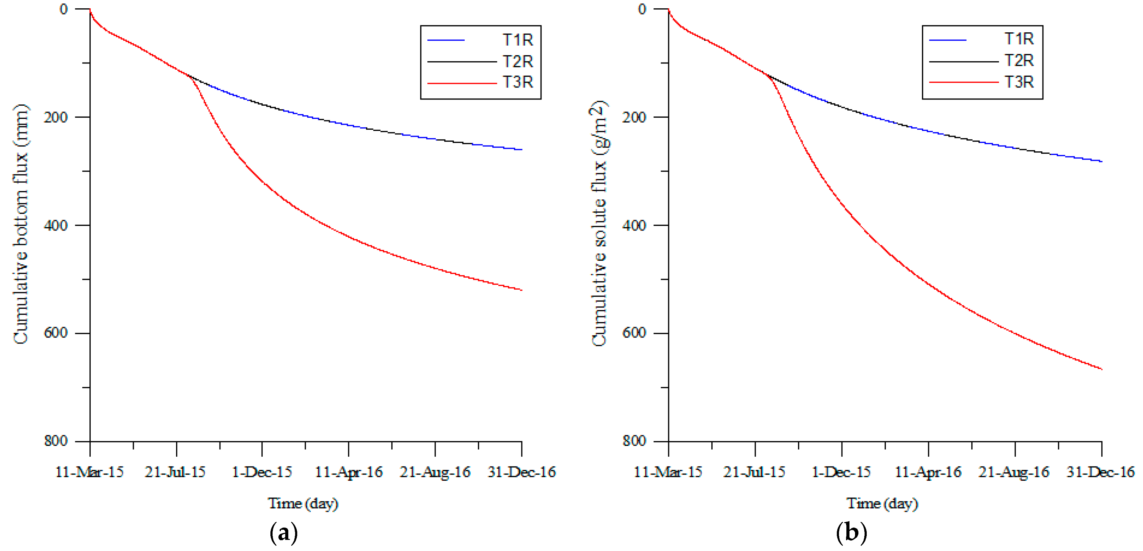
3.3.2. Impact on Solute and Water Return Flows

The HYDRUS-1D estimation for percolation was about 96 mm for the three treatments T1, T2, and T3, however variations in soil storage, for these scenarios, were different and increased with the irrigation amount increase. Percolation values were higher for treatments T1R, T2R, and T3R considering the two subsequent rainfall seasons. The percolation amount was the highest for T3R with 520 mm whereas it was equal, for T1R and T2R with a value of 260 mm (Figure 4). The influence of rainfall on percolation values of T3R was thus obviously higher; this is due to the important amount of irrigation which was not taken by plant roots and remained stored in the soil.

Consequently, this amount of irrigated water (T3R), concentrated with solutes (4.45 dSm^–1), resulted in the highest bottom solute flux, reaching groundwater with a value of 680 g/m² (6800 T/ha) (Figure 4). For T1R and T2R solute fluxes were estimated at 280 g/m². When examining the figure describing root zone salinity one can notice that for T3R, salinity was the lowest during the crop season as the irrigation amounts leached salinity out of the root zone but then solute mobilization was enhanced in summer under evaporation and capillary rise, ending up with the highest salinity among the treatments. Conversely, salinity under deficit irrigation (T1R) increased during crop season but then presented the lowest increase under evaporation and the highest decrease under rainfall.

Note that leaching processes were most active within important events of rainfall that took place in September (from 25 to 30th cumulative rainfall = 63 mm) and December 2016 (from 7 to 9th cumulative rainfall = 226 mm with 153 mm recorded on the 8th). Slama et al. [53] found that rainfall structure had a noticeable impact on the solute leaching processes. Also, in arid and semi-arid Tunisia, the impact of rainfall on soil desalinization was more important for coarse than fine soil texture irrigated with brackish water [54].

Several studies reported the impact of irrigation return fluxes on groundwater quality and salinization processes in arid and semi-arid lands [18,20,55]. At a large scale, solute recycling can be estimated as a function of the solute mass extracted from pumping wells [19] but different irrigation regimes have different salt leaching effects [56]. As an example flood irrigation, is able to decrease soil salt content, but it also has an adverse effect on the environment because the huge amount of water leads to deep seepage which increases the salinization risk of the aquifer [23,24].

4. Conclusions

Observed data demonstrated that salinity increased in the root zone during the crop season under irrigation with brackish water. As a consequence observed yields were lower than the optimum ones recorded in the region for the potato crop for both full and deficit irrigation treatments.

Simulation results showed that HYDRUS-1D was an effective tool for evaluating water and solute transport under full irrigation as goodness-of-fit indicators were acceptable and conform to those found in the literature. Subsequently management scenarios corresponding to deficit and over irrigation regimes could then be performed. In addition, simulations were extended to two subsequent seasons of rainfall to investigate irrigation return fluxes under different irrigation regimes.

While it was obvious that deficit irrigation (T1R) resulted in a decrease in root water uptake and consequently in calculated and observed relative yields, the irrigation return fluxes and soil salinity after two subsequent rainfall seasons were the lowest among the considered scenarios (full irrigation and over irrigation). The irrigation amounts applied by the farmer (T3R) leached the salinity far from the root zone but then solutes were mobilized under evaporation in the dry season resulting in the highest salinities and solute return fluxes.

Considering these findings, it is important for researchers to perform long-term investigations in using deficit irrigation with saline irrigation water. The challenge is to consider not only yield decrease but also environmental impacts (salinization, sodification, and nitrate contamination) on soil and groundwater for different soil types. It is also of great interest to integrate the climate change consequences related to temperature rise and to the frequency of rainfall, extreme events having an important role in solute leaching.

References

1. Besbes, M.; Chahed, J.; Hamdane, A. Water Security, Food Security and the National Water Dependency. In National Water Security: Case Study of an Arid Country: Tunisia; Springer International Publishing: Cham, Switzerland, 2018; pp. 219–255. [Google Scholar]
2. Bouksila, F.; Persson, M.; Berndtsson, R.; Bahri, A.; Hamba, I.B. Estimating soil salinity over a shallow saline water table in semiarid Tunisia. Open Hydrol. J. 2010, 4, 91–101. [Google Scholar] [CrossRef]
3. Aragüés, R.; Pueyo, E.T.; Zribi, W.; Clavería, I.; Álvaro-Fuentes, J.; Faci, J. Soil Salinization as a threat to the sustainability of deficit irrigation under present and expected climate change scenarios. Irrig. Sci. 2015, 33, 67–79. [Google Scholar] [CrossRef]
4. Liao, L.; Zhang, L.; Bengtsson, L. Soil moisture variation and water consumption of spring wheat and their effects on crop yield under drip irrigation. Irrig. Drain. Syst. 2008, 22, 253–270. [Google Scholar] [CrossRef]
5. Selim, T.; Bouksila, F.; Berndtsson, R.; Persson, M. Soil Water and Salinity Distribution under Different Treatments of Drip Irrigation. Soil Sci. Soc. Am. J. 2013, 77, 1144–1156. [Google Scholar] [CrossRef]
6. Al Atiri, R. Les efforts de modernisation de l’agriculture irriguée en Tunisie. In Proceedings of the Projet Européen Inco-Wademed sur la Modernisation de L’agriculture Irriguée Dans les pays du Maghreb, Cahors, France, 6–7 Novembre 2006; pp. 19–22. [Google Scholar]
7. Aragüés, R.; Medina, E.T.; Clavería, I.; Martínez-Cob, A.; Faci, J. Regulated deficit irrigation, soil salinization and soil sodification in a table grape vineyard drip-irrigated with moderately saline waters. Agric. Water Manag. 2014, 134, 84–93. [Google Scholar] [CrossRef] [Green Version]
8. Mounzer, O.; Pedrero-Salcedo, F.; Nortes, P.A.; Bayona, J.-M.; Nicolas-Nicoas, E.; Alarcon, J.J. Transient soil salinity under the combined effect of reclaimed water and regulated deficit drip irrigation of Mandarin trees. Agric. Water Manag. 2013, 120, 23–29. [Google Scholar] [CrossRef]
9. Leite, K.N.; Martinez-Romero, A.; Tarjuelo, J.M.; Dominguez, A. Distribution of limited irrigation water based on optimized regulated deficit irrigation and typical metheorological year concepts. Agric. Water Manag. 2015, 148, 164–176. [Google Scholar] [CrossRef]
10. Allen, M.; Barros, V.; Broome, J.; Cramer, W.; Christ, R.; Church, J.; Clarke, L.; Dahe, Q.; Dasgupta, P.; Dubash, N.; et al. IPCC Fifth Assessment Synthesis Report—Climate Change 2014 Synthesis Report; Intergovernmental Panel on Climate Change (IPCC): Geneva, Switzerland, 2014; p. 116. [Google Scholar]
11. El Jaouhari, N.; Abouabdillah, A.; Bouabid, R.; Bourioug, M.; Aleya, L.; Chaoui, M. Assessment of sustainable deficit irrigation in a Moroccan apple orchard as a climate change adaptation strategy. Sci. Total Environ. 2018, 642, 574–581. [Google Scholar] [CrossRef] [PubMed]
12. Geerts, S.; Raes, D. Deficit irrigation as an on-farm strategy to maximize crop water productivity in dry areas. Agric. Water Manag. 2009, 96, 1275–1284. [Google Scholar] [CrossRef] [Green Version]
13. Fan, X.; Fei, C.; McCarl, B. Adaptation: An Agricultural Challenge. Climate 2017, 5, 56. [Google Scholar] [CrossRef]
14. Smedema, L.K.; Shiati, K. Irrigation and salinity: A perspective review of the salinity hazards of irrigation development in the arid zone. Irrig. Drain. Syst. 2002, 16, 161–174. [Google Scholar] [CrossRef]
15. Besbes, M.; Chahed, J.; Hamdane, A. The National Water Balance. In National Water Security: Case Study of an Arid Country: Tunisia; Springer International Publishing: Cham, Switzerland, 2018; pp. 93–123. [Google Scholar]
16. DGACTA. Examen et Evaluation de la Situation Actuelle de la Salinization des Sols et Préparation d’un Plan D’action de Lutte Contre ce Fléau Dans les Périmètres Irrigués en Tunisie. Phase 2: Ebauche du Plan D’action; DGACTA, Ministère de L’agriculture et des Ressources Hydrauliques: Tunis, Tunisia, 2007.
17. Marlet, S.; Bouksila, F.; Bahri, A. Water and Salt Balance at Irrigation Scheme Scale: A Comprehensive Approach for Salinity Assessment in a Saharan Oasis. Agric. Water Manag. 2009, 96, 1311–1322. [Google Scholar] [CrossRef]
18. Aragüés, R.; Tanji, K.K.; Quílez, D.; Alberto, F.; Faci, J.; Machín, J.; Arrué, J.L. Calibration and verification of an irrigation return flow hydrosalinity model. Irrig. Sci. 1985, 6, 85–94. [Google Scholar] [CrossRef] [Green Version]
19. Yakirevich, A.; Weisbrod, N.; Kuznetsov, M.; Rivera Villarreyes, C.A.; Benavent, I.; Chavez, A.M.; Ferrando, D. Modeling the impact of solute recycling on groundwater salinization under irrigated lands: A study of the Alto Piura aquifer, Peru. J. Hydrol. 2013, 482, 25–39. [Google Scholar] [CrossRef]
20. Slama, F. Field Experimentation and Modelling of Salts Transfer in Korba Coastal Plain: Impact of Seawater Intrusion and Irrigation Practices. Ph.D. Thesis, University of Neuchatel, Neuchâtel, Switzerland, 2010. [Google Scholar]
21. Causapé, J.; Quìlez, D.; Aragüès, R. Irrigation efficiency and quality of irrigation return flows in the Ebro river basin: An overview. Environ. Monit. Assess. 2006, 117, 451–461. [Google Scholar] [CrossRef] [PubMed]
22. Causapé, J.; Quılez, D.; Araqüés, R. Assessment of irrigation and environmental quality at the hydrological basin level II. Salt and nitrate loads in irrigation return flows. Agric. Water Manag. 2004, 70, 211–228. [Google Scholar]
23. Kanzari, S.; Hachicha, M.; Bouhlila, R.; Battle-Sales, J. Characterization and modeling of water movement and salts transfer in a semi-arid region of Tunisia (Bou Hajla, Kairouan): Salinization risk of soils and aquifers. Comput. Electron. Agric. 2012, 86, 34–42. [Google Scholar] [CrossRef]
24. Zeng, W.; Xu, C.; Wu, J.; Huang, J. Soil salt leaching under different irrigation regimes: HYDRUS-1D modelling and analysis. J. Arid Land 2014, 6, 44–58. [Google Scholar] [CrossRef]
25. Ramos, T.B.; Šimùnek, J.; González, M.G.; Martins, J.C.; Prazeres, A.; Pereira, L.S. Two-dimensional modeling of water and nitrogen fate from sweet sorghum irrigated with fresh and blended saline waters. Agric. Water Manag. 2012, 111, 87–104. [Google Scholar] [CrossRef]
26. Mallants, D.; Van Genuchten, M.; Simunek, J.J.; Jacques, D.; Seetharam, S. Leaching of Contaminants to Groundwater. In Dealing with Contaminated Sites. From Theory to Practical Applications; Swartjes, F.A., Ed.; Springer: Berlin, Germany, 2010; pp. 787–850. [Google Scholar]
27. Šimùnek, J.; Šejna, M.; Saito, H.; Sakai, M.; Van Genuchten, M.T. The Hydrus-1D Software Package for Simulating the Movement of Water, Heat, and Multiple Solutes in Variably Saturated Media, Version 4.0; Department of Environmental Sciences, University of California Riverside: Riverside, CA, USA, 2008; p. 315. [Google Scholar]
28. Ramos, T.B.; Šimùnek, J.; González, M.G.; Martins, J.C.; Prazeres, A.; Castanheira, N.L.; Pereira, L.S. Field evaluation of a multicomponent solute transport model in soils irrigated with saline waters. J. Hydrol. 2011, 407, 129–144. [Google Scholar] [CrossRef]
29. Li, H.; Yi, J.; Zhang, J.; Zhao, Y.; Si, B.; Hill, R.; Cui, L.; Liu, X. Modeling of Soil Water and Salt Dynamics and Its Effects on Root Water Uptake in Heihe Arid Wetland, Gansu, China. Water 2015, 7, 2382. [Google Scholar] [CrossRef]
30. González, M.G.; Ramos, T.B.; Carlesso, R.; Paredes, P.; Petry, M.T.; Martins, J.D.; Aires, N.b.P.; Pereira, L.S. Modelling soil water dynamics of full and deficit drip irrigated maize cultivated under a rain shelter. Biosyst. Eng. 2015, 132, 1–18. [Google Scholar] [CrossRef]
31. Kallali, H.; Anane, M.; Jellali, S.; Tarhouni, J. GIS-based multi-criteria analysis for potential wastewater aquifer recharge sites. Desalination 2007, 215, 111–119. [Google Scholar] [CrossRef]
32. Moussa, A.B.; Zouari, K.; Marc, V. Hydrochemical and isotope evidence of groundwater salinization processes on the coastal plain of Hammamet—Nabeul, north-eastern Tunisia. Phys. Chem. Earth Parts A/B/C 2011, 36, 167–178. [Google Scholar] [CrossRef]
33. Richards, L.A. Diagnosis and Improvement of Saline and Alkali Soils. Soil Sci. 1954, 78, 154. [Google Scholar] [CrossRef]
34. Doorenbos, J.; Kassam, A.H. Yield Response to Water-FAO Irrigation and Drainage Paper 33; FAO-Food and Agriculture Organization of the United Nations: Rome, Italy, 1979; p. 193. [Google Scholar]
35. Topp, G.C.; Davis, J.L.; Annan, A.P. Electromagnetic determination of soil water content: Measurements in coaxial transmission lines. Water Resour. Res. 1980, 16, 574–582. [Google Scholar] [CrossRef]
36. Hilhorst, M.A. A Pore Water Conductivity Sensor. Soil Sci. Soc. Am. J. 2000, 64, 1922–1925. [Google Scholar] [CrossRef]
37. Allen, R.G.; Pereira, L.S.; Raes, D.; Smith, M. Crop Evapotranspiration-Guidelines for Computing Crop Water Requirements-FAO Irrigation and Drainage Paper 56; FAO-Food and Agriculture Organization of the United Nations: Rome, Italy, 1998; p. 293. [Google Scholar]
38. Van Genuchten, M.T. A closed-form equation for predicting the hydraulic conductivity of unsaturated soils. Soil Sci. 1980, 44, 892–898. [Google Scholar] [CrossRef]
39. Mualem, Y. A new model for predicting the hydraulic conductivity of unsaturated porous media. Water Resour. Res. 1976, 12, 513–521. [Google Scholar] [CrossRef]
40. Feddes, R.A.; Kowalik, P.; Kolinska-Malinka, K.; Zaradny, H. Simulation of field water uptake by plants using a soil water dependent root extraction function. J. Hydrol. 1976, 31, 13–26. [Google Scholar] [CrossRef]
41. Maas, E.V. Crop salt tolerance. In Agricultural Salinity Assessment and Management ASCE Manuals and Report on Engineering Practice; Amercia Social Civil Eng: New York, NY, USA, 1990; Volume 71, pp. 262–304. [Google Scholar]
42. Maas, E.V.; Hoffman, G.J. Crop salt tolerance-current assessment. J. Irrig. Drain. Div. 1977, 103, 115–134. [Google Scholar]
43. Ben-Gal, A.; Karlberg, L.; Jansson, P.-E.; Shani, U. Temporal robustness of linear relationships between production and transpiration. Plant Soil 2003, 251, 211–218. [Google Scholar] [CrossRef]
44. Oster, J.D.; Letey, J.; Vaughan, P.; Wu, L.; Qadir, M. Comparison of transient state models that include salinity and matric stress effects on plant yield. Agric. Water Manag. 2012, 103, 167–175. [Google Scholar] [CrossRef]
45. Gharbi, F.; El Fahem, M. Conditions de compétitivité des semences de pomme de terre produites en Tunisie. Biotechnol. Agron. Soc. Environ. 2004, 8, 187–198. [Google Scholar]
46. Liu, Q.; Yang, Z.; Cui, B.; Tao, S. The temporal trends of reference evapotranspiration and its sensitivity to key meteorological variables in the Yellow River Basin, China. Hydrol. Process. 2010, 24, 2171–2181. [Google Scholar] [CrossRef]
47. Ritchie, J.T. Model for predicting evaporation from a row crop with incomplete cover. Water Resour. Res. 1972, 8, 1204–1213. [Google Scholar] [CrossRef]
48. Nasr, Z.; Zairi, A.; Bechir, B.N.; Oueslati, T. Détermination de la consommation en eau journaliére par bilan d’énergie des cultures annuelles (blé et pomme de terre). Evolution avec la biomasse et application au pilotage des irrigations. Ann. Inrgref. 2000, 114–125. [Google Scholar]
49. Schaap, M.G.; Leij, F.J.; van Genuchten, M.T. Rosetta: A computer program for estimating soil hydraulic parameters with hierarchical pedotransfer functions. J. Hydrol. 2001, 251, 163–176. [Google Scholar] [CrossRef]
50. Phogat, V.; Pitt, T.; Cox, J.W.; Šimùnek, J.; Skewes, M.A. Soil water and salinity dynamics under sprinkler irrigated almond exposed to a varied salinity stress at different growth stages. Agric. Water Manag. 2018, 201, 70–82. [Google Scholar] [CrossRef] [Green Version]
51. Wegehenkel, M.; Beyrich, F. Modelling hourly evapotranspiration and soil water content at the grass-covered boundary-layer field site Falkenberg, Germany. Hydrol. Sci. J. 2014, 59, 376–394. [Google Scholar] [CrossRef] [Green Version]
52. Nagaz, K.; Masmoudi, M.M.; Ben Mechlia, N. Soil Salinity and Yield of Drip-Irrigated Potato under Different Irrigation Regimes with Saline Water in Arid Conditions of Southern Tunisia. J. Agron. 2007, 6, 324. [Google Scholar]
53. Slama, F.; Gargouri-Ellouze, E.; Bouhlila, R. Impact of rainfall structure on modelling solute leaching in soil and groundwater. In Proceedings of the Congress on Groundwater and Global Change in the Western Mediterranean, Granada, Spain, 6–9 November 2017. [Google Scholar]
54. Bouksila, F.; Bahri, A.; Berndtsson, R.; Persson, M.; Rozema, J.; van der Zee, S. Assessment of Soil Salinization Risks under Irrigation with Brackish Water in Semiarid Tunisia. Environ. Exp. Bot. 2013, 92, 176–185. [Google Scholar] [CrossRef]
55. Milnes, E.; Renard, P. The problem of salt recycling and seawater intrusion in coastal irrigated plains: An example from the Kiti aquifer (Southern Cyprus). J. Hydrol. 2004, 288, 327–343. [Google Scholar] [CrossRef]
56. Nachabe, M.H.; Ahuja, L.R.; Butters, G. Bromide transport under sprinkler and flood irrigation for no-till soil condition. J. Hydrol. 1999, 214, 8–17. [Google Scholar] [CrossRef]
Figure 1. Map of the experimental site (Oued Souhil, Nabeul).
Water 11 00425 g001
Figure 2. Simulated (solid line) versus measured (dots) soil water content (θ) for soil depths (a) 5 cm, (b) 25 cm (c) 45 cm, and (d) 90 cm and pore electrical conductivity (ECsw) for soil depths (e) 5 cm, (f) 25 cm, and (g) 90 cm and applied irrigation amounts.
Water 11 00425 g002
Figure 3. Root zone salinity for different treatments under irrigation and rainfall.
Water 11 00425 g003
Figure 4. Cumulative (a) water and (b) solute bottom fluxes for different treatments calculated from 11 March 2015 to 31 December 2016.
Water 11 00425 g004