A Multi-Sourced Data Retrodiction of Remotely Sensed Terrestrial Water Storage Changes for West Africa


1
School of Earth Sciences and Engineering, Hohai University, Jiangning Campus, Nanjing 211100, China
2
Department of Geomatic Engineering, Kwame Nkrumah University of Science and Technology, Kumasi AK000-AK911, Ghana
*
Author to whom correspondence should be addressed.
Water 2019, 11(2), 401; https://doi.org/10.3390/w11020401
Submission received: 5 January 2019
/
Revised: 6 February 2019
/
Accepted: 21 February 2019
/
Published: 25 February 2019
(This article belongs to the Special Issue Satellite Remote Sensing and Analyses of Climate Variability)
Abstract
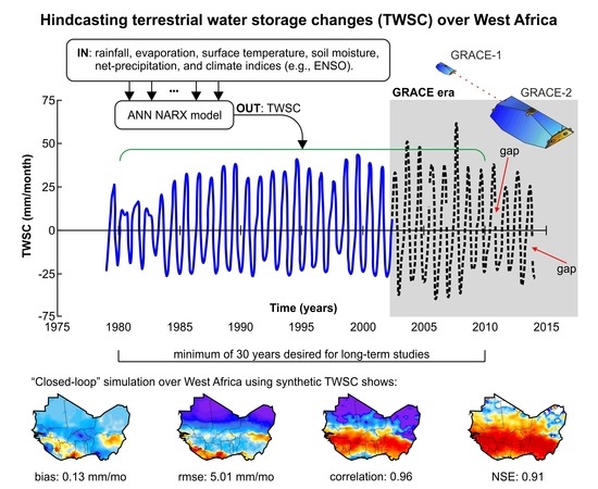
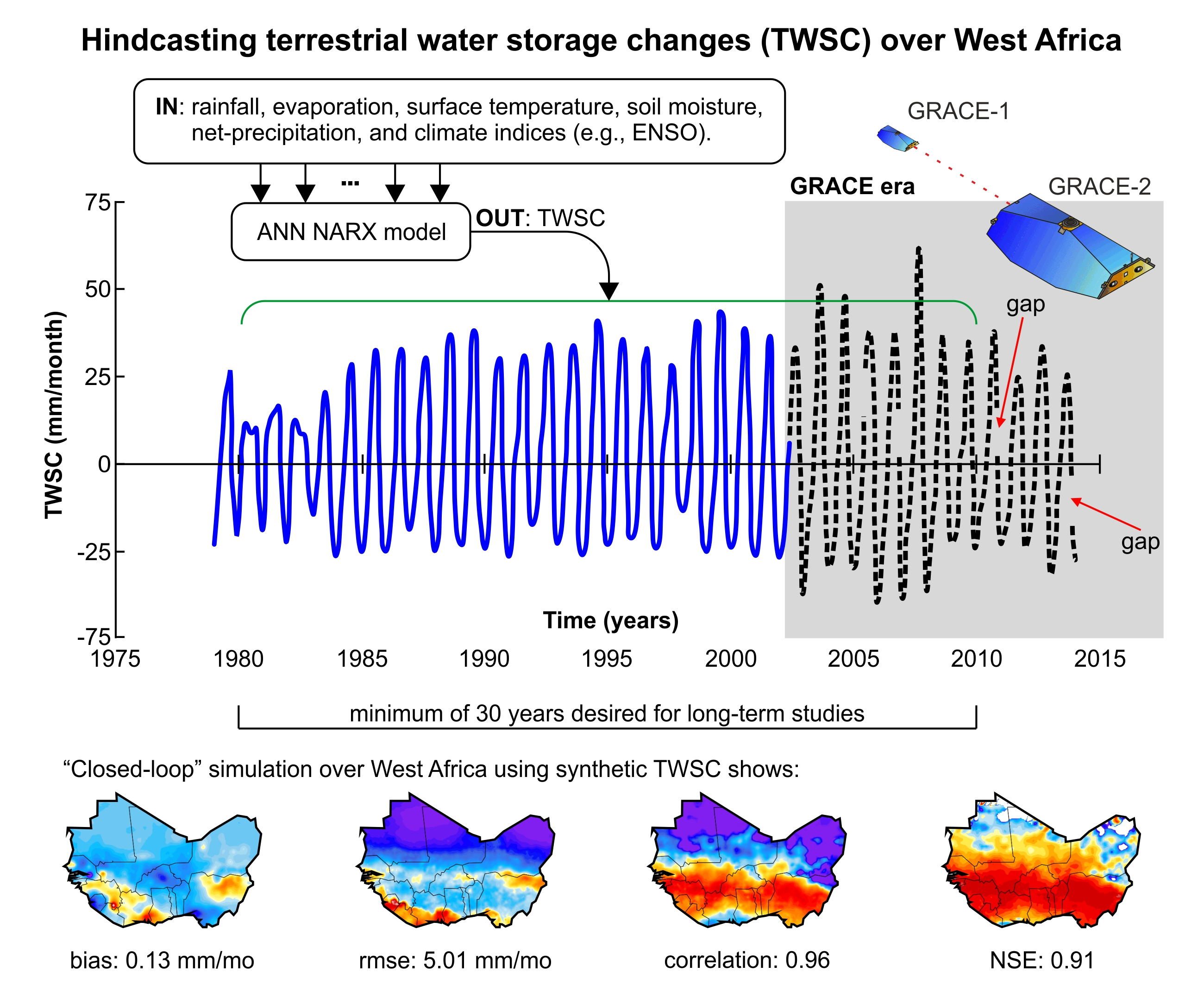
:Remotely sensed terrestrial water storage changes (TWSC) from the past Gravity Recovery and Climate Experiment (GRACE) mission cover a relatively short period (≈15 years). This short span presents challenges for long-term studies (e.g., drought assessment) in data-poor regions like West Africa (WA). Thus, we developed a Nonlinear Autoregressive model with eXogenous input (NARX) neural network to backcast GRACE-derived TWSC series to 1979 over WA. We trained the network to simulate TWSC based on its relationship with rainfall, evaporation, surface temperature, net-precipitation, soil moisture, and climate indices. The reconstructed TWSC series, upon validation, indicate high skill performance with a root-mean-square error (RMSE) of 11.83 mm/month and coefficient correlation of 0.89. The validation was performed considering only 15% of the available TWSC data not used to train the network. More so, we used the total water content changes (TWCC) synthesized from Noah driven global land data assimilation system in a simulation under the same condition as the GRACE data. The results based on this simulation show the feasibility of the NARX networks in hindcasting TWCC with RMSE of 8.06 mm/month and correlation coefficient of 0.88. The NARX network proved robust to adequately reconstruct GRACE-derived TWSC estimates back to 1979.
1. Introduction
A good understanding of regional hydrological conditions is vital to scientists, water resource managers, policy makers, among others, in helping to understand the state and flux of available freshwater. Such conditions are mostly evaluated with hydrological models, which enable the estimation and prediction of discharge and the various components of the terrestrial water storage. In West Africa (WA), the use of such models is nonetheless challenged by data scarcity [1]. Alternatively, global land surface models, such as, the Global Land Data Assimilation System (GLDAS) could be used to characterize hydrological conditions in the region [2]. However, these models perform poorly over the region due to the persistent issue of data deficiency [3]. The terrestrial water storage (TWS) inverted from the observations of the Gravity Recovery and Climate Experiment (GRACE) mission, therefore, is a very useful dataset which can be used to access changes in water availability to ensure a sustainable use [4]. However, the previous GRACE mission covered a relatively short period (April 2002 to July 2017), with 2 to 6 months latency, which makes it difficult to be used for long-term studies. Additionally, a data gap is envisaged between the past and the current (follow-on) GRACE missions. This, therefore, necessitates the need for an approach to forecast/backcast GRACE-derived TWS over the region.
As the variability of the water resources in WA is highly coupled to land-atmosphere-ocean interactions, both at the regional and global scales [5], it is reasonable to use hydro-climatic variables, such as rainfall, temperature, evaporation, and El Niño Southern Oscillation (ENSO) index, as retrieved from space-borne sensors, reanalysis datasets etc. to forecast/backcast TWS in the region. Using GRACE-derived TWS and in-situ river level records, Becker et al. [6] employed principal component analysis, which makes a linear and stationary assumption of time series to reconstruct GRACE-TWS from 1980 to 2008 over the Amazon basin. Similarly, de Linage et al. [7], developed a simple linear model between TWS over the Amazon and sea surface temperatures (SSTs) indices derived from Niño 4 and the Tropical North Atlantic Index (TNAI). Meanwhile, Forootan et al. [5], developed an autoregressive (ARX) model, which utilized independent component analysis (ICA) for dimension reduction to predict TWS over WA using rainfall data from the Tropical Rainfall Measuring Mission (TRMM), and SSTs of the three major oceanic basins (Pacific, Indian and Atlantic). However, this ICA/ARX method assumes a stationary state of TWS over the region and the prediction accuracy reduces after a forecast period of two years. Furthermore, Yin et al. [8] used the water balance method to extend the TWS series back to 1980 using multi-source datasets as inputs in the terrestrial water balance equation.
All the examples herein given require the use of mathematical models. It must be noted that, since the formulation of these models are based on empirical data, it essentially makes this a machine learning/pattern recognition problem [9]. Mukhopadhyay [10] indicated that no mathematical model could effectively characterize hydrological phenomena. Thus, algorithms which make no prior assumption(s) of time series with adaptive capabilities offer a good alternative for predicting TWS over a region. Artificial Neural Networks (ANNs), which are effective machine learning tools, offer such algorithms that are, self-learning, self-adapting, and self-organizing and capable of predicting hydrological variables with high efficiency [11]. Long et al. [12] demonstrated this by training an ANN, which was used to extend GRACE-derived TWS series back to 1982 over the Yun–Gui Plateau and its sub-regions, China.
The ANN machine learning algorithm is exceptionally well suited for modeling input–output relationships, especially, in the absence of optimally calibrated physically-based models [12]. ANN has been extensively used in forecasting hydro-climatic parameters such as, stream flows, groundwater, rainfall, and droughts, with reasonably great performances (see References [13,14,15]). The major strength of ANN lies in the ability to efficiently learn the causal relationships within a nonlinear dynamic system, without a priori assumption(s) of the physical processes in the system [16]. In the context of GRACE-derived TWS, there is a growing interest in the use of ANNs, although the applications are relatively few. Yirdaw-Zeleke [17] applied a neural network to downscale GRACE-derived TWS into local groundwater storage over the Assiniboine Delta Aquifer, Canada. Likewise, Miro and Famiglietti [18] downscaled the GRACE-TWS to high-resolution groundwater storage in California’s Central Valley. Sun [19] employed it to predict groundwater level using GRACE data over the mid-west regions of the USA. Moreover, ANNs have been used to extend GRACE data to the early 1980s over mainland Australia [20] and karst plateau regions in southwest China [12]. Notable are also the contributions of Zhang et al. [21], who extended TWS series over Yangtze basin, and Mukherjee and Ramachandran [22], who used ANN (among other algorithms) to predict groundwater variations in India. Chen et al. [23], monitored the hydrological extremes (droughts and floods) Liao River Basin, Northeast China, using extended GRACE data based on ANN.
To the best of our knowledge, this current study represents the first attempt to apply ANNs in the context of TWS changes (TWSC), derived from GRACE over any region in WA. Additionally, we make use of a broad data spectrum, which replicates dynamics in the water and energy cycles that impact TWSC to train the network. In this study, we present a nonlinear Autoregressive Neural Network with eXogenous Inputs (NARX) which was used to backcast GRACE-derived TWS over WA. The exogenous data inputs employed included: rainfall, evapotranspiration, land surface air temperature, precipitation minus evapotranspiration (from both the atmospheric and land perspective), soil moisture as well as global and regional circulation indices. The NARX was used to learn the physical relationships between GRACE estimates and the afore-mentioned fields over the period 2003 to 2013. The trained network was then used to retrodict TWSC estimates over WA from 2013 to 1979 (34-years period). To this end, for the first time, we consider the accuracy of backcasted TWSC from synthetic GRACE-TWSC to address the question of whether extended TWSC series can be used to address the past seasonal variations in TWSC over WA.
2. Materials and Methods
This section therefore briefly presents the specific data employed to backcast the GRACE-derived TWS as well as the reasons behind their usage over the study area in West Africa (Figure 1). All datasets and methods used in this work are described in detail in Section 2.2 and Section 2.3. A brief description of the ANN deployed for the TWS forecasting is also given here.
2.1. Study Area
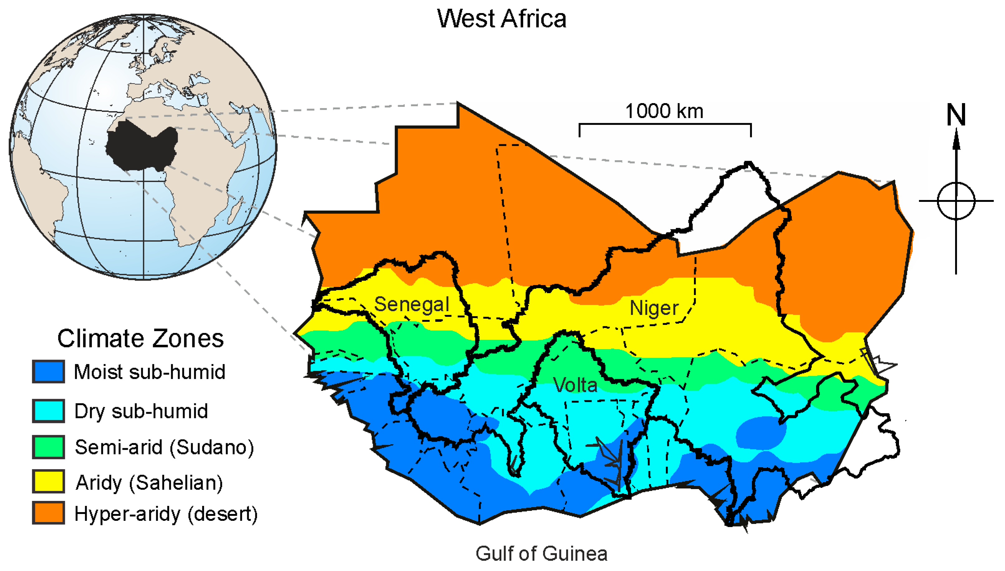
West Africa covers an area of approximately of equivalent to 20% of the total area of Africa lying between longitudes 18° W and 16° E and latitudes 3° N and 28° N (Figure 1). The region is bounded in the west and south by the Atlantic Ocean and in the north by the Sahara Desert. The region’s most important highlands include the Guinea Highlands (including the Fouta Djallon, Guinea), which is the source of many rivers (e.g., Niger, Senegal, Gambia); encompassing parts of Guinea, Sierra Leone, northern Liberia, as well as northwestern Côte d’Ivoire; the Jos Plateau in Nigeria; Mandara Mountains, the source of the Benue river in southeastern Nigeria. The most significant river is the Niger, the fifth largest river in the world and second in Africa, which drains an area of 2 million km2. Other important rivers in the region are the Gambia, Senegal, Comoe, and Volta.
The region is partitioned into sub-climatic zones using the K-means clustering algorithm. As suggested by Andam-Akorful et al. [24], this reclassification of the climatic zones considering their annual rainfall amounts to maintain consistency with the general African sub-climatic classification suggested in by [25]. Thus, the climatic zones are classified as hyper-arid (HA) in the north, arid, semi-arid (SA), dry sub-humid (DSH) and moist sub-humid (MSH) in the south (see Figure 1) the hyper-arid sub-region coincides with the desert area; arid, Sahel; semi-arid, Sudanian; Guinean, the moist and dry sub-humid areas [24]. West African rainfall is highly variable leading to the region experiencing recurrent droughts and floods.
2.2. Datasets
2.2.1. ARCv2 Rainfall
ARCv2 is a revised version of Climate Prediction Center’s (CPC) African Rainfall Climatology (ARC), which provides Africa specific precipitation from 1983 onwards. This product generates fields based on a subset of source data used in the Rainfall Estimate version 2 (RFE2) algorithm at a spatial resolution of 0.1° [26]. ARCv2 input dataset consist of input data from a 3-hourly geostationary infrared (IR) sensor centered over Africa by the European Organization for the Exploitation of Meteorological Satellites (EUMETSAT) and the Global Telecommunication System (GTS) gauge observations. Daily data retrieved from [27] were aggregated to monthly fields at a spatial resolution of 0.25°.
The product was chosen due to its reasonable performance over WA compared to other contemporaneous datasets, such as TRMM, PERSIANN, TAMSAT, and CMORPH [28]. Additionally, it is available from 1983, providing enough data for long-term studies. Note that, the ARCv2 rainfall fields are, however, not available from January 1979 to December 1982. Thus, in Appendix A we used a dedicated network to extend its records to 1979 using rainfall estimates for the Noah driven GLDAS version 2 (V2) land surface model [2], as well as, ENSO and Atlantic Niño indices. The predicted rainfall series showed a strong agreement with the original series over their common overlapping periods (see Table A1 and Figure A1).
2.2.2. ERA-Interim Data System
In order to model response of TWS to evapotranspiration and temperature changes, instantaneous moisture flux (equivalent to evapotranspiration [29]) and land surface air temperature (LSAT) fields were retrieved from ERA-Interim data system. Additionally, precipitation () minus evaporation (), also known as net-precipitation, derived from the atmospheric water budget [24] was used to further characterize TWS response to atmospheric moisture conditions over the region, while soil moisture, also obtained from ERA-Interim was used to model land surface moisture conditions. The datasets were all obtained at a gridded spatial resolution of 0.25° and a monthly temporal interval from [30]. The motivation to predominantly select ERA-Interim reanalysis data for this study is due to its long-term consistency [31].
2.2.3. GLDAS-Noah Version 2
Additionally, total soil moisture (the sum of all layers), canopy and snow storages from GLDAS-Noah [2] in its Version 2 (V2) was also used to validate the result of the ANN predicted TWS, we named it TWC (total water content). GLDAS-2 datasets consist of 0.25°-by-0.25° gridded data, covering the period from 1948 to 2010. The temporal resolution for the GLDAS products is 3-hourly, where monthly products are generated through temporal averaging of the 3-hourly products. The data was retrieved from [32].
2.2.4. Climate Indices
The Bivariate ENSO Time series (BEST, [33]), which is derived from Niño 3.4 and Southern Oscillation Index (SOI) was used to model the response of WA to the ENSO phenomenon. The BEST index combines the atmospheric (SOI) and oceanic (Niño 3.4) components of the ENSO processes into a single field, and thereby, provides a more realistic characterization of the phenomenon. Furthermore, the Atlantic Equatorial Mode, also known as the Atlantic Niño [34], which modulates inter-annual rainfall over the region through the West African Monsoon (WAM) winds [35] was also used to simulate the regional oceanic-atmospheric circulation processes that drive precipitation patterns from the Gulf of Guinea. Finally, the time series of global temperature anomalies were also used to simulate the effect of global warming on TWS variability over the region as the droughts in the late 20th century have been linked to rising temperatures globally.
2.2.5. GRACE Fields
GRACE-derived TWS were computed at a spatial resolution of 1°-by-1° using level 3 products [36], from the three major processing centers—the Center for Space Research (CSR), Jet Propulsion Laboratory (JPL), and the GeoForschungsZentrum (GFZ). The monthly fields were scaled [36], and missing months in the GRACE series were obtained through a bilinear interpolation algorithm. GRACE solutions from the different centers (CSR, GFZ, JPL) present differences due to the unique processing methodologies of respective agencies [37]. In order to obtain of optimal estimates, Sakumura et al. [38] suggested the use of the simple average of the solutions from the different centers. However, since the respective products perform differently in different parts of the world, an uncertainty-based weighting of the ensemble product will offer a more equitable solution [39]. In this study, a different approach which utilizes uncertainty-based weighting is proposed to build an ensemble model. To this end, the Three-Cornered-Hat (TCH) was employed to evaluate the uncertainties of estimates from the different centers in the absence of any reference data. Details are provided in [39] and MATLAB® (The MathWorks, Inc., Natick, MA, USA) scripts are available under request to the authors. The uncertainties were used as weights in the realization of the ensemble model using the expression:
where is the time-dependent normalized weight based on the uncertainties , as obtained from the TCH, expressed as:
Additionally, with the knowledge in the uncertainties within the respective series, the signal-to-noise-ratio (SNR) of each product is computed as a ratio of the RMS to the noise estimate. The purpose of this metric is to assess the amplitude of the TWS field concerning the uncertainties in order to gain a better understanding of the amount of “contamination” within GRACE-derived TWS.
We furthered expressed TWS fields in terms of TWS changes (TWSC, i.e., fluxes) using numeric differentiation using the central derivative operator as:
where is the month. This filter is important in order to compare the TWS with other fluxes, or, in our case, use other fluxes (e.g., rainfall) to backcast TWSC. We also will backcast TWS for comparison with previous works [21].
2.3. Methods
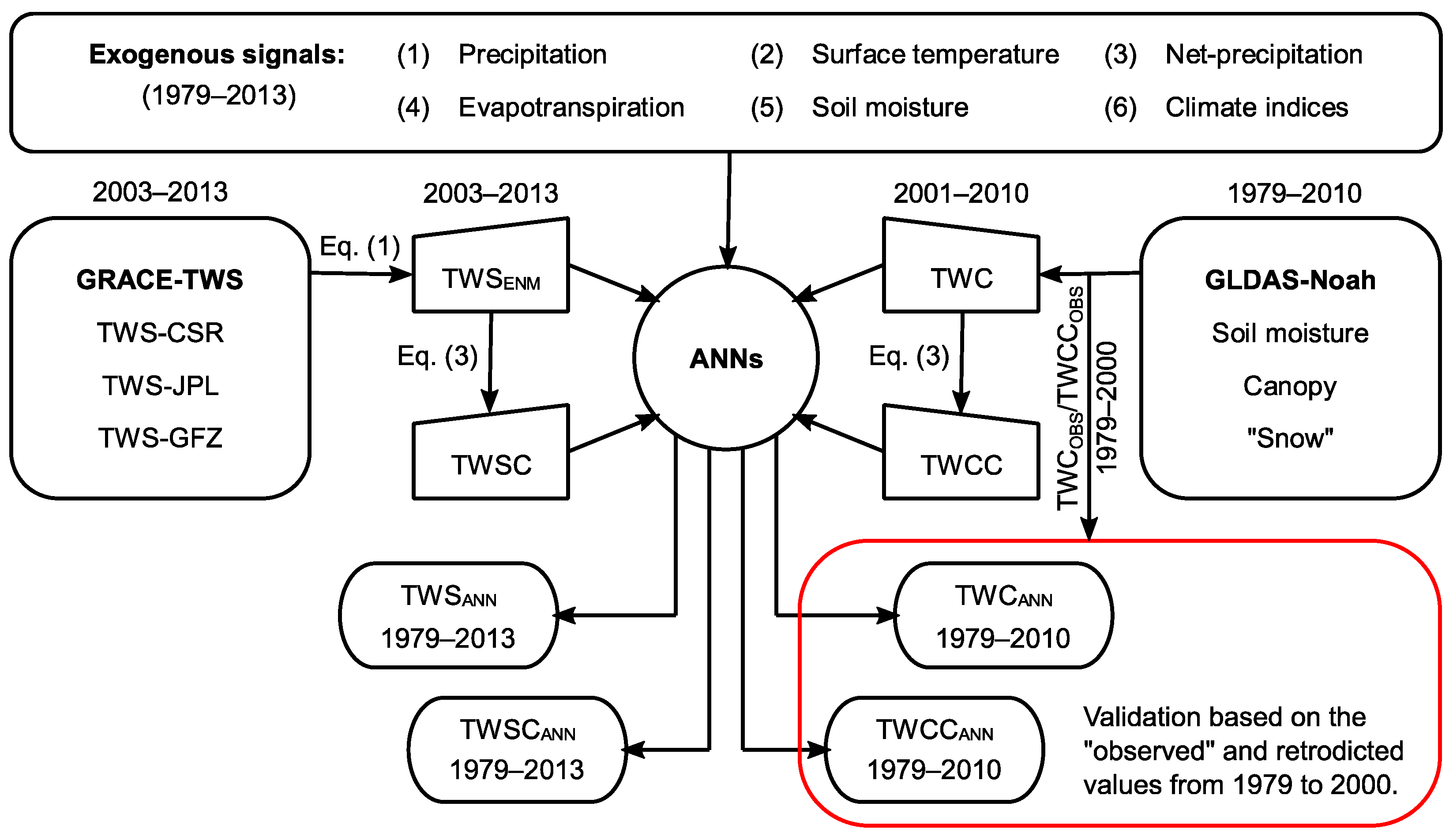
The methodology presented in the next subsections are summarized in Figure 2. First, we constructed a robust time-series for TWS (TWSENM), considering the products computed from the solutions provided by CSR, GFZ, and JPL (see Section 2.2.5). Second, the artificial neural network was considered in a two-fold experiment. Simulation of TWS (TWC) from our preferred hydrological model is used in a “closed-loop” simulation to assess the quality of the extended TWS series from 2003 to 1979 (Section 2.3.1). Third, the outputs from the artificial neural network are validated using the metrics presented in Section 2.3.2.
Due to the lack of long records for the purposes of evaluation, the backasting approach was further validated by designing a similar system to reconstruct TWC from the Noah V2 LSM, which is endowed with long-term data series. This network was trained to predict TWC from 2001 to 2010, after which it was used to backcast TWS from 2010 to 1979. Records from 1979 to 2000 from the reconstructed and the original datasets was then used to validate results from the ANN (Figure 2).
2.3.1. Reconstruction of GRACE-Derived TWS/TWSC
For this study, the Neural Network with eXogenous Inputs (NARX), which is suitable for modeling the nonlinear system was used in the design of the network. It is a dynamic neural network and contains recurrent feedback from several layers of the network to the input layer [40]. A NARX network predicts a signal by regressing the previous values of the output signal and previous values of an independent (exogenous) input signal. Mathematically, a NARX network is expressed as [40]:
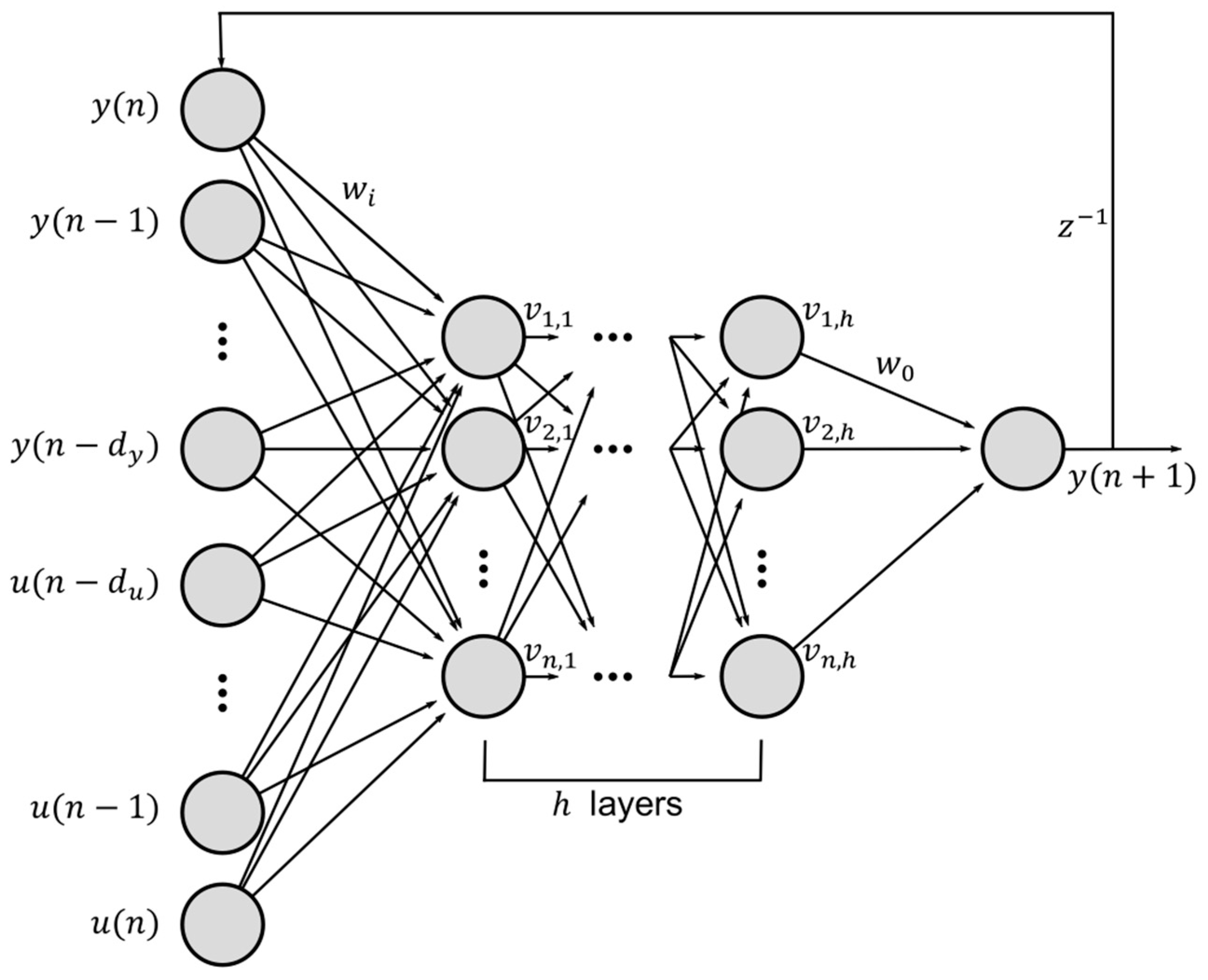
where is the signal to be predicted, are the independent exogenous input signal at a time discreet time step , and is the input and the output delay, and is the transfer function (normally unknown and can be approximated). A NARX architecture is shown in Figure 3 with one time series as input and another as output. In Figure 3, is the discreet time step, is the number of hidden layers, is the weight of input layer, is the weight of the output layer, and is the parameter of the -th layer.
Our backcasting model employed 16 hidden layers and calibrated with a Bayesian regularization back propagation learning algorithm. Furthermore, the sigmoid transfer function was used. The exogenous signals consisted of the several fields, including: rainfall, evapotranspiration, land surface temperature, soil moisture, net-precipitation (P − E) from the atmospheric and terrestrial water budget approaches, and climate indices (BEST and AEM). All the gridded datasets, apart from the GRACE were resampled to a spatial resolution of 0.25° from 1979 to 2013 (34-year period).
Upon readying all needed exogenous variables, 2003 to 2013 was selected as the training period. The trained network was then used to reconstruct TWS from 1979 to 2013. In the designing the network, 70% of the data was used for training, whereas 15% for validation and to stop training before overfitting; and 15% for testing (used as independent data). Additionally, GRACE-derived TWS solutions covering the year 2002 were used to validate the results obtained from the ANN. The same experiment was performed for TWSC, that is, using flux (TWSC) rather than storage (TWS). The resulting solutions from the ANN were smoothed with a discrete cosine transform based smoothing algorithm [41]. We used the Neural Network Toolbox [42] of MATLAB® and the script is available under request to the authors.
To further validate the GRACE estimates in the face of limited data, a similar neural network was created for the GLDAS-Noah simulated total water content (TWC, a combination of all soil moisture layers and vegetation canopy water) data, which is endowed with a long-term series. This network was trained with similar exogenous variables as that of the GRACE-derived TWS (Figure 2) over a 10 year period, that is, 2000 to 2010. The network was then used to predict Noah-derived TWC estimates from 1979 to 2010, and the results compared to the original dataset over the period 1979 to 1999. Like for GRACE data (TWS and TWSC), we performed the same training however for TWCC (i.e., flux after applying the temporal derivative for TWC). This was necessary in order to validate the retrodicted results over the time period of 1979–2000 (for GLDAS-Noah).
2.3.2. Validation Metrics
All backcasted series (ARCv2, GRACE-derived TWS, and Noah) were all evaluated using four validation metrics, which included, the coefficient of determination (); mean error (ME); root mean square error (RMSE); and the Nash-Sutcliffe efficiency coefficient (NSE).
The coefficient of determination allows the quantification of the common information content between observed and backcasted series and is given by:
where is the backcasted value at an epoch, and is the original value. The range of lies between 0 (no correlation) and 1 (perfect fit), which describes how much of the observed dispersion is explained by the backcasting. The drawback of when considered alone is that, a model with large positive/negative bias may still show a good correlation and thus, require the additional consideration of other metrics such as ME and RMSE.
Alternatively, the NSE is given as:
NSE ranges between and 1, 1 signifying a perfect fit (the backcasted and original estimates agree in mean, amplitude, and phase), whereas an efficiency lower than zero indicates that the mean value of the observed time series would have been a better predictor than the model (the ANN in this case).
Like , NSE is not very sensitive to model over- or underprediction, especially during dry epochs [43]. RMSE is obtained as:
Finally, ME is given as
In Equation (8), if dividing the residuals by the observed field would provide the mean bias error (MBE).
3. Results
3.1. The Ensemble GRACE-TWS Fields
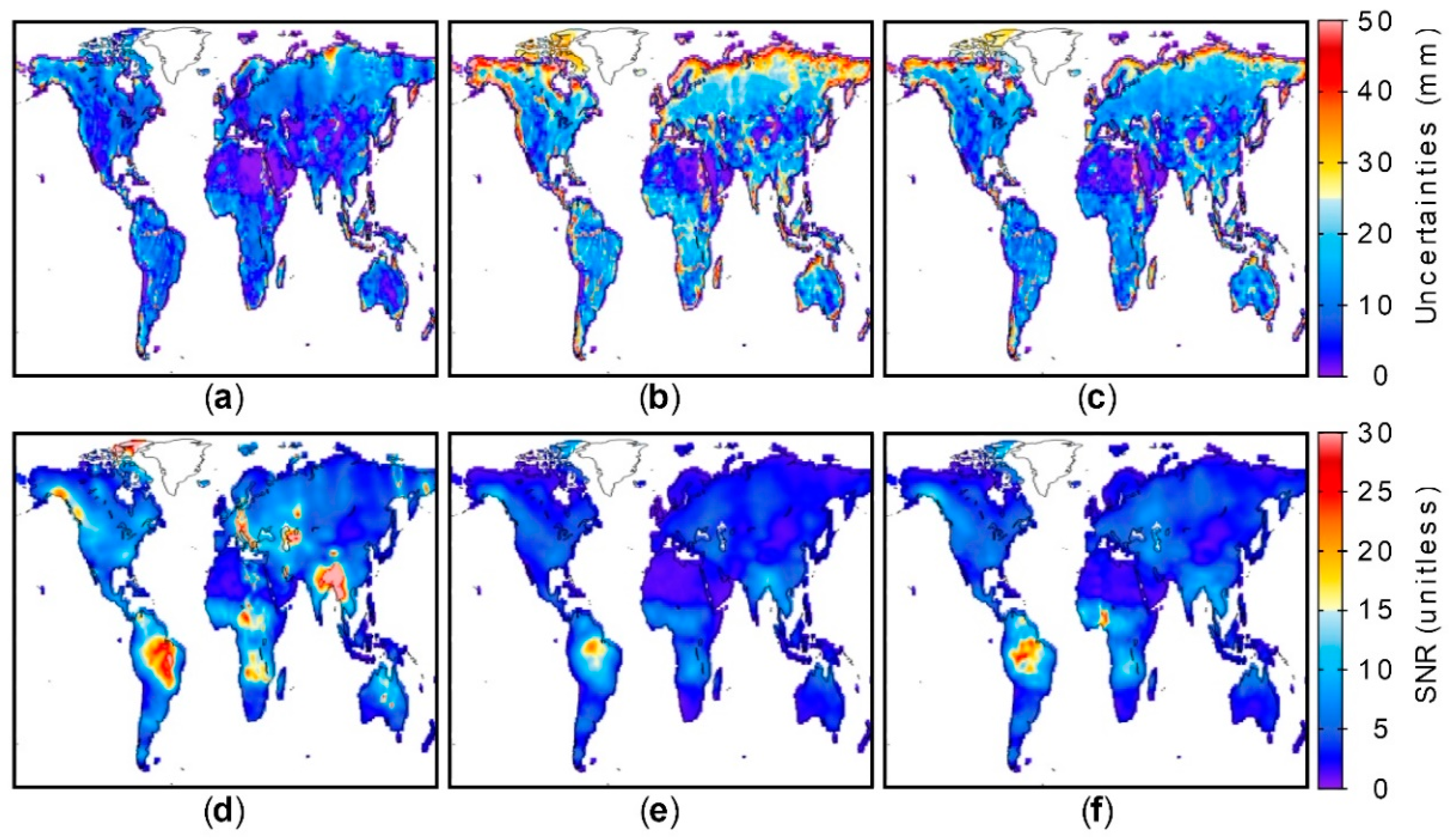
Figure 4 illustrates the spatial distribution of the uncertainties and SNRs based on TCH method. It is evident that CSR estimates present lower uncertainties relative to GFZ and JPL (compare Figure 4a–c, respectively).
The spatial distribution of the uncertainties shows high estimates along the coastlines, especially around North America and Russia, whereas low estimates are observed in arid regions, for example, the Sahara and Gobi deserts (Figure 4a–c).
On the other hand, high SNRs are observed in places with high amplitudes in TWS, such as, the Amazon basin (Figure 4d–f). Again, CSR (Figure 4d) shows the best performance as expressed by SNR values.
Table 1 presents the distribution of the magnitudes of uncertainties and SNRs, expressed in percentages over landed areas globally with 91.5% of its estimates falling within 0–20 mm of the noise. Similarly, CSR presents slightly higher SNRs as opposed to the other two products.
The comparisons between ensemble models, constructed with simple averaging, that is Equation (1) without weights, and uncertainty-based weighting, that is Equation (1) considering the weights given by Equation (2), are given in Table 2.
About 97% of the cells distribution, present uncertainties lower than 10 mm in the weighted model, ENMTCH, as opposed to 87% in ENMAVE (Table 2). Although both products have higher SNRs than the original series from the processing centers, the weighted product (ENMTCH) indicate higher SNRs compared to the averaged one (ENMAVE). Whereas approximately, 86% of the cells in ENMAVE have SNRs lower than 20, only about 64% of those of ENMTCH fall within the same range, while significant 27% of the grids have their SNRs between the 20–40 range, in contrast to the 11% of ENMAVE.
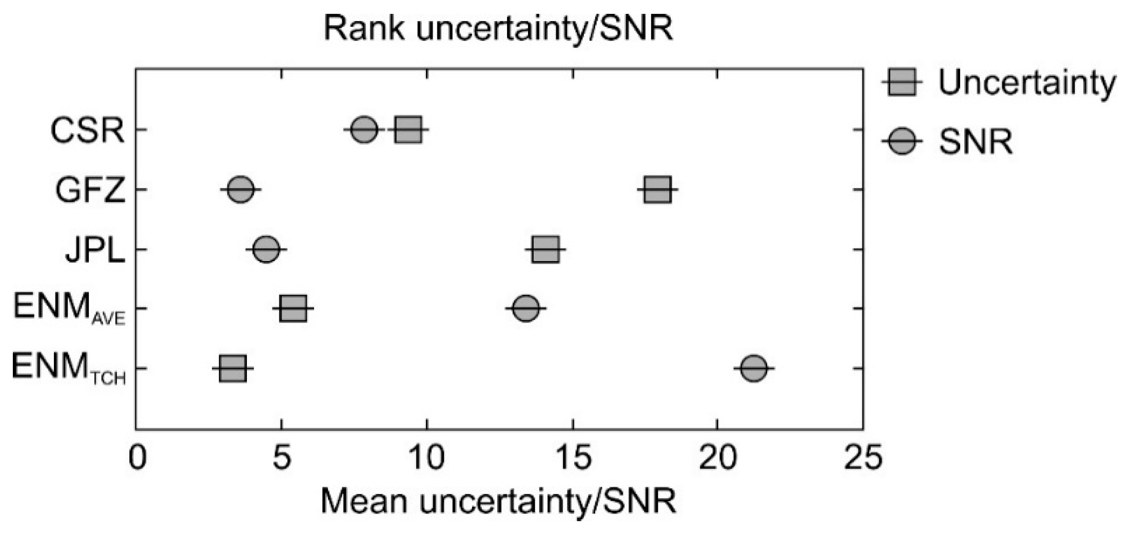
The multiple comparison procedure (MCP) [44,45] was also applied to evaluate the statistical differences between the original products and the two ensemble models, as well as, a statically based ranking of the means of the different datasets. The results of the MCP confirm that, the mean uncertainties in the combined models are lower than the original series (Figure 5). Again, the TCH weighted model outperforms the averaged one both in terms of uncertainties and SNRs, as shown in Figure 5. (Note, low values of mean uncertainties better the model, conversely, higher values of SNRs imply better the model.)
The procedure ranks the original products in the following descending order: CSR, JPL, and GFZ for both, uncertainties and SNRs. It must be noted here that, this is not to be used as a basis of choosing one product over the other, as many studies, including our own, indicate that products from the different processing centers essentially yield similar results. However, the use of a combined product, especially weighted by uncertainties is strongly recommended as shown the current study, in agreement with Sakumura et al. [38].
3.2. Confirmatory Study Based on Noah-Derived TWCC Prediction
In Figure 6, the results of the confirmatory validation by comparing ANN predicted Noah TWC and the observed estimates are presented.
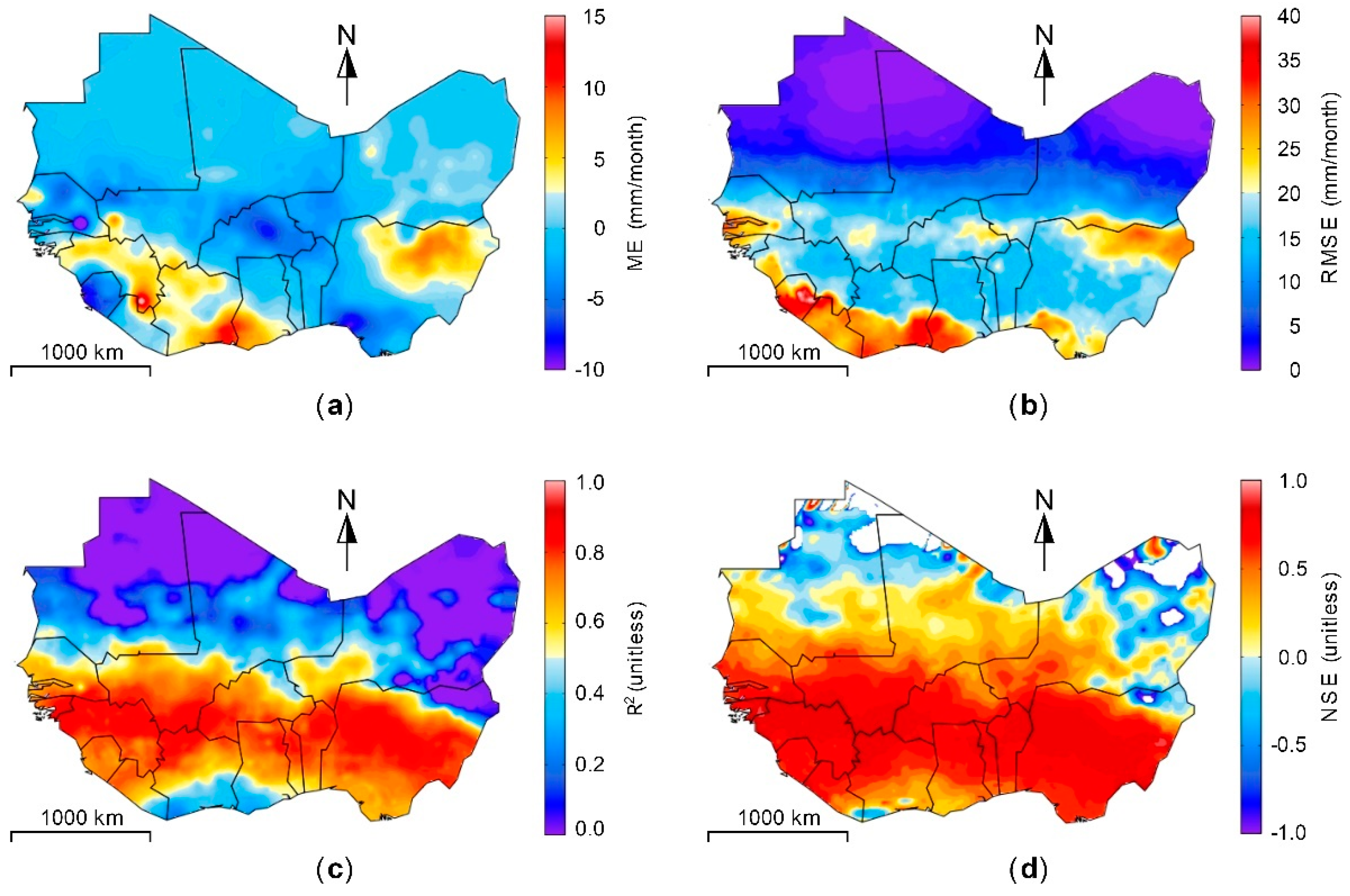
Generally, the more humid south (apart from the very humid southwest) exhibited negative biases (Figure 6a), while the mid-latitude areas presented moderate to high overestimations. The hyper-arid areas in the north presented low RMSEs (Figure 6b), mostly less than 5 mm. The RMSEs for most other areas generally ranged between 10 to 20 mm, while relatively large values were found over wetter regions in south WA, as well as parts of the eastern section.
Correlations between the two datasets (predicted versus the actual) were high in the relatively humid south () in contrast to the low correlation coefficients in the dry north (Figure 6c). At the high latitudes, some areas even presented negative correlations, indicating a likely weak performance of the network in the desert areas. The weak performance in this area is however of negligible effect to analysis performed in this study as most of the TWS variance occur from the Sahelian area down to the coastal south. Similarly, NSE, as shown in Figure 6d indicate high performance in the south relative to the desert areas in the north.
Table 3 indicates high skill scores for all spatial averages. Thus, it can be concluded that, the ANN estimates are of high quality and can be used to adequately characterize spatial and temporal patterns in freshwater reserves over WA. (This is presented in the next, Section 3.3.)
3.3. Evaluation of Backcasted GRACE-Derived TWSC
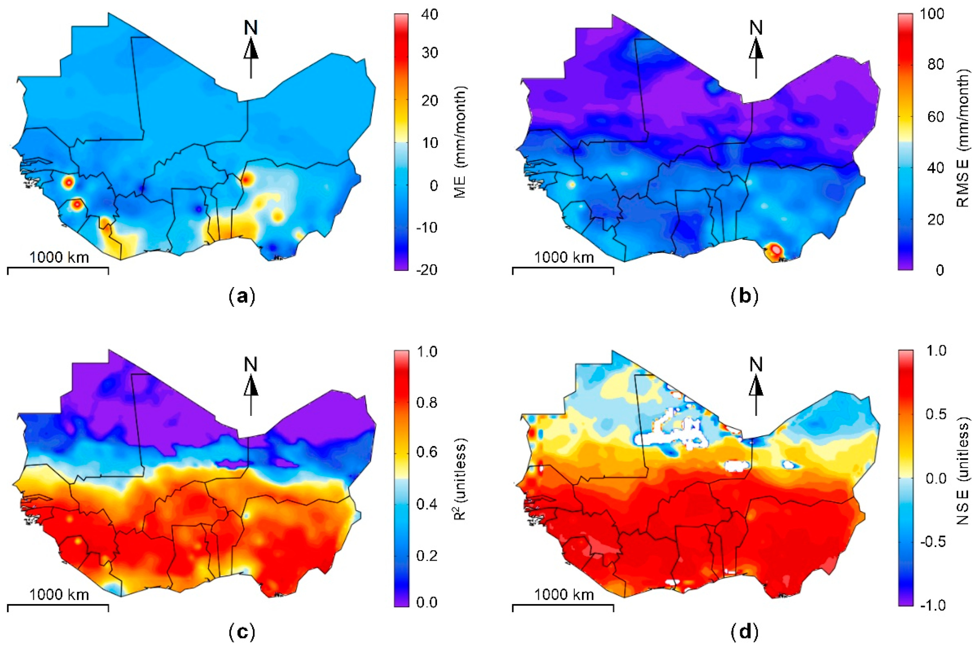
The performance skills of the GRACE-derived TWSC are illustrated in Figure 7.
The MEs (Figure 7a) range from −20 to 40 mm/month across WA, although values range from approximately −10 to 10 mm/month in most areas. The RMSEs (Figure 7b) are lowest over the Sahara (≤15 mm/month), while the areas south of the Sahara generally present values between 20 and 50 mm/month. The highest RMSEs were found around the Niger Delta, with values around 100 mm/month.
The coefficients of determination (Figure 7c) indicate low correlations in the Sahara (R2 ≤ 0.5), whereas the values in the Sahel and below are greater than or equal to 0.6. The spatial patterns of NSEs are like those of the R2, with worst efficiencies being observed in over the Sahara, and values greater than or equal to 0.5 occurring from the Sahelian areas to the more humid south (see Table 4 and Figure 1).
All major basins and sub-climatic areas as presented in Table 4 show high skill score in all four metrics, apart from the Sahara’s NSE score (0.26). The highest RMSE was observed in the humid area, whereas the lowest was expectedly recorded for the Sahara.
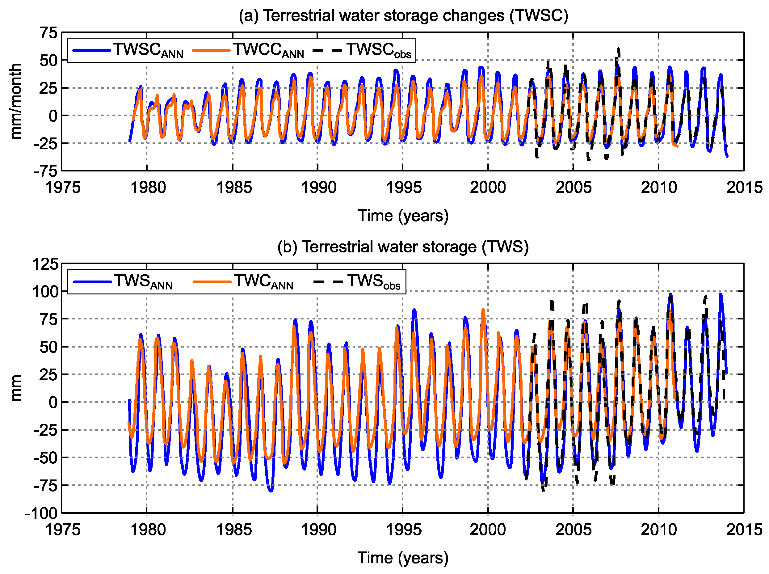
Figure 8a is a plot of the WA spatially-averaged estimates of TWSCANN, TWSCobs, and TWCCNoah.
The strong agreement between the three series is evident. It is worth mentioning here that, TWCCNoah was not considered as an exogenous data input during the training of the ANN used to retrodict GRACE-TWSC. Its strong agreement with the reconstructed GRACE series therefore, indicates robustness of the predicted estimates over the region.
Similarly to TWSC, Figure 8b presents spatially-averaged time series of GRACE-derived TWS estimates from the ANN (TWSANN) as well as the observed (TWSobs) and Noah (TWCNoah) estimates. We performed this in order to compare with previous results [21,23]. The three series show a strong agreement over their respective overlapping periods. TWSANN presents a high correlation with TWSobs with an R2 of 0.90 and an RMSE of 12.92 mm. The TWSANN signal amplitudes between 2003 and 2007 are slightly lower than those of TWSobs, however, the converse is observed from 2008 onwards. With respect to TWSNoah, an R2 of 0.89 was obtained, indicating a high correlation. The Noah estimates tend to present a wet bias throughout the period of data availability (1979 to 2010). This seems to be because model-based estimates of TWS are less variable than GRACE-derived TWSC primarily due to the absence of underground water storage as well as surface water reservoir storage.
In Figure 8b it seems that inter-annual variations exist for the stored water through the decades. Thus, in Table 5 it is presented the long-term trends for the series considering different time periods.
Generally, the backcasted TWS over the region presented an upward linear trend of 1.04 ± 0.21 mm/year from 1979 to 2013 (34-year period), whereas TWCNoah indicated a positive trend of 0.76 ± 0.19 mm/year (Table 5). The linear trend from 2007 to 2013 is especially strong with a value of 4.36 ± 2.40 mm/year, while 1979 to 2006 presented a value of 0.67 ± 0.28 mm/year. All statistical measures were computed at a 95% confidence level.
4. Discussion
One of the main goal of this experiment was to attempt to assess the quality of backcasted GRACE-derived TWS over WA. We considered a “closed-loop” simulation by using synthetic TWSC (i.e., TWCC) predicted by a land surface model, GLDAS-Noah V2, since it covers the entire period of study. A period equivalent to the GRACE observation were used to generate an artificial neural network-based learning machine (ANN NARX) and then retrodict the TWCC till 1979. The network was trained to simulate Noah TWCC signals from 2003 to 2010 over WA, based on their physical nonlinear relationships with seven hydro-climatic variables (rainfall; evapotranspiration; land surface air temperature; net-precipitation; soil moisture; ENSO index; and global temperature anomaly). This was necessary in order to validate the ANN NARX. Overall, the results of this network presented similar spatial accuracies as that of GRACE, whereas the spatially-averaged TWCC presented ME, RMSE, NSE and of 0.13 mm/month, 5.01 mm/month, 0.91, and 0.93, respectively (Table 3). Furthermore, considering the main river basins over WA and the climate zones (cf., Figure 1), the errors are within GRACE-derived TWS [38,39]. There is some overestimation over moist sub-humid areas (Figure 6a) although NSE values shows reasonable performance. Yet, the ANN method seems to be robust to adequately reconstruct GRACE-derived TWSC estimates over WA as shown by the simulation.
Following this, the second goal was to retrodict the actual GRACE-derived TWSC to 1979 using a similar network. Firstly, an ensemble model of GRACE-derived TWS was created using the data from the three primary processing centers (CSR, JPL, and GFZ). In this regard, we applied the TCH method to independently estimate uncertainties in GRACE-derived TWS. The overall uncertainties estimated for the individual processing centers show that CSR delivered the lowest values. This is somewhat in agreement with previous studies [38,39], which found CSR providing the lowest noises among three processing centers. The computed uncertainties were subsequently used as weights in creating an ensemble TWS model from the original series, as well as, another combined model obtained through simple averaging. The weighted ensemble product, when compared to the original and the averaged datasets presented lower noise estimates and higher SNRs (Table 1 and Table 2), indicating an improvement in the TWS solution. This improvement in the ensemble series using weights contrasts with the results provided in Ref. [38].
Following this, the improved product was used in the reconstruction of GRACE TWSC (TWS was converted to TWSC by means of Equation (3)) retrodicted from 2013 to 1979 (34-years period) using an ANN NARX. Figure 8a depicts the averaged series for WA, which shows an overall agreement with observed TWSC with ME, RMSE, NSE, and of 0.05 mm/month, 6.98 mm/month, 0.91, and 0.91, respectively. Despite the differences in the length of the comparisons, the results of a “closed-loop” simulation (Noah-TWCC) and those for actual data (GRACE-TWSC) show consistency for the entire region and its sub-domains (compare Table 3 and Table 5). Furthermore, the use of TWSC shows relatively low NSE values in comparison with previous studies that adopted TWS [12,21,23], known that there are differences in the datasets, time span, study region, etc.
To support the above discussion that TWSC is a better candidate to be predicted than TWS an ANN NARX was trained to predict GRACE-TWS with the same hydro-climatic variables. Similarly, the ANN NARX predicted GRACE-derived TWS series (TWSANN), showed strong agreement with the original GRACE data, presenting similar trends over their overlapping periods (Figure 8b). The results, upon validation showed high skill scores, mostly in areas south of the Sahara Desert, but low performance in the desert due to the very low amplitudes in signals. The coefficient of determination and NSE coefficient values obtained for areas south of the Sahara were mostly greater or equal to 0.6 and 0.5, respectively, while RMSEs ranging from 20 mm to 50 mm were predominant. Spatially-averaged series for major basins and sub-climatic zones, as well as, the whole of WA itself presented median RMSE, NSE and of 11.83 mm, 0.76 and 0.89, respectively. This is somewhat in agreement with the findings presented in [12], thought different scenarios. Interesting, Figure 8a shows a better agreement between GRACE-TWSC with Noah-TWCC in comparison with the results depicted in Figure 8b, which shows GRACE-TWS and Noah-TWC. That means TWSC over WA mainly reflects fluctuations in soil moisture while TWS still have some memory effect, mainly in the groundwater compartments.
As mentioned in the Section 1 (Introduction), so far no one appear to have assessed ANN considering a “closed-loop” simulation. Thus, the importance of results using such algorithm lies both to validate the algorithm in the aim that the errors lie within an acceptable range (e.g., GRACE errors) and to provide long-term series to enable long term studies (e.g., droughts). However, we have not considered and investigated the contribution of desiccation of Lake Chad [46] on the hindcasted TWSC. Furthermore, the regularization of Lake Volta due to the water impoundment must be considered. Sensitivity of the output in ANN to the set of the parameters has not been considered. We just used seven hydro-meteorological variables that could modulate TWSC over WA, however, it is recommended to select inputs one-by-one or several at a time to assess the prediction performance to a set of inputs. Nonetheless, our finds support the use of ANN to extend TWSC series dedicated to long-term studies over West Africa, a data-poor region.
5. Summary
Although GRACE currently offers the most viable option of obtaining reliable estimates of TWS at regional and global scales, its time series is relatively short. For example, it cannot be used to infer the long-term changes in water availability over West Africa since the 1970s. Thus, a data-driven machine learning approach, which involved the use of NARX network was adopted to retrodict the GRACE series to 1979. The network was trained to learn the complex nonlinear relationships between GRACE-derived TWSC and the following hydrological variables: rainfall; temperature; evapotranspiration; net-precipitation; soil moisture, ENSO and Atlantic Niño (Niña) indices; and global temperature anomalies over the period 2003 to 2013. The trained network was subsequently used to backcast TWSC estimates from 2013 to 1979 covering a period of 34 years. Due to the lack of long-term records for the purposes of validation, a similar system was designed to synthesized TWSC (i.e., TWCC since there is no groundwater and surface water storages) from the Noah driven GLDAS land surface model, which is endowed with long-term series in its Version 2. This network was trained to predict TWCC from 2000 to 2010, after which, it was used to backcast TWCC from 2010 to 1979. Records from 1979 to 1999 from the reconstructed and the original datasets were then used to validate results from the ANN NARX.
Overall, the network employed to reconstruct Noah series yielded good spatial accuracies, with the spatially-averaged TWCC estimates presenting median RMSE, NSE and of 8.06 mm/month, 0.76 and 0.88 respectively. Thus, the artificial neural network method proved robust to adequately reconstruct GRACE-derived TWS estimates over West Africa. For the real GRACE data, the reconstructed TWSC series, showed strong agreement with the original GRACE data, presenting similar trends over their overlapping periods. The results, upon validation showed high skill scores, mostly in areas south of the Sahara Desert, but low performance in the desert dues to the very low amplitudes in signals. The spatially-averaged series for major basins and sub-climatic zones, as well as, the whole of West Africa itself, presented median RMSE, NSE, and of 11.83 mm/month, 0.76 and 0.89, respectively. These results agree with those of the “closed-loop” simulation and thereby we can conclude that the NARX network method used here proved robust to adequately reconstruct GRACE-derived TWSC estimates over West Africa.
Author Contributions
V.G.F. conceived and designed the experiments. S.A.A.-A. performed the experiments as part of his PhD thesis and R.D. improved the figures. E.A.-A. contributed with the improvements in the methods and study area. V.G.F., S.A.A.-A., R.D., and E.A.-A. analyzed the data, contributed to the discussions, and wrote the paper.
Funding
This research was funded by National Natural Science Foundation of China, grant number 41574001.
Acknowledgments
Vagner G. Ferreira acknowledges the support from the National Natural Science Foundation of China (Grant No. 41574001) and the Fundamental Research Funds for the Central Universities (Grant No. 2015B21014). We thank all the dataset providers used in this study as described in Section 2.1. We are also grateful for the comments and suggestions of the editors and reviewers.
Conflicts of Interest
The authors declare no conflict of interest.
Appendix A
The rainfall fields from ARCv2 are not available from January 1979 to December 1982, hence, an ANN NARX was trained to provide data from that period, using rainfall fields from the Noah, as well as, the BEST series as exogenous data inputs in order to generate enough data to cover the entire period of this study. The rainfall fields from Noah were used due to their relatively fine resolution, compared to those of Global Precipitation Climatology Centre (GPCC). Additionally, they were found to be very consistent with the GPCC rainfall estimates. The training period spanned 1990 to 2010, while the rainfall estimates were reconstructed from 1979 to 1991.
The reconstructed estimates from 1983 to 1989 were then validated with the original ARCv2 data using four metrics described in Section 2.3.2. Table A1 presents the metrics of spatially-averaged estimates over basins and sub-climatic zones, as well as, WA itself.
For all spatially-averaged rainfall estimates, the ANN results generally show a strong correlation, with , with the Niger basin and the dry sub-humid region presenting the highest values, , while the Senegal basin and Sudanian region presented the lowest (). Similarly, high NSE values were obtained for most of the areal averages (), however, the areas within the Sahara showed a poor performance, which is to be expected over a hyper-arid. Additionally, the ME and RMSE values were generally larger in the more humid areas, compared to the drier places; except for the humid zone, all areal averages showed underestimations. The apparent poor performance in the relatively dry areas is generally in consistence with Awange et al. [28] who demonstrated that, rainfall estimates over dry areas present lower uncertainties, compared to estimates in more humid areas, due to the low amplitudes of the signals. The SNRs however, show a poor performance in these dry areas.

Table A1.
Area-averaged statistics for backcasted ARCv2 rainfall estimates over river basins and sub-climatic zones (see Figure 1 for the regions).
Table A1.
Area-averaged statistics for backcasted ARCv2 rainfall estimates over river basins and sub-climatic zones (see Figure 1 for the regions).
| Region | ME (mm/month) | RMSE (mm/month) | NSE | R2 | |
|---|---|---|---|---|---|
| Basin | Niger | 2.76 | 13.10 | 0.90 | 0.92 |
| Senegal | 1.56 | 16.50 | 0.82 | 0.83 | |
| Volta | 5.36 | 23.01 | 0.83 | 0.84 | |
| Climate zones | Humid | −2.64 | 30.90 | 0.82 | 0.88 |
| Dry sub-humid | 4.65 | 20.66 | 0.90 | 0.92 | |
| Sudanian | 4.81 | 18.47 | 0.89 | 0.83 | |
| Sahelian | 3.76 | 13.90 | 0.76 | 0.84 | |
| Sahara | 1.13 | 4.92 | 0.26 | 0.92 | |
| WA | 2.21 | 11.00 | 0.89 | 0.92 | |
Figure A1 presents the results of the extended ARCv2 rainfall estimates from 1983 to 1979, compared to original series.
Figure A1.
Validation of artificial neural network-based learning machine (ANN NARX) predicted African Rainfall Climatology (ARC) v2 rainfall data. (a) Mean error—ME; (b) Root-mean-square error—RMSE; (c) Coefficient of determination—; and (d) Nash-Sutcliffe efficiency coefficient—NSE.
Figure A1.
Validation of artificial neural network-based learning machine (ANN NARX) predicted African Rainfall Climatology (ARC) v2 rainfall data. (a) Mean error—ME; (b) Root-mean-square error—RMSE; (c) Coefficient of determination—; and (d) Nash-Sutcliffe efficiency coefficient—NSE.

It is apparent that estimates in the relatively humid south have higher mean positive bias (Figure A1a). The maximum mean bias was positive 4.6 mm/month, while −4.8 mm/month was the largest underestimation. Similarly, the highest RMSEs (≤55 mm/month) were observed along the coast, decreasing progressively to the relatively dry north as shown in Figure A1b. The backcasted and observed rainfall estimates showed high correlations in the mid-latitudinal areas, with low values along the southwestern coast and the dry north. Correlations, especially at the extreme northwest and northeast were found to be particularly low. It is worth noting that, this area is part of the hyper arid Sahara Desert where there is little or no precipitation throughout the year (Figure 1). Similarly, the estimates in the mid-latitude areas show the highest performance as indicated by the NSE while the Sahara regions exhibit the lowest skills.
References
- Xie, H.; Longuevergne, L.; Ringler, C.; Scanlon, B. Calibration and evaluation of a semi-distributed watershed model of sub-Saharan Africa using GRACE data. Hydrol. Earth Syst. Sci. Discuss. 2012, 9, 2071–2120. [Google Scholar] [CrossRef]
- Rodell, M.; Houser, P.R.; Jambor, U.; Gottschalck, J.; Mitchell, K.; Meng, C.-J.; Arsenault, K.; Cosgrove, B.; Radakovich, J.; Bosilovich, M.; et al. The Global Land Data Assimilation System. Bull. Am. Meteorol. Soc. 2004, 85, 381–394. [Google Scholar] [CrossRef] [Green Version]
- Schuol, J.; Abbaspour, K.C. Calibration and uncertainty issues of a hydrological model (SWAT) applied to West Africa. Adv. Geosci. 2006, 2, 137–143. [Google Scholar] [CrossRef]
- Rodell, M.; Famiglietti, J.S.; Wiese, D.N.; Reager, J.T.; Beaudoing, H.K.; Landerer, F.W.; Lo, M.-H. Emerging trends in global freshwater availability. Nature 2018, 557, 651–659. [Google Scholar] [CrossRef] [PubMed]
- Forootan, E.; Kusche, J.; Loth, I.; Schuh, W.-D.; Eicker, A.; Awange, J.; Longuevergne, L.; Diekkrüger, B.; Schmidt, M.; Shum, C.K. Multivariate Prediction of Total Water Storage Changes Over West Africa from Multi-Satellite Data. Surv. Geophys. 2014, 35, 913–940. [Google Scholar] [CrossRef] [Green Version]
- Becker, M.; Meyssignac, B.; Xavier, L.; Cazenave, A.; Alkama, R.; Decharme, B. Past terrestrial water storage (1980-2008) in the Amazon Basin reconstructed from GRACE and in situ river gauging data. Hydrol. Earth Syst. Sci. 2011, 15, 533–546. [Google Scholar] [CrossRef]
- de Linage, C.; Famiglietti, J.S.; Randerson, J.T. Statistical prediction of terrestrial water storage changes in the Amazon Basin using tropical Pacific and North Atlantic sea surface temperature anomalies. Hydrol. Earth Syst. Sci. 2014, 18, 2089–2102. [Google Scholar] [CrossRef]
- Yin, W.; Hu, L.; Han, S.; Zhang, M.; Teng, Y. Reconstructing Terrestrial Water Storage Variations from 1980 to 2015 in the Beishan Area of China. Geofluids 2019, 2019, 3874742. [Google Scholar] [CrossRef]
- Wilby, R.L.; Abrahart, R.J.; Dawson, C.W. Detection of conceptual model rainfall—Runoff processes inside an artificial neural network. Hydrol. Sci. J. 2003, 48, 163–181. [Google Scholar] [CrossRef]
- Mukhopadhyay, A. Application of visual, statistical and artificial neural network methods in the differentiation of water from the exploited aquifers in Kuwait. Hydrogeol. J. 2003, 11, 343–356. [Google Scholar] [CrossRef]
- Feng, L.; Hong, W. On hydrologic calculation using artificial neural networks. Appl. Math. Lett. 2008, 21, 453–458. [Google Scholar] [CrossRef] [Green Version]
- Long, D.; Shen, Y.; Sun, A.; Hong, Y.; Longuevergne, L.; Yang, Y.; Li, B.; Chen, L. Drought and flood monitoring for a large karst plateau in Southwest China using extended GRACE data. Remote Sens. Environ. 2014, 155, 145–160. [Google Scholar] [CrossRef]
- Sorooshian, S.; Hsu, K.-L.; Gao, X.; Gupta, H.V.; Imam, B.; Braithwaite, D. Evaluation of PERSIANN System Satellite–Based Estimates of Tropical Rainfall. Bull. Am. Meteorol. Soc. 2000, 81, 2035–2046. [Google Scholar] [CrossRef] [Green Version]
- Nourani, V.; Baghanam, A.H.; Adamowski, J.; Gebremichael, M. Using self-organizing maps and wavelet transforms for space–time pre-processing of satellite precipitation and runoff data in neural network based rainfall–runoff modeling. J. Hydrol. 2013, 476, 228–243. [Google Scholar] [CrossRef]
- Goyal, M.K. Monthly rainfall prediction using wavelet regression and neural network: An analysis of 1901–2002 data, Assam, India. Theor. Appl. Climatol. 2014, 118, 25–34. [Google Scholar] [CrossRef]
- Haykin, S.O. Neural Networks and Learning Machines, 3rd ed.; Pearson: London, UK, 2008; ISBN 9780131471405. [Google Scholar]
- Yirdaw-Zeleke, S. Implications of GRACE Satellite Gravity Measurements for Diverse Hydrological Applications. Ph.D. Thesis, University of Manitoba, Winnipeg, MB, Canada, 2010. [Google Scholar]
- Miro, M.E.; Famiglietti, J.S. Downscaling GRACE remote sensing datasets to high-resolution groundwater storage change maps of California’s Central Valley. Remote Sens. 2018, 10, 143. [Google Scholar] [CrossRef]
- Sun, A.Y. Predicting groundwater level changes using GRACE data. Water Resour. Res. 2013, 49, 5900–5912. [Google Scholar] [CrossRef] [Green Version]
- Yang, Y.; Long, D.; Guan, H.; Scanlon, B.R.; Simmons, C.T.; Jiang, L.; Xu, X. GRACE satellite observed hydrological controls on interannual and seasonal variability in surface greenness over mainland Australia. J. Geophys. Res. Biogeosci. 2014, 119, 2245–2260. [Google Scholar] [CrossRef] [Green Version]
- Zhang, D.; Zhang, Q.; Werner, A.D.; Liu, X. GRACE-Based Hydrological Drought Evaluation of the Yangtze River Basin, China. J. Hydrometeorol. 2016, 17, 811–828. [Google Scholar] [CrossRef]
- Mukherjee, A.; Ramachandran, P. Prediction of GWL with the help of GRACE TWS for unevenly spaced time series data in India: Analysis of comparative performances of SVR, ANN and LRM. J. Hydrol. 2018, 558, 647–658. [Google Scholar] [CrossRef]
- Chen, X.; Jiang, J.; Li, H. Drought and flood monitoring of the Liao River Basin in Northeast China using extended GRACE data. Remote Sens. 2018, 10, 1168. [Google Scholar] [CrossRef]
- Andam-Akorful, S.A.; Ferreira, V.G.; Ndehedehe, C.E.; Quaye-Ballard, J.A. An investigation into the freshwater variability in West Africa during 1979-2010. Int. J. Climatol. 2017, 37, 333–349. [Google Scholar] [CrossRef]
- Nicholson, S.E. The Spatial Coherence of African Rainfall Anomalies: Interhemispheric Teleconnections. J. Clim. Appl. Meteorol. 1986, 25, 1365–1381. [Google Scholar] [CrossRef] [Green Version]
- Novella, N.S.; Thiaw, W.M. African Rainfall Climatology Version 2 for Famine Early Warning Systems. J. Appl. Meteorol. Climatol. 2013, 52, 588–606. [Google Scholar] [CrossRef] [Green Version]
- Africa Rainfall Climatology (ARC). ARC Version 2 (ARC2). Available online: ftp://ftp.cpc.ncep.noaa.gov/fews/fewsdata/africa/arc2/bin/ (accessed on 15 March 2015).
- Awange, J.L.; Ferreira, V.G.; Forootan, E.; Khandu; Andam-Akorful, S.A.; Agutu, N.O.; He, X.F. Uncertainties in remotely sensed precipitation data over Africa. Int. J. Climatol. 2016, 36, 303–323. [Google Scholar] [CrossRef]
- Ahn, J.; Hong, S.; Cho, J.; Lee, Y.-W.; Lee, H. Statistical Modeling of Sea Ice Concentration Using Satellite Imagery and Climate Reanalysis Data in the Barents and Kara Seas, 1979–2012. Remote Sens. 2014, 6, 5520–5540. [Google Scholar] [CrossRef] [Green Version]
- European Centre for Medium-Range Weather Forecasts (ECMWF). Interim Reanalysis Data (ERA). Available online: https://apps.ecmwf.int/datasets/data/interim-full-moda/levtype=sfc/ (accessed on 26 April 2015).
- Forootan, E.; Didova, O.; Schumacher, M.; Kusche, J.; Elsaka, B. Comparisons of atmospheric mass variations derived from ECMWF reanalysis and operational fields, over 2003–2011. J. Geod. 2014, 88, 503–514. [Google Scholar] [CrossRef] [Green Version]
- Global Land Data Assimilation System (GLDAS). GLDAS Noah Land Surface Model L4 3 hourly 0.25 x 0.25 degree, V2.0. Available online: https://disc.gsfc.nasa.gov/ (accessed on 10 February 2018).
- Smith, C.A.; Sardeshmukh, P.D. The effect of ENSO on the intraseasonal variance of surface temperatures in winter. Int. J. Climatol. 2000, 20, 1543–1557. [Google Scholar] [CrossRef] [Green Version]
- Lutz, K.; Rathmann, J.; Jacobeit, J. Classification of warm and cold water events in the eastern tropical Atlantic Ocean. Atmos. Sci. Lett. 2013, 14, 102–106. [Google Scholar] [CrossRef] [Green Version]
- Nicholson, S.E. The West African Sahel: A Review of Recent Studies on the Rainfall Regime and Its Interannual Variability. ISRN Meteorol. 2013, 2013, 1–32. [Google Scholar] [CrossRef] [Green Version]
- Landerer, F.W.; Swenson, S.C. Accuracy of scaled GRACE terrestrial water storage estimates. Water Resour. Res. 2012, 48, W04531. [Google Scholar] [CrossRef]
- Bruinsma, S.; Lemoine, J.-M.; Biancale, R.; Valès, N. CNES/GRGS 10-day gravity field models (release 2) and their evaluation. Adv. Space Res. 2010, 45, 587–601. [Google Scholar] [CrossRef]
- Sakumura, C.; Bettadpur, S.; Bruinsma, S. Ensemble prediction and intercomparison analysis of GRACE time-variable gravity field models. Geophys. Res. Lett. 2014, 41, 1389–1397. [Google Scholar] [CrossRef] [Green Version]
- Ferreira, V.G.; Montecino, H.D.C.; Yakubu, C.I.; Heck, B. Uncertainties of the Gravity Recovery and Climate Experiment time-variable gravity-field solutions based on three-cornered hat method. J. Appl. Remote Sens. 2016, 10, 015015. [Google Scholar] [CrossRef] [Green Version]
- Ardalani-Farsa, M.; Zolfaghari, S. Chaotic time series prediction with residual analysis method using hybrid Elman–NARX neural networks. Neurocomputing 2010, 73, 2540–2553. [Google Scholar] [CrossRef]
- Garcia, D. Robust smoothing of gridded data in one and higher dimensions with missing values. Comput. Stat. Data Anal. 2010, 54, 1167–1178. [Google Scholar] [CrossRef] [PubMed] [Green Version]
- Mathworks. Deep Learning Toolbox, MATLAB. 2018. Available online: https://www.mathworks.com/products/deep-learning.html (accessed on 15 December 2018).
- Krause, P.; Boyle, D.P.; Bäse, F. Comparison of different efficiency criteria for hydrological model assessment. Adv. Geosci. 2005, 5, 89–97. [Google Scholar] [CrossRef] [Green Version]
- Day, R.W.; Quinn, G.P. Comparisons of Treatments After an Analysis of Variance in Ecology. Ecol. Monogr. 1989, 59, 433–463. [Google Scholar] [CrossRef] [Green Version]
- Rafter, J.A.; Abell, M.L.; Braselton, J.P. Multiple Comparison Methods for Means. SIAM Rev. 2002, 44, 259–278. [Google Scholar] [CrossRef] [Green Version]
- Ndehedehe, C.E.; Agutu, N.O.; Okwuashi, O.; Ferreira, V.G. Spatio-temporal variability of droughts and terrestrial water storage over Lake Chad Basin using independent component analysis. J. Hydrol. 2016, 540, 106–128. [Google Scholar] [CrossRef] [Green Version]
Figure 1.
The study area of West Africa and its major river basins (Niger, Senegal, and Volta) in black-solid lines. The dashed lines show the countries of West Africa. The scale refers to the center of the map. The climate zones were classified as suggested by Andam-Akorful et al. [24].
Figure 1.
The study area of West Africa and its major river basins (Niger, Senegal, and Volta) in black-solid lines. The dashed lines show the countries of West Africa. The scale refers to the center of the map. The climate zones were classified as suggested by Andam-Akorful et al. [24].

Figure 2.
Flowchart describing the main steps to backcast Gravity Recovery and Climate Experiment (GRACE)-derived terrestrial water storage (TWS) and terrestrial water storage changes (TWSC). For more details please refer to Section 2.2.5, Section 2.3.1, and Section 2.3.2. Note, the same procedure holds for the Global Land Data Assimilation System (GLDAS)-derived TWC and total water content changes (TWCC) in order to validate the extended series (1979–2003). CSR: Center for Space Research; JPL: Jet Propulsion Laboratory; GFZ: GeoForschungsZentrum.

Figure 3.
The architecture of Nonlinear Autoregressive model with eXogenous input (NARX) neural network used in this study to backcast GRACE derived TWS and TWSC as well as GLDAS-Noah TWC and TWCC for validation purposes. Adapted from [40].
Figure 3.
The architecture of Nonlinear Autoregressive model with eXogenous input (NARX) neural network used in this study to backcast GRACE derived TWS and TWSC as well as GLDAS-Noah TWC and TWCC for validation purposes. Adapted from [40].

Figure 4.
Uncertainty and signal-to-noise-ratio (SNR) estimates of TWS from the various processing centers CSR, GFZ, and JPL, respectively; (a,d), (b,e); and (c,f).
Figure 4.
Uncertainty and signal-to-noise-ratio (SNR) estimates of TWS from the various processing centers CSR, GFZ, and JPL, respectively; (a,d), (b,e); and (c,f).

Figure 5.
Multiple comparison procedure (MCP) ranking of the various products.

Figure 6.
Validation of backcasted Noah-derived TWCC estimates. (a) Mean error—ME; (b) Root-mean-square error—RMSE; (c) Coefficient of determination—; and (d) Nash-Sutcliffe efficiency coefficient—NSE.
Figure 6.
Validation of backcasted Noah-derived TWCC estimates. (a) Mean error—ME; (b) Root-mean-square error—RMSE; (c) Coefficient of determination—; and (d) Nash-Sutcliffe efficiency coefficient—NSE.

Figure 7.
Validation of ANN backcasted GRACE-derived TWSCANN over WA (a) Mean error—ME; (b) Root-mean-square error—RMSE; (c) Coefficient of determination—; and (d) Nash-Sutcliffe efficiency coefficient—NSE.
Figure 7.
Validation of ANN backcasted GRACE-derived TWSCANN over WA (a) Mean error—ME; (b) Root-mean-square error—RMSE; (c) Coefficient of determination—; and (d) Nash-Sutcliffe efficiency coefficient—NSE.

Figure 8.
(a) Spatially averaged time series of TWSC/TWCC as estimated by the Artificial Neural Network (ANN), Noah, and the observed GRACE. (b) Spatially averaged time series of TWS/TWC as estimated by the ANN, Noah, and the observed GRACE.
Figure 8.
(a) Spatially averaged time series of TWSC/TWCC as estimated by the Artificial Neural Network (ANN), Noah, and the observed GRACE. (b) Spatially averaged time series of TWS/TWC as estimated by the ANN, Noah, and the observed GRACE.

Table 1.
Distribution of uncertainties and SNRs for CSR, GFZ, and JPL TWS. The percent shows the percentage of cells lying between (Lower Boundary—Upper Boundary) for each product.
Table 1.
Distribution of uncertainties and SNRs for CSR, GFZ, and JPL TWS. The percent shows the percentage of cells lying between (Lower Boundary—Upper Boundary) for each product.
| Product | Uncertainties Intervals (mm) | |||||
| 0–20 | 20–40 | 40–60 | 60–80 | 80–100 | 100–120 | |
| CSR | 91.5% | 7.4% | 0.8% | 0.2% | 0.1% | 0.0% |
| GFZ | 63.6% | 29.7% | 4.9% | 1.3% | 0.4% | 0.1% |
| JPL | 77.9% | 18.7% | 2.6% | 0.6% | 0.1% | 0.1% |
| Product | SNR Intervals (Unitless) | |||||
| 0–20 | 20–40 | 40–60 | 60–80 | 80–100 | 100–120 | |
| CSR | 95.5% | 3.7% | 0.5% | 0.2% | 0.1% | 0.0% |
| GFZ | 99.9% | 0.1% | 0.0% | 0.0% | 0.0% | 0.0% |
| JPL | 99.5% | 0.5% | 0.0% | 0.0% | 0.0% | 0.0% |
Table 2.
Distribution of uncertainties and SNRs for the simple ensemble average (ENMAVE) and Three-Cornered-Hat (TCH)-weighted ensembles (ENMTCH). The percent shows the percentage of cells lying between (Lower Boundary–Upper Boundary) for each product.
Table 2.
Distribution of uncertainties and SNRs for the simple ensemble average (ENMAVE) and Three-Cornered-Hat (TCH)-weighted ensembles (ENMTCH). The percent shows the percentage of cells lying between (Lower Boundary–Upper Boundary) for each product.
| Product | Uncertainties Intervals (mm) | |||||
| 0–10 | 10–20 | 20–30 | 30–40 | 50–60 | 60–70 | |
| ENMAVE | 87.1% | 11.2% | 1.2% | 0.3% | 0.1% | 0.1% |
| ENMTCH | 97.1% | 2.6% | 0.2% | 0.1% | 0.0% | 0.0% |
| Product | SNR Intervals (Unitless) | |||||
| 0–20 | 20–40 | 40–60 | 60–80 | 80–100 | 100–120 | |
| ENMAVE | 85.7% | 11.1% | 1.6% | 0.9% | 0.3% | 0.1% |
| ENMTCH | 64.1% | 27.4% | 5.3% | 1.8% | 0.9% | 0.5% |
Table 3.
Area-averaged statistics for backcasted Noah-derived TWCC over river basins and sub-climatic zones (see Figure 1 for the regions).
Table 3.
Area-averaged statistics for backcasted Noah-derived TWCC over river basins and sub-climatic zones (see Figure 1 for the regions).
| Region | ME (mm/month) | RMSE (mm/month) | NSE | R2 | |
|---|---|---|---|---|---|
| Basin | Niger | 0.15 | 6.21 | 0.90 | 0.92 |
| Senegal | −0.96 | 7.70 | 0.83 | 0.83 | |
| Volta | −1.58 | 10.40 | 0.88 | 0.90 | |
| Climate zones | Humid | 1.24 | 10.90 | 0.89 | 0.92 |
| Dry sub-humid | 1.18 | 8.42 | 0.93 | 0.94 | |
| Sudanian | −1.04 | 12.46 | 0.84 | 0.86 | |
| Sahelian | −0.95 | 6.78 | 0.74 | 0.76 | |
| Sahara | 0.06 | 1.09 | 0.51 | 0.57 | |
| WA | 0.13 | 5.01 | 0.91 | 0.93 | |
Table 4.
Area-averaged statistics for backcasted GRACE-derived TWSC over river basins and sub-climatic zones (see Figure 1 for the regions).
Table 4.
Area-averaged statistics for backcasted GRACE-derived TWSC over river basins and sub-climatic zones (see Figure 1 for the regions).
| Region | ME (mm/month) | RMSE (mm/month) | NSE | R2 | |
|---|---|---|---|---|---|
| Basin | Niger | 0.08 | 8.26 | 0.91 | 0.91 |
| Senegal | −0.50 | 10.68 | 0.78 | 0.78 | |
| Volta | −0.01 | 13.23 | 0.89 | 0.89 | |
| Climate zones | Humid | 2.40 | 14.83 | 0.93 | 0.84 |
| Dry sub-humid | 0.47 | 14.17 | 0.91 | 0.91 | |
| Sudanian | −0.22 | 13.00 | 0.86 | 0.78 | |
| Sahelian | −0.67 | 5.16 | 0.81 | 0.89 | |
| Sahara | −0.66 | 1.93 | 0.26 | 0.91 | |
| WA | 0.05 | 6.98 | 0.91 | 0.91 | |
Table 5.
Linear trends estimated from retrodicted GRACE and Noah series covering different time spans.
Table 5.
Linear trends estimated from retrodicted GRACE and Noah series covering different time spans.
| Product | Span | Linear Trend (mm/year) | p-Value |
|---|---|---|---|
| TWSobs | 2002–2013 | 3.64 ± 1.20 | 3.8 × 10⁻³ |
| TWSANN | 2002–2013 | 3.44 ± 1.06 | 1.4 × 10⁻³ |
| TWSANN | 1979–2013 | 1.04 ± 0.21 | 6.5 × 10⁻⁷ |
| TWCNoah | 1979–2010 | 0.76 ± 0.19 | 7.5 × 10⁻⁷ |
| TWSANN | 1979–2006 | 0.67 ± 0.28 | 1.8 × 10⁻² |
| TWSANN | 2007–2013 | 4.36 ± 2.38 | 7.1 × 10⁻² |
© 2019 by the authors. Licensee MDPI, Basel, Switzerland. This article is an open access article distributed under the terms and conditions of the Creative Commons Attribution (CC BY) license (http://creativecommons.org/licenses/by/4.0/).
Share and Cite
MDPI and ACS Style
Ferreira, V.G.; Andam-Akorful, S.A.; Dannouf, R.; Adu-Afari, E. A Multi-Sourced Data Retrodiction of Remotely Sensed Terrestrial Water Storage Changes for West Africa. Water 2019, 11, 401. https://doi.org/10.3390/w11020401
AMA Style
Ferreira VG, Andam-Akorful SA, Dannouf R, Adu-Afari E. A Multi-Sourced Data Retrodiction of Remotely Sensed Terrestrial Water Storage Changes for West Africa. Water. 2019; 11(2):401. https://doi.org/10.3390/w11020401
Chicago/Turabian StyleFerreira, Vagner G., Samuel A. Andam-Akorful, Ramia Dannouf, and Emmanuel Adu-Afari. 2019. "A Multi-Sourced Data Retrodiction of Remotely Sensed Terrestrial Water Storage Changes for West Africa" Water 11, no. 2: 401. https://doi.org/10.3390/w11020401
Note that from the first issue of 2016, this journal uses article numbers instead of page numbers. See further details here.