A New Method to Estimate Reference Crop Evapotranspiration from Geostationary Satellite Imagery: Practical Considerations


1
Meteorology and Air Quality, Wageningen University, 6708 PB Wageningen, The Netherlands (emeritus)
2
Instituto Português do Mar e da Atmosfera, IPMA, 1749-077 Lisboa, Portugal
3
Instituto Dom Luiz, University of Lisbon, IDL, 1749-016 Lisboa, Portugal
*
Author to whom correspondence should be addressed.
Water 2019, 11(2), 382; https://doi.org/10.3390/w11020382
Submission received: 14 December 2018
/
Revised: 17 January 2019
/
Accepted: 19 February 2019
/
Published: 22 February 2019
(This article belongs to the Special Issue Innovation Issues in Water, Agriculture and Food)
Abstract
:Reference crop evapotranspiration (ETo) plays a role in irrigation advisory being of crucial importance for water managers dealing with scarce water resources. Following the ETo definition, it can be shown that total solar radiation is the main driver, allowing ETo estimates from satellite observations. As such, the EUMETSAT LSA-SAF operationally provides ETo primarily derived from the European geostationary satellite MSG. ETo estimations following the original FAO report require several meteorological observations gathered over actual well-watered grass. Here we will consider the impact of two effects on ETo using the LSA-SAF and FAO methodologies: (i) local advection, related to the impact of advection of surrounding warm dry air onto the reference non-water stressed surface; and (ii) the so-called surface aridity error, which occurs when calculating ETo according to FAO, but with input data not collected over well-watered grass. The LSA-SAF ETo is not sensitive to any of these effects. However, it is shown that local advection may increase evapotranspiration over a limited field by up to 30%, while ignoring aridity effects leads to a great overestimation. The practical application of satellite estimates of ETo provided by the LSA-SAF are discussed here, and, furthermore, water managers are encouraged to consider its advantages and ways for improvement.
1. Introduction
This research note is a contribution to the special issue of Water on “Innovation Issues in Water, Agriculture and Food”, which, amongst other things, deals with the fact that the continued increase in population provides a challenge for agriculture to produce enough food. This is at a time where, in many semi-arid regions, fresh water resources are depleted. Therefore, the special issue also addresses the ever-growing competition for scarce water resources. The solution for such problems requires legislation, precise water management and science-based irrigation advisory. In this context, the United Nations Food and Agriculture Organization (FAO) developed a methodology based on standard meteorological data to estimate crop water requirements. The latter are then determined using a semi-empirical crop-factor approach, namely as [kc. ETo], where kc is a crop factor and ETo the reference crop evapotranspiration, which is calculated from meteorological data collected over well-watered short grass [1]. The FAO method relies on a version of the Penman–Monteith equation (PM-ETo) and is wildly used in current irrigation advisory. However, most operational weather stations do not comply with the instrumental requirements prescribed in [1], which constitutes an important drawback to the use of the FAO methodology. Often, local observations rely on low cost sensors set over non well-watered grass. Moreover, in many cases, some of the required input data are missing.
The objective of this research note is to present an alternative method to estimate ETo. Instead of dealing with the hypothetic quantity ETo, we recall the basic idea behind ETo was that it should be an estimate of actual evapotranspiration (ET) of short well-watered grass. Therefore, the objective of this note is to present a methodology that relies essentially on remotely sensed estimates of global radiation complemented with air temperature forecasts provided by the European Centre for Medium-Range Weather Forecast (ECMWF), to estimate the actual ET of well-watered grass closely resembling the reference surface defined in [1].
Over small fields, under arid conditions, local advection effects (LAE) may occur when warm, dry air formed over an upwind adjacent field is advected horizontally over the well-watered grass, transporting additional energy for evaporation. By defining ETo for an extensive reference grass field [1], LAE was excluded, which was later explicitly confirmed by [2] by stating that: “No local advection occurs over the surface, thus the flux between the two levels is only vertical. Therefore, the conditions at the reference level zM (solar radiation, wind speed, and vapor pressure deficit) can be considered to be the same as that over a large surrounding area”. Nevertheless, validation studies of PM-ETo have mostly concerned comparisons with the actual ET measured over small well-watered fields surrounded by dry terrain, which are clearly affected by LAE [3]. Particularly in areas where water available for irrigation is limited, the LAE topic becomes crucially important. Recent analyses of actual ET data sets revealed that LAE can yield an increase in ETo of 30%. This occurs essentially in arid regions at high temperature [4,5], i.e., under the conditions where crops need irrigation. Due to the significance of LAE matter, in this paper we will consider two cases with and without LAE, respectively.
Our approach is physically based and follows from the application of thermodynamics to estimate the ET of a ‘saturated’ surface, combined with atmospheric boundary layer (ABL) physics; this methodology will hereafter be denoted as the T-ABL model. As shown already in 1915 [6], actual ET is close to the so-called equilibrium ET, later derived from the original Penman formula by [7]. Later it was found that during daytime when most evaporation takes place, entrainment of warm and dry air aloft the ABL supplies extra energy that can be used for evaporation [8,9,10,11]. These findings lead to the conclusion that actual ET of well-watered grass is mainly determined by the available energy and, secondly, by the air temperature. In the case where LAE can be ignored, the main external energy source is global solar radiation. When LAE plays a role, additional sensible heat due to horizontal advection of the warm and dry adjacent fields, should be accounted for. The T-ABL model recently presented by [4,5] is physically sound with some minor empirical aspects. Theoretically, it differs from the physical reasoning behind PM-ETo, which is based on a combination of thermodynamics, a simplified description of the vegetation layer model (Monteith’s ‘big-leaf’ model) and Monin-Obukhov’s similarity theory leading to empirical flux-profile relationships. If well calibrated, the PM-ETo approach is physically sound, as is T-ABL. However, internal correlations between actual ET over well-watered grass and many of the input variables used by PM-ETo explain why a model such as T-ABL, requiring much less input data, performs equally as well. Further details on the T-ABL method and its derivation are referred to in [4].
The objective of this research note is to deal with practical aspects and differences with PM-ETo in that context. We confine ourselves to time periods of one day or longer. Then PM-ETo requires as input global radiation (Rs), wind speed at 2 m (u2), maximum and minimum temperatures at 2 m to estimate daily mean temperature (Ta) and saturation water vapor, and finally mean, maximum and minimum relative humidity at 2 m (RH, RHx and RHn). These data should be gathered over well-watered grass. These requirements set the standards on weather stations to be very high, e.g., accurate observations of Rs, RHx and RHn need good quality sensors and respective maintenance. Moreover, educated personal is needed for data quality control and labor as well-watered grass maintenance is expensive.
Often, weather station sensors are not installed over well-watered grass. Then, under arid conditions, the temperature and humidity data must be adjusted for surface aridity [12]. If one fails to apply these adjustments, ETo will be overestimated significantly [12]. The T-ABL approach requiring only Rs and T, hardly suffers from surface aridity [4,5].
Recently, [5] presented an application of the T-ABL model where Rs estimates from Meteosat Second Generation (MSG) observations [13,14] combined with T weather forecasts were used to derive ETo. The approach is used by Satellite Applications Facility on Land Surface Analysis (LSA SAF; http://lsa-saf.eumetsat.int) to operationally generate daily ETo [5].
This note can be seen as an extension of [5], dealing with the practical aspects of the T-ABL model and its possible advantages for certain applications, when compared with PM-ETo. Particular attention is paid to LAE and the surface aridity adjustments. In a time of water scarcity these practical aspects are very important.
2. Material and Methods
2.1. Used Datasets
Two sites were considered in this study, namely: a grass field located in a polder region at Cabauw (The Netherlands) surrounded by similar grass where water stress is rare and local advection can be neglected [4]; and an irrigated grass site near Cordoba of about 1 ha, where summers are predominantly dry and hot. Latent heat flux, and hence actual evapotranspiration, were obtained at Cabauw from flux measurements [4,5,15], using a residual approach to ensure energy balance closure. As the surface characteristics at the Cabauw site and surrounding area are very close to the reference surface, we considered actual ET to be representative of ETo [4,5]. The Cordoba site, in turn, is equipped with a lysimeter (hereafter Cordoba lysimeter site) and standard meteorological instruments. In this case, the surroundings are characterized by dry terrain and thus, the observations taken at the Cordoba lysimeter site were often affected by LAE, as described by [5,16]. For more information on the Cabauw and Cordoba sites, readers are referred to [4,5,16].
On top of the above, we also considered, as an example of an operational weather station installed in climate regions with dry, hot summers, data gathered at a site in Andalucía in Spain (RIA, close to Cordoba) described in [17]. At the RIA station, despite being about 1km from the Cordoba lysimeter site, the observations were often collected over bare soil. These data are considered here to illustrate the aridity effect on local observations and their impact on PM-ETo.
For a number of selected days, we will use ten-minute observations from Cabauw and half-hourly data from the lysimeter in Cordoba and from the RIA sites (see also [18]).
2.2. The T-ABL Model
The physical reasoning behind the T-ABL model is that for well-watered surfaces actual ET is mainly determined by the available energy, since water availability is not a limiting factor. Using thermodynamics, it then can be shown that ET should be close to the so-called equilibrium ET (e.g., [4,5,6]). Atmospheric boundary layer (ABL) studies reveal that entrainment processes of warm and dry air at the top of the ABL provide an extra energy source available for ET [4,5,8,10]. This leads to the simple estimate of ET of well-watered grass, earlier found by [19].
where L is the latent heat of vaporization of water, is the derivative of the saturation water vapor pressure (e), at air temperature (Ta), γ the psychrometric constant and Q* net radiation of well-watered grass (see also [1]); the parameter was estimated using observations collected at Cabauw and was set to = 20 Wm−2. Equation (1) applies to daily time steps by which ground flux may be ignored. Moreover, it is confined to LAE-free cases.
A next step is to apply the so-called Slob-deBruin formula for Q* explicitly introduced to estimate net radiation for well-watered grass by [20]. Recently, [5] provided a validation of Equation (1), together with the Slob-DeBruin approach to derive Q* (Equation (2) below) for several stations, including Cabauw and Cordoba.
where Rs is the global (=down-welling shortwave) radiation and Rext is the incoming shortwave radiation at the top of the atmosphere. The parameter Cs was also estimated using observations collected at Cabauw (Cs = = 110 Wm−2), although Equation (2) was validated for other sites [3]. Combining (1) and (2) yields the T-ABL model for actual ET of well-watered grass without LAE, operationally used by the LSA SAF [5].
In case LAE play a role, an extra energy term Qadv has to be included in Equation (1), accounting for the sensible heat advected from upwind dry and warm fields. As shown in [5], this can be written as:
where ETNo_LAE corresponds to ET without LAE (as in (1)) and f(Ta) is an empirical function of the mean daily air temperature measured over dry upwind terrain. Empirically, [5] found that, for the Cordoba site, f(Ta) should be kept negligible for temperatures below 15 °C (i.e., f(Ta) = 0, for Ta ≤ 15 °C), while for warmer cases it increases linearly with temperature (i.e., f(Ta) = 4 × (Ta − 15), for Ta > 15 °C). This result is based on the fact that, for the Cordoba site, also considered in [5], LAE occur only at temperatures higher than 15 °C. At lower temperatures actual ET appears to be well described by (1). For other sites with similar characteristics, LAE have also been found to be well described by a linear function of air temperature, although, the regression coefficients are site dependent. This is not surprising, since LAE depend on local features, such as the spatial distribution of land cover/vegetation type of the surroundings, or orography, which, amongst others, will determine horizontal temperature and humidity gradients.
It is seen that the T-ABL model provides estimates of actual ET of well-watered grass for cases with and without LAE, requiring Rs and Ta as input only. The next step is to make use of the existing LSA SAF product for Rs derived from the geostationary satellite MSG [5,13,14], allowing an estimate of ETo over Europe, Africa, and parts of South America and the Middle East. Note that the same can be applied for other geostationary satellites, and therefore a nearly worldwide coverage can be obtained [21]. Daily mean air temperature can be extracted routinely from weather forecasts, such as ECMWF in the LSA-SAF product [5], or from reanalyses [22], the latter available on an unrestricted basis.
2.3. LSA SAF Reference Evapotranspiration Data
The LSA SAF routinely generates, archives and disseminates daily reference evapotranspiration, using the T-ABL Equation (1). Net radiation, Q*, is derived from daily incoming solar radiation following Equation (2). The latter, referring to the radiative energy in the wavelength interval [0.3 µm, 4.0 µm] reaching the Earth’s surface during a complete 24-h period, is also an independent LSA SAF product. It is based on measurements provided by the three short-wave channels (centered at 0.6 µm, 0.8 µm, and 1.6 µm) of the Spinning Enhanced Visible and Infrared Imager (SEVIRI) onboard MSG, considering that top-of-the atmosphere reflectances measured by these bands are anti-correlated with solar radiation at the surface [13]. The daily solar radiation is estimated, on a pixel-by-pixel basis, by temporal integration of the respective instantaneous 30-min estimates, then yielding ETo (LSA SAF METREF product), which is also available per pixel. Near surface air temperature, which is used to estimate the slope of the saturation water vapor pressure (Δ) and the latent heat of vaporization (L) in Equation (1), is obtained from ECMWF operational weather forecasts.
The data are available for the whole MSG disk, nominally centered at 0° E, from 2004 to present, since these data are continuously generated. The spatial resolution depends on pixel location, and varies from 3 km at the sub-satellite point to 4–6 km over Europe. Users may request (off-line or near real time) access to the LSA-SAF METREF [5], as with any other LSA-SAF products (including solar radiation) by registering at http://lsa-saf.eumetsat.int.
3. Results
Figure 1 presents the time-series of ETo (in mm/day) determined using the LSA SAF algorithm for the LAE-free case, together with in situ observations gathered in Cabauw. Considering that the surface surrounding the site is very close to the reference grass, and therefore assuming that local observations can be directly compared to ETo estimates, we obtain a bias (the mean difference between measured and estimated values) of 0.1 mm/day, while the standard deviation of the differences between the LSA-SAF T-ABL estimates and local observations is 0.3 mm/day.
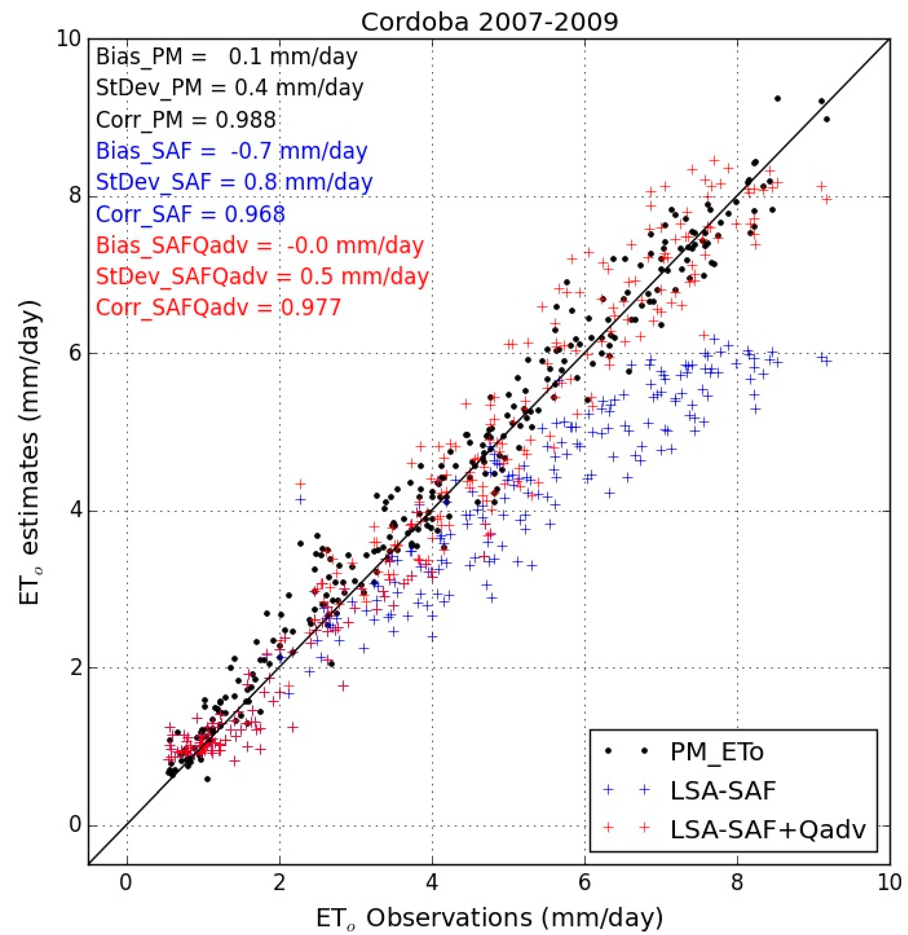
A similar plot is shown for Cordoba in Figure 2, now showing the LSA SAF estimates without considering LAE (as in the case above), as well as an adjusted value to take into account LAE (as in Equation (3)). The mean difference between LSA-SAF estimates and in situ observations is reduced from −0.7 mm/day to 0.1 mm/day, when the correction for LAE is introduced, while the standard deviation of differences also decreases from 0.8 mm/day to 0.5 mm/day.
These results were first published in [5]. A discussion of these results and implications for the practical use of the LSA SAF ETo product and Equation (3) are presented in the next section.
4. Discussion
The main purpose of this work is to draw the attention of water managers and irrigation advisors to the LSA SAF operational ETo product (being METREF its official acronym within the LSA-SAF) as an appropriate alternative for the FAO methodology. The physical basis of the two approaches are both sound, but they are derived along different routes. The LSA SAF product considers the T-ABL approach, based on thermodynamics of well-watered surfaces, whereas the FAO model is derived from a number of concepts postulated for the vegetation layer and the turbulent vertical transfer of water vapor in the atmosphere. T-ABL ETo implicitly includes entrainment processes at the top of the ABL, which are hidden in the empirical model constants in PM-ETo.
Because the thermodynamics-based T-ABL model does not account for local advection effects (LAE), it yields a correct estimate of ETo, which is consistent with this variable definition. As shown by [4,5] the T-ABL methodology can be easily extended to quantify LAE, by an additional energy term in (1). It is found that when the temperature is higher than 15 °C, this extra energy term is proportional to (Ta-15) in the Cordoba site, and that at the peak of the dry season it accounts for an extra 30% of ETo (see largest differences between blue and red lines in Figure 2).
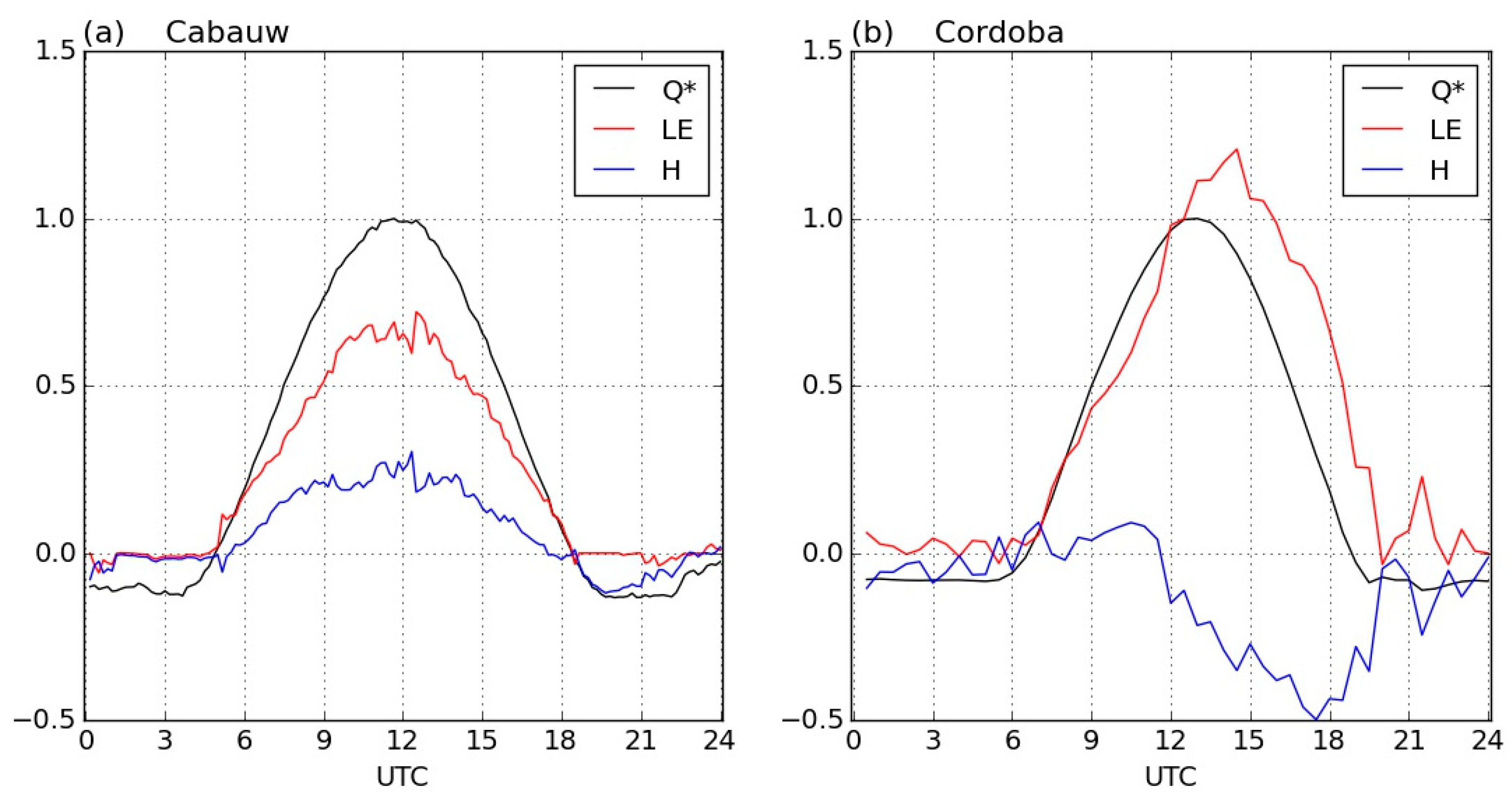
To illustrate the impact of LAE, the analyses by [5] show that at high temperatures the difference between Equations (1) and (3) can be as large as 30%. In order to discuss the LAE issue in more detail, Figure 3 shows the diurnal cycle of the main components of the surface energy balance, namely net radiation (Q*), sensible (H) and latent heat flux (L.ET). All of these were measured in a typical clear sky day in Cabauw (no LAE) and in Cordoba (with LAE). It is seen that during daytime L.ET is lower than Q* in Cabauw, whereas, in the Cordoba case, L.ET becomes greater than Q* after about 12 UTC (close to local noon) and then H becomes negative during the local afternoon. Although not shown, the additional energy that enhances L.ET, via the process described by the term Qadv in Equation (3), leads to evaporative cooling of the surface, which eventually drops below air temperature. A stable layer is then formed during daytime, consistent with the negative H values observed in Figure 3b.
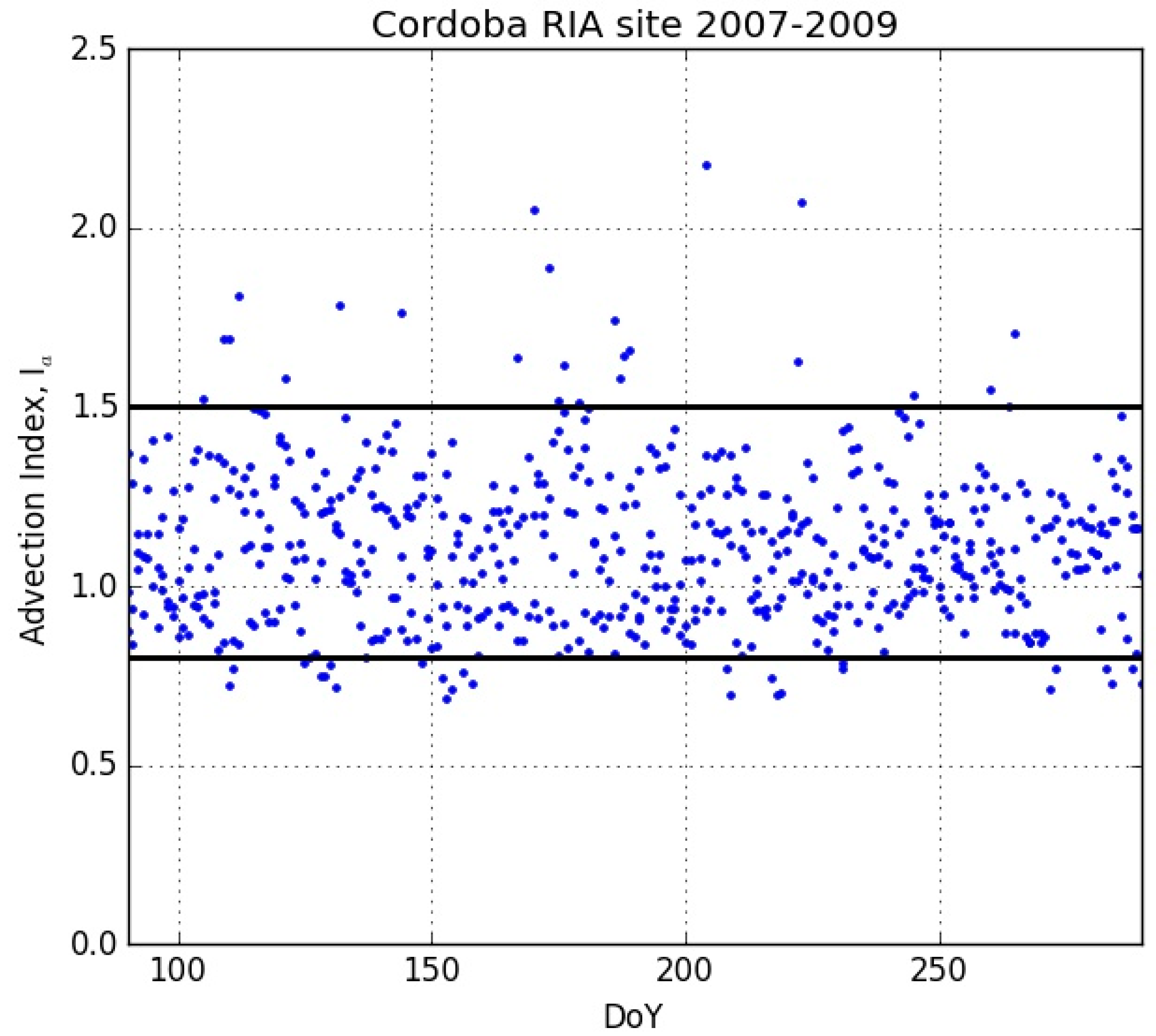
Confining ourselves to daily values in the growing season, i.e., between about April and September, 0.8Q* can be considered a suitable indicator for the occurrence of LAE, i.e., in cases where LAE is absent, daily L.ET will not differ much from 0.8Q*, whereas for the LAE case, L.ET will most likely exceed 0.8Q*. This value of L.ET being roughly 80% of net radiation was found for the Cabauw data, during the growing season. Using Equation (2) to determine Q*, a simple diagnostic tool is obtained to determine whether or not measured or calculated L.ET are affected by LAE, as also shown by [16]. To illustrate this, Figure 4 presents the so-called advection index, defined as Ia = L.ET/Q* (both L.ET and Q* correspond to daily averages), for the Cordoba site. Ia is plotted for a period encompassing the growing season, revealing that, for most of it, the measured L.ET is greater than 0.8Q* (for days-of-year between 147 and 300 shown in Figure 4, L.ET is always above this threshold), with Ia reaching values up to 1.5. This supports the notion that the Cordoba site is clearly affected by LAE, and particularly, as we move ahead of day-of-year 150 (i.e., from June onwards), L.ET becomes permanently higher than Q*, indicating an intensification of LAE.
It is noted that for Cabauw, the revised Makkink formula, where L.ET over the reference surface is proportional to solar radiation (), yields estimates very close to local observations [4,23,24]. On the other hand, a closer inspection of the literature revealed that for the Cordoba site, as is the case with LAE, the Hargreaves formula () dealt with in [1,25] also provides similar results to Equation (3) with the LAE adjustment (shown in Figure 2 for Cordoba). Both the Makkink and Hargreaves formulations are easier to use and can be applied as alternatives to PM-ETo in the LAE-free case and in the case LAE is meant to be accounted for, respectively.
The advection index can also be used to reveal effects of surface aridity. These refer to the impact on the estimation of ETo with the FAO-method, but when the input data are not gathered over reference grass. Because the surface atmospheric layer is itself affected by the radiation budget and its portioning between sensible and latent heat fluxes, measurements of temperature and humidity variables will necessarily be affected by the underling surface. As such, the input data should be adjusted in those cases, a practice that is often omitted. To illustrate the impact of this, we analyzed ETo estimated using data from the RIA Cordoba station [17] that is located close to the Cordoba lysimeter site, for which the Slob-deBruin estimate for Q* was tested by [5]. All input data for the FAO method were then obtained from in situ observations, but over non-irrigated ground.
Figure 5 shows the advection index Ia plotted for spring and early summer days, but now given by the calculated PM-ETo not adjusted for surface aridity, over the estimated net radiation using Equation (2). It is seen that in this case, Ia deviates even more generally from the 0.8 threshold than the values found for well-watered nearby grass (Figure 4). Adopting the rule of thumb that the LAE estimate of ETo is about 0.8Q*, this example shows that a combination of LAE and surface aridity effects can lead to significantly higher values, up to 100% or more of Q*. The LSA SAF method is not affected by surface aridity. From a practical point of view this is an enormous advantage, which is added to the fact that the LSA SAF approach does not need ground based-stations. The latter aspect is also relevant, when new underground water aquifers are explored, such as those present under the Sahara, or in locations where accurate weather data are simply absent.
It is clear from this example that PM-ETo values calculated with input data gathered over non-reference surfaces should be corrected for surface aridity. We note that in the literature there is no consensus about correction procedures. For this we refer to [12] and Annex 6 in [1] for example. It is outside the scope of this paper to discuss this topic. However, because errors in ETo due to surface aridity effects combined with LAE can be as high as 100% it is a very important aspect for users of PM-ETo. Note that our methodology does not suffer from these errors.
The LSA SAF ETo product does not account for LAE as required per definition [1,2], nor is it affected by aridity effects, and therefore can be used for irrigation advisory. Nevertheless, if one is interested in the actual ET of well-watered grass affected by LAE, then an adjustment is required for the LSA SAF values. As referred to above for the Cordoba lysimeter site and previously found by the authors for other similar sites, such correction may be parameterized as an additional term (Qadv), which is a linear function of near surface air temperature, i.e., with a term f(Ta), as shown in Equation (3), given by:
where the parameter To corresponds to the temperature above which the site systematically experiences LAE. Both regression coefficients, m and To, may vary with location and must be locally tuned using either local observations as described above for the lysimeter Cordoba site, or considering PM-ETo and LSA-SAF ETo as approximations of ET with and without LAE, respectively. A threshold of 0.8 may also be considered for the advection index to determine conditions with LAE. The index may be estimated using lysimeter ET observations (or PM-ETo estimates) and Slob-deBruin Q*. The latter is also distributed by the LSA SAF, as an auxiliary dataset within its METREF product.
5. Concluding Remarks
This research note concerns some aspects that may concern applications of the recently published LSA SAF product for ETo (METREF in the LSA SAF catalogue). Using observations from two very different sites and for situations where local advection effects (LAE) can be ignored and where they play a significant role, we showed that the LSA SAF provides ETo estimates that are basically LAE-free, thus fully consistent with the definition of ETo given in [1] and fulfilling the requirements specified in [2], as referred to above. The FAO PM methodology requires input data collected over a reference-like surface, otherwise estimated values may far exceed measured ones due to the so-called aridity effect; these do not affect the LSA SAF estimates based on the T-ABL approach.
There are other issues that should be considered in the practical application of T-ABL or FAO methods. For example, we ignored elevation effects on air temperature data, particularly when these were obtained from a numerical weather prediction model. The LSA SAF makes use of ECMWF global fields, which have a spatial resolution ranging from about 9 km (current operational model) to 75 km (ERA-Interim reanalyses [22]). Near surface (2 m) air temperature is then interpolated to each MSG/SEVIRI pixel, taking into account height differences and performing an orography adjustment [23]. Nevertheless, air pressure may also affect both T-ABL-ETo and PM_ETo, as it is hidden in the psychrometric constant γ, as discussed in [1] and [23]. We invite water managers and researchers involved in irrigation advisory to apply the LSA SAF ETo (METREF) product, pinpointing caveats and a way forward. Through interaction with the LSA SAF consortium the operational applicability of LSA SAF products can be improved.
Author Contributions
The authors contributed to the article as follows: Conceptualization, H.A.R.d.B. and I.F.T.; Methodology, H.A.R.d.B. and I.F.T.; Software, I.F.T.; Writing, H.A.R.d.B. and I.F.T.; Visualization, I.F.T.
Funding
This research received no external funding.
Acknowledgements
We thank Fred Bosveld (KNMI) and Pedro Gavilàn (IFAPA) for providing the Cabauw and Cordoba data. Satellite reference evapotranspiration and solar radiation products are made available by the EUMETSAT Satellite Applications Facility on Land Surface Analysis (LSA SAF; http://lsa-saf.eumetsat.int).
Conflicts of Interest
The authors declare no conflict of interest.
Annex—Terminology
| Name/Symbol | Meaning |
| ETo | Reference crop as defined in [1] and [2]; local advection effects are excluded. |
| ETc | Crop water requirement as defined in [1], and obtained via kc.ETo, with kc being a crop factor. Note that [1] introduced ETo and ETc to avoid the use of potential evapotranspriation, since the latter was generally used in as a maximum ET, without specifying the crop of surface. |
| PM-ETo | Version of the Penman-Monteith equation for estimating ETo, introduced by [1]. |
| LSA SAF ETo | Estimated using Equation (1) derived from thermodynamics and PBL-physics in [4] and validated in [5]. |
| METREF | The LSA SAF ETo estimates, as specified in the LSA SAF catalogue. |
| T-ABL | The model to estimate ETo derived from thermodynamics and atmospheric boundary layer (ABL) physics, leading to Equation (1). |
| Q* | Net radiation, i.e., the sum of the down-welling short and long wave radiation reaching the surface minus reflected (short and long wave) and the emitted (long wave) radiation. |
| Rs | Global radiation, or down-welling short wave radiation reaching the surface |
| Rext | Incoming shortwave radiation at the top of the atmosphere, often denoted as the extra-terrestrial radiation. |
References
- Allen, R.G.; Pereira, L.A.; Raes, D.; Smith, M. Crop Evapotranspiration—Guidelines for Computing Crop Water Requirements; FAO Irrigation and Drainage Paper 56; FAO: Rome, Italy, 1998; p. 293. [Google Scholar]
- Pereira, L.S.; Perrier, A.; Allen, R.G.; Alves, I. Evapotranspiration: Concepts and future trends. J. Irrig. Drain. 1999, 125, 45–51. [Google Scholar] [CrossRef]
- Allen, R.G.; Pruitt, W.O.; Wright, J.L.; Howell, T.A.; Ventura, F.; Snyder, R.; Itenfisu, D.; Steduto, P.; Berengena, J.; Baselga, J.; et al. A recommendation on standardized surface resistance for hourly calculation of reference ETo by the FAO56 Penman-Monteith method. Agric. Water Manag. 2006, 81, 1–22. [Google Scholar] [CrossRef]
- De Bruin, H.A.R.; Trigo, I.F.; Bosveld, F.C.; Meirink, J.F. A thermodynamically based model for actual evapotranspiration of an extensive grass field close to FAO reference suitable for remote sensing application. J. Hydrometeor. 2016, 17, 1373–1382. [Google Scholar] [CrossRef]
- Trigo, I.F.; de Bruin, H.; Beyrich, F.; Bosveld, F.C.; Gavilán, P.; Groh, J.; López-Urrea, R. Validation of reference evapotranspiration from Meteosat Second Generation (MSG) observations. Agric. For. Meteorol. 2018, 259, 271–285. [Google Scholar] [CrossRef]
- Schmidt, W. Strahlung und Verdunstung an freienWasserflächen; ein Beitrag zum Wärmehaushalt des Weltmeers und zum Wasserhaushalt der Erde (Radiation and evaporation over open water surfaces; a contribution to the heat budget of the world ocean and to the water budget of the Earth). Ann. Calender Hydrogr. Marit. Meteorol. 1915, 43, 111–124. [Google Scholar]
- Slatyer, R.O.; McIlroy, I.C. Evaporation and the principles of its measurement. In Practical Micrometeorology; CSIRO (Australia); UNESCO: Paris, France, 1961. [Google Scholar]
- De Bruin, H.A.R. A model for the Priestley-Taylor parameter. J. Appl. Meteorol. 1983, 22, 572–578. [Google Scholar] [CrossRef]
- Monteith, J.L. Accommodation between transpiring vegetation and the convective boundary layer. J. Hydrol. 1995, 166, 251–263. [Google Scholar] [CrossRef]
- McNaughton, K.G.; Spriggs, T.W. A mixed-layer model for regional evaporation. Bound.-Layer Meteorol. 1986, 34, 243–262. [Google Scholar] [CrossRef]
- McNaughton, K.G.; Jarvis, P.G. Predicting effects of vegetation changes on transpiration and evaporation. In Water Deficits and Plant Growth; Kozlowski, T.T., Ed.; Academic Press: New York, NY, USA, 1983; Volume 7, pp. 1–47. [Google Scholar]
- Temesgen, B.; Allen, R.G.; Jensen, D.T. Adjusting temperature parameters to reflect well-watered conditions. J. Irrig. Drain. Eng. 1999, 125, 26–33. [Google Scholar] [CrossRef]
- Geiger, B.; Meurey, C.; Lajas, D.; Franchistéguy, L.; Carrer, D.; Roujean, J.L. Near real-time provision of downwelling shortwave radiation estimates derived from satellite observations. Meteorol. Appl. 2008, 15, 411–420. [Google Scholar] [CrossRef] [Green Version]
- Greuell, W.; Meirink, J.F.; Wang, P. Retrieval and validationof global, direct, and diffuse irradiance derived from SEVIRI satellite observations. J. Geophys. Res. Atmos. 2013, 118, 2340–2361. [Google Scholar] [CrossRef]
- Monna, W.; Bosveld, F. In Higher Spheres: 40 Years of Observations at the Cabauw Site. 2013, p. 56. Available online: http://publicaties.minienm.nl/documenten/in-higher-spheres-40-years-of-observations-at-the-cabauw-site (accessed on 21 February 2019).
- Berengena, J.; Gavilán, P. Reference Evapotranspiration Estimation in a Highly Advective Semiarid Environment. J. Irrig. Drain. Eng. 2005, 131, 147–163. [Google Scholar] [CrossRef]
- Cruz-Blanco, M.; Gavilán, P.; Santos, C.; Lorite, I.J. Assessment of reference evapotranspiration using remote sensing and forecasting tools under semi-arid conditions. Int. J. Appl. Earth Obs. Geoinf. 2014, 33, 280–289. [Google Scholar] [CrossRef]
- Castellvi, F.; Gavilan, P.; Gonzalez-Dugo, M.P. Combining the bulk transfer formulation and surface renewal analysis for estimating the sensible heat flux without involving the parameter kB−1. Water Resour. Res. 2014, 50, 8179–8190. [Google Scholar] [CrossRef]
- De Bruin, H.A.R.; Holtslag, A.A.M. A simple parameterization of the surface fluxes of sensible and latent heat during daytime compared with the Penman-Monteith concept. J. Appl. Meteorol. 1982, 21, 1610–1621. [Google Scholar] [CrossRef]
- De Bruin, H.A.R. From Penman to Makkink. In Proceedings and Information: TNO Committee on Hydrological Research N°39, Den Haag, The Netherlands, 25 March 1987; Hooghart, J.C., Ed.; The Netherlands Organization for Applied Scientific Research TNO: Den Haag, The Netherlands, 1987; pp. 5–31. [Google Scholar]
- Pinker, R.T.; Tarpley, J.D.; Laszlo, I.; Mitchell, K.E.; Houser, P.R.; Wood, E.F.; Schaake, J.C.; Robock, A.; Lohmann, D.; Cosgrove, B.A.; et al. Surface radiation budgets in support of the GEWEX Continental-Scale International Project (GCIP) and the GEWEX Americas Prediction Project (GAPP), including the North American Land Data Assimilation System (NLDAS) project. J. Geophys. Res. 2003, 108, 8844. [Google Scholar] [CrossRef]
- Dee, D.P.; Simmons, A.J.; Berrisford, P.; Poli, P.; Kobayashi, S.; Andrae, U.; Balmaseda, M.A.; Balsamo, G.; Bauer, P.; Bechtold, P.; et al. The ERA-Interim reanalysis: configuration and performance of the data assimilation system. Q. J. R. Meteorol. Soc. 2011, 137, 553–597. [Google Scholar] [CrossRef] [Green Version]
- De Bruin, H.A.R.; Trigo, I.F.; Gavilán, P.; Martínez-Cob, A.; González-Dugo, M.P. Reference crop evapotranspiration estimated from geostationary satellite imagery. In Proceedings of the Remote Sensing and Hydrology, Jackson Hole, WY, USA, 27–30 September 2010; pp. 111–114. [Google Scholar]
- Makkink, G.F. Testing the Penman formula by means of lysimeters. J. Inst. Water Eng. 1957, 11, 277–288. [Google Scholar]
- Hargreaves, G.H.; Samani, Z. A Reference crop evapotranspiration from temperature. Appl. Eng. Agric. 1985, 1, 96–99. [Google Scholar] [CrossRef]
Figure 1.
Daily estimates of reference evapotranspiration as obtained by the LSA-SAF (blue crosses) versus daily in situ observations obtained for Cabauw (from eddy-covariance flux measurements) for the 2007–2012 period. For reference, Penman-Monteith (PM_ETo) estimates obtained using in situ observations are also plotted (black dots). The mean difference (bias), standard deviation of differences and correlation between estimations and observed time-series are also shown.

Figure 2.
Daily estimates of reference evapotranspiration as obtained by the LSA-SAF without (blue crosses) and with an adjustment term to account for local advection effects (red crosses), versus daily in situ observations obtained for Cordoba Lysimeter site, for the 2007–2009 period. For reference, Penman-Monteith (PM_ETo) estimates obtained using in situ observations at the lysimeter site are also plotted (black dots). The mean difference (bias), standard deviation of differences and correlation between estimations and observed time-series are also shown.

Figure 3.
Diurnal variation of the terms of the energy budget equation—latent (red line) and sensible (blue line) heat fluxes and net radiation (black line)—on a sunny day for (a) Cabauw (28 May 2012, no local advection) and (b) the lysimeter Cordoba site (29 July 2009, with local advection). All values are based on observations gathered at both sites and are normalized by the local net radiation maximum.

Figure 4.
Advection-index being the ratio of daily means of actual L.ET and Q*, as a function of day of year (DoY). Ia is estimated as the ratio between daily net radiation (obtained via Equation (2)) and daily latent heat flux obtained from observations taken over the well-watered Cordoba site (see also Figure 1 in [16]). The lower line represents the 0.8Q* threshold beyond which LAE should be taken into account.

Figure 5.
As in Figure 4, but Ia is estimated using observations gathered in the RIA station close to Cordoba (in situ observations gathered over non-irrigated surface).
Figure 5.
As in Figure 4, but Ia is estimated using observations gathered in the RIA station close to Cordoba (in situ observations gathered over non-irrigated surface).

© 2019 by the authors. Licensee MDPI, Basel, Switzerland. This article is an open access article distributed under the terms and conditions of the Creative Commons Attribution (CC BY) license (http://creativecommons.org/licenses/by/4.0/).
Share and Cite
MDPI and ACS Style
de Bruin, H.A.R.; Trigo, I.F. A New Method to Estimate Reference Crop Evapotranspiration from Geostationary Satellite Imagery: Practical Considerations. Water 2019, 11, 382. https://doi.org/10.3390/w11020382
AMA Style
de Bruin HAR, Trigo IF. A New Method to Estimate Reference Crop Evapotranspiration from Geostationary Satellite Imagery: Practical Considerations. Water. 2019; 11(2):382. https://doi.org/10.3390/w11020382
Chicago/Turabian Stylede Bruin, Henk A. R., and Isabel F. Trigo. 2019. "A New Method to Estimate Reference Crop Evapotranspiration from Geostationary Satellite Imagery: Practical Considerations" Water 11, no. 2: 382. https://doi.org/10.3390/w11020382
Note that from the first issue of 2016, this journal uses article numbers instead of page numbers. See further details here.