Statistical and Numerical Assessments of Groundwater Resource Subject to Excessive Pumping: Case Study in Southwest Taiwan

Abstract

Groundwater, a salient water resource in Taiwan, has been subject to incessant and excessive pumping, inducing serious regional land subsidence and seawater intrusion. This study aims at assessing how excessive pumping impacts groundwater variations over the Pingtung Alluvial Plain (PAP) in Southwest Taiwan using both statistical and numerical techniques. We apply nonparametric methods to analyze the changing point and annual trend in various hydro-meteorological time series (e.g., rainfall, temperature, and groundwater levels (GLs)). Afterwards, we employ an integrated surface-subsurface model referred to as WASH123D to simulate GLs under the pumping-free scenario; any discrepancies identified between simulated and observed GLs could be an indicator of unregulated/illegal pumping. We find that annual GLs exhibit a significant increasing (decreasing) trend in the western (eastern) PAP. Our numerical experiment reveals diverging trends in simulated and observed GLs, mostly at the downstream of all the major tributaries, suggesting the consequence of unregulated/illegal pumping. Furthermore, upstream pumping may reduce lateral flow towards the downstream coastal area, triggering land subsidence in remote locations.

1. Introduction

Regulating water use in dry seasons is always challenging for less available surface water supply, thereby stimulating the development and withdrawal of groundwater resources [1,2]. As a result, groundwater can be depleted under the scenario of reckless, excessive pumping. Overuse of groundwater can induce paramount environmental issues, including modification of baseflow, land subsidence, and seawater intrusion [3,4,5,6,7]. To ensure sustainable groundwater resource, effective groundwater resource management able to take into account the interactions between surface and subsurface water at varied spatio-temporal scales is needed. One means to constitute pertinent management policies (e.g., groundwater divisions and availability, legal pumping amounts, control measures, and decision making) is through the application of a physically-based groundwater model [8].

The utility of combining statistical with numerical assessments can be seen in several respects. An example of our particular interest is to facilitate the understanding of the causal relationship between the variations in groundwater levels (GLs) and land subsidence. Supposedly, a dropping GL due to excessive pumping is a prior event to land subsidence. The rationale behind this is the acceleration of the consolidation-drainage process in the mud layer, induced by a more rapid reduction in the pore pressure of the sand/gravel layer (of high hydraulic conductivity) than that of the mud layer due to excessive pumping [9,10]. Statistical analyses such as trend and change-point analyses [11,12,13,14] thus can identify GLs of significant decreasing trends and the shift in the mean to indicate areas of further land subsidence. However, without knowing the pumping locations and history, numerical simulations of flexible model configurations seem to be the one and only way to establish a link between the drops in GLs with unregulated/illegal pumping. As an alternative to a plausible interpretation of the model results, descriptive information regarding hydro-meteorological variables derived from statistical analysis is of great importance, especially in a region with known or suspicious pumping activity.

Groundwater source identification belongs to a specific track of the inverse problems that can be seen through many experimental studies using various simulation and optimization methods [15,16]. Nonetheless, most of the experiments dealt with a limited number of wells, thereby showing little success for real cases. Our research purpose is to substantiate the unregulated/illegal pumping, rather than pinning down unknown groundwater well locations and pumping rates. More specifically, we wish to achieve two objectives: (1) to apply a suite of statistical techniques to examine various groundwater-related hydro-meteorological variables and (2) to conduct numerical simulations for GLs under the pumping-free scenario in the same region, reverse engineered to disclose the impact of unregulated/illegal pumping. The rest of this paper is organized as follows. Section 2 describes the study area and hydro-meteorological data used in this study. Section 3 introduces various statistical methods and the numerical model and its configuration. Section 4 presents results from both statistical and numerical assessments in the context of discussing the impact of unregulated/illegal pumping on groundwater variations. Section 5 lists some important takeaways.

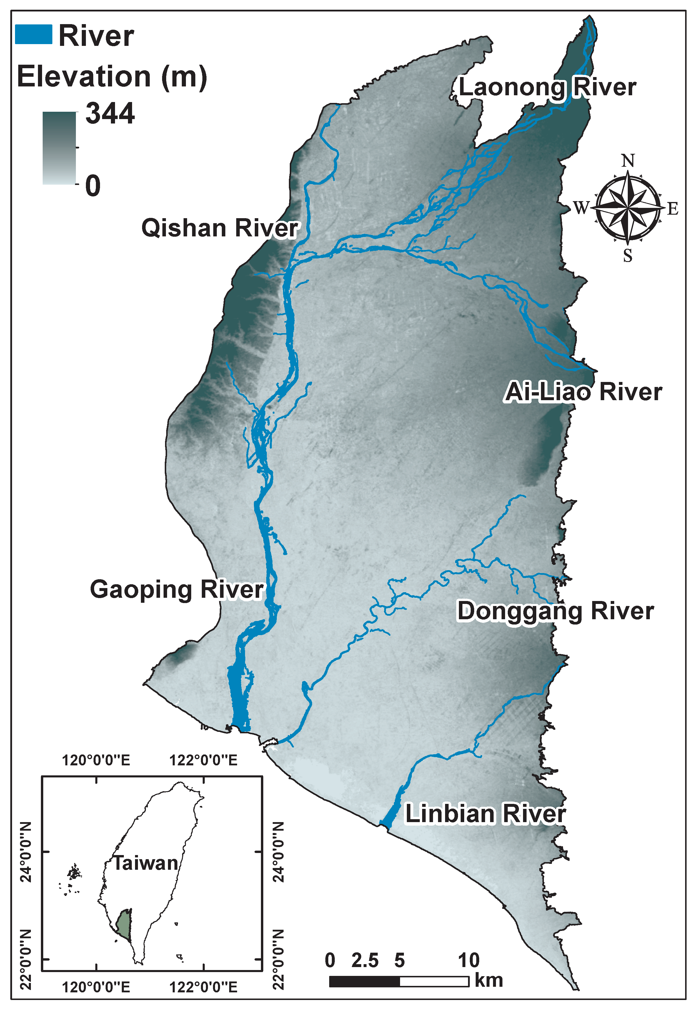
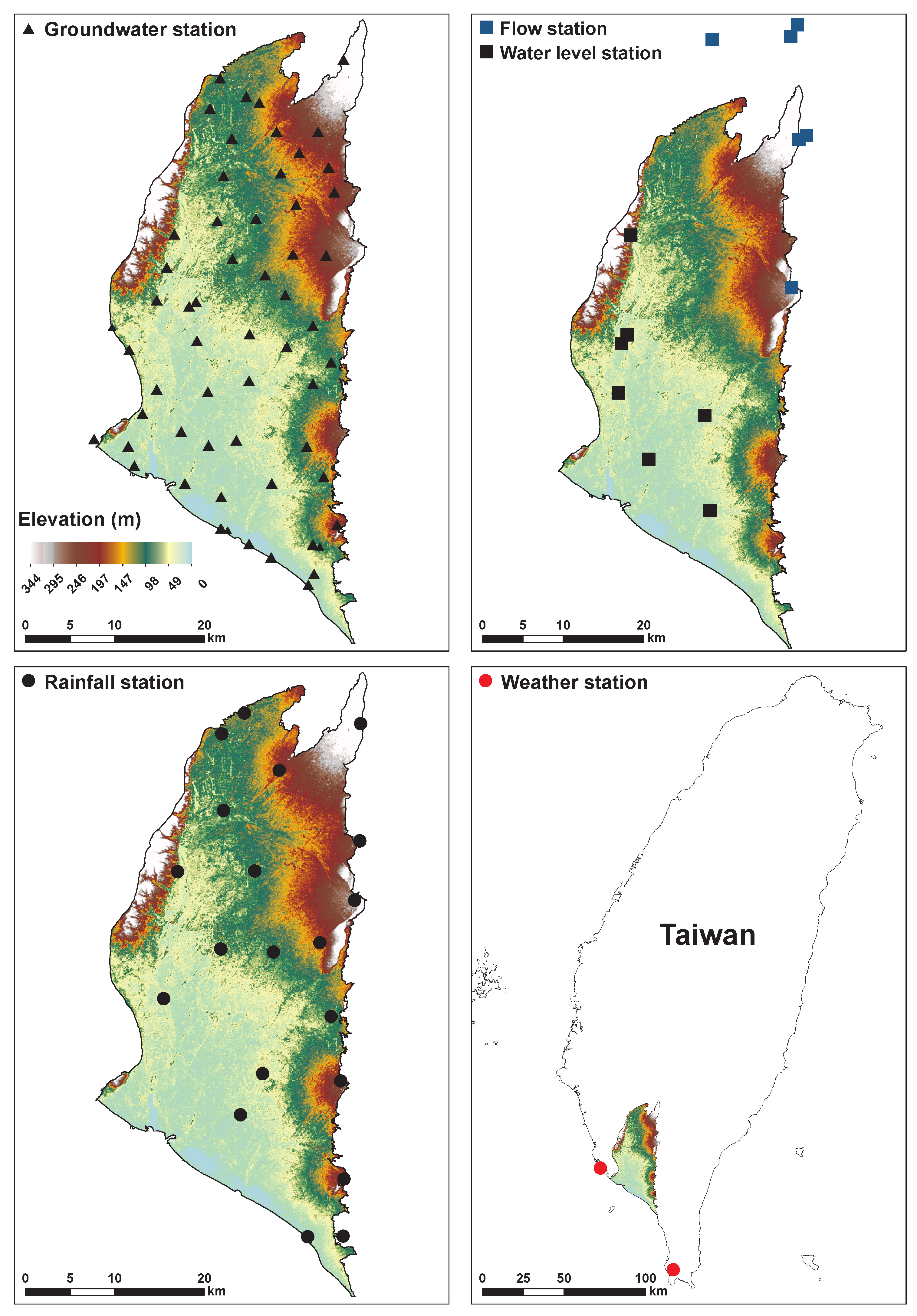
2. Study Area and Data

In Southwest Taiwan, the Pingtung Alluvial Plain (PAP, Figure 1) is characterized by excessive pumping and serious land subsidence. The PAP has an area of 1232 km${}^2$ and a gradually-varying topography from the apex over the northeastern portion to the tail over the south-southwestern coastal area. Most of the PAP area is designated as flatlands of low elevation (<100 m). Immediately next to the eastern boundary of the Central Mountain Range are three major groundwater recharge zones, namely the Laonong, Ai-Liao, and Linbian alluvial fans. There is no official, joint surface and subsurface water regulation and management in place, and the groundwater problem is unique in the PAP. According to the earlier survey conducted by the Council of Agriculture, approximately 90% of wells were either unregistered or illegal (≈15,000 of 17,000) in the PAP [17], and that number is growing. Therefore, it is impossible to monitor or estimate accurately the amount of groundwater abstraction over the years, as seen by many preceding projects funded by the Water Resources Agency (WRA).

This study uses various hydro-meteorological data, including river discharge, surface and GLs, rainfall, and temperature. Whereas the hydrological and hydrogeological data were mainly obtained from the WRA, the meteorological data were from the Central Weather Bureau (CWB) of Taiwan. Specifically, we have river flow and water level data from six and seven WRA-owned hydrological stations along the main streams of the PAP, respectively. Over the PAP, we have a total of 66 WRA-owned monitoring wells, in which a total of 151 gauges for GLs at different vertical layers are installed. Preliminary quality assurance and checks have been performed to eliminate those gauges showing limited data records (e.g., less than 10 years), too many data gaps, or erratic data fluctuations, resulting in a remaining 127 gauges with GL data ranging from 1994–2014. Regarding meteorological data, we acquired precipitation and temperature data from 20 rain gauges and two weather stations from the CWB, respectively. The period of records for the meteorological data is equal to or longer than that for the groundwater data. Figure 2 displays the spatial distribution of the various stations mentioned above; note that the two selected weather stations (i.e., Hengchun and Kaohsiung) are situated outside, but in the vicinity of the PAP because no other stations with long-term temperature records are available inside the PAP.

3. Methodology

The two assessment methods are described in this section. Firstly, regarding the statistical assessment, trend and change-point analyses are introduced. Secondly, regarding the numerical assessment, a groundwater model and its configurations are described, including the determination of model parameters (e.g., hydraulic conductivity), 3D mesh, and boundary conditions.

3.1. Statistical Assessment

3.1.1. Trend Analysis

The first statistical analysis conducted was to examine whether a data series exhibited a significant trend in time. Such analysis can be achieved by applying the Mann–Kendall test [18,19] to the data series, say $\{x_1,x_2,\dots ,x_n\}$. The M-K test is one particular hypothesis test, loosely speaking, that specifies the null and alternative hypotheses (i.e., $H_0$ and $H_1$) as the data series showing insignificant and significant trends, respectively. The test statistic for the M-K test is the standard normal variate, Z, which is determined by variable K through:

$$Z=\left\{\begin{array}{c}\hfill \frac{K-1}{\sqrt{var\left(K\right)}}\mathrm{for}K>0,\\ \hfill 0\mathrm{for}K=0,\\ \hfill \frac{K+1}{\sqrt{var\left(K\right)}}\mathrm{for}K<0,\end{array}\right.$$

(1)

where $var\left(K\right)=\frac{n(n-1)(2n+5)}{18}$ and n is the data size ($\ge 2$). K can be calculated from:

$$K=\sum _{i=1}^{n-1}\sum _{j=i+1}^{n}sgn(x_j-x_i),\mathrm{where}\left\{\begin{array}{c}sgn(x_j-x_i)=+1,\mathrm{for}{x}_j>x_i,\hfill \\ sgn(x_j-x_i)=0,\mathrm{for}{x}_j=x_i,\hfill \\ sgn(x_j-x_i)=-1,\mathrm{for}{x}_j<x_i.\hfill \end{array}\right.$$

(2)

To state that a data series exhibits a significant trend, the test statistic $\left|Z\right|$ has to be greater than a critical value; that is, rejecting $H_0$ for a two-tailed test. Typically, an $\alpha$ equal to 0.05 is adopted for deriving the critical value as 1.96.

To supplement the M-K test, which indicates only the significance of the trend, we adopt Sen’s slope [20] for estimating the average rate of change ($\beta$) in a data series. Sen’s slope is defined as the median of all the slope values derived from any two data points from the data series, or mathematically,

$$\beta =median\left(\frac{x_j-x_i}{j-i}\right),\mathrm{for}j>i.$$

(3)

Unlike the regression-based slope estimator, Sen’s slope is known to be less affected by data outliers.

3.1.2. Change-Point Analysis

To identify change points (i.e., shifts in the mean) in a data series, as the second part of our statistical assessment, we adopted the Mann–Whitney–Pettitt test [21]. The M-W-P test can also be interpreted as a particular hypothesis test that specifies $H_0$ and $H_1$ as the data series showing an insignificant and significant change point, respectively. To apply the M-W-P test, we first transformed the data series $\{x_1,x_2,\dots ,x_n\}$ into the U series, namely $\{u_1,u_2,\dots ,u_n\}$, expressed by:

$$u_t=\sum _{i=1}^t\sum _{j=1}^{n}sgn(x_i-x_j),\mathrm{where}\left\{\begin{array}{c}sgn(x_i-x_j)=+1,\mathrm{for}{x}_i>x_j,\hfill \\ sgn(x_i-x_j)=0,\mathrm{for}{x}_i=x_j,\hfill \\ sgn(x_i-x_j)=-1,\mathrm{for}{x}_i<x_j.\hfill \end{array}\right.$$

(4)

The maximum u is then determined as:

$$K_p=\underset{1\le t\le n}{max}\left|U\right|.$$

(5)

Lastly, $K_p$ is plugged into the following equation to calculate P,

$$P=1-exp\left(\frac{-6K_p^2}{n^2+n^3}\right).$$

(6)

In general, if $P>0.9$, the null hypothesis is rejected, indicating that a change point has been identified.

We also adopted another test referred to as the Kruskal–Wallis test [22] to attest to the change point identified by the M-W-P test. The K-W test, also called the one-way analysis of variance on ranks, is used to examine whether m independent samples originate from the same population. The null hypothesis of the K-W test is that the medians of all m samples are statistically indistinguishable; that is, if $H_0$ is rejected, then at least one group of the samples is different from the others. To accommodate the K-W test for our case as the supplement to the M-W-P test, we performed the following analysis. If the M-W-P test is able to divide the original data series into m groups (i.e., change pints identified), say $\{x_{11},x_{12},\dots ,x_{1n}\},\{x_{21},x_{22},\dots ,x_{2n}\},\dots ,\{x_{m1},x_{m2},\dots ,x_{mn}\}$, we will see if the null hypothesis of the K-W can also be rejected to confirm the result of the M-W-P test. The criterion for rejection of the K-W test is based on the inequality between the test statistic $K_w$ and ${\chi }_{\alpha ,\nu }^2$, where $\alpha =0.05$ is used and $\nu =m-1$ is the degree of freedom. $K_w$ is determined by the equation below:

$$K_w=\frac{12}{N(N-1)}\sum _{i=1}^m\frac{R_i^2}{n_i}-3(N+1),$$

(7)

where $N={\sum }_{i=1}^m{n}_i$ and $R_i$ denotes the sum of ranks on data group i,

$$R_i=\sum _{j=1}^{n_i}RANK\left(x_{ij}\right).$$

(8)

For instance, if $m=2$ (i.e., one change point identified), we will see if $K_w$ calculated from the above equations is greater than ${\chi }_{0.05,1}^2=3.84$ for the confirmation.

3.2. Numerical Assessment

3.2.1. Groundwater Model: WASH123D

Among a variety of groundwater models, WASH123D, an integrated multimedia, multi-process, physics-based computational model used for describing watershed-scale hydrology [23,24,25], was adopted in this study. Developed by [23], WASH123D covers dendritic 1D river/stream/canal networks, the 2D overland regime, and 3D subsurface media, including the vadose and saturated zones. The governing equation is derived based on the continuity of fluid and solid mass, the incompressibility of solids, and Darcy’s law. The simulation is conducted with finite-element approaches for computations at varied spatial-temporal scales. It is typical to use the cross-section-averaged 1D diffusive wave equation, the depth-averaged 2D diffusive wave equation, and the 3D Richards equation. The equations are solved with semi-Lagrangian and Galerkin finite-element methods to determine canal network flow, overland flow, and variably-saturated subsurface flow [26]. WASH123D has been applied to many regionally-significant projects and was chosen by the U.S. Army Corps as the core computational code for coast and watershed studies. A revamped version of the WASH123D model has also been applied to many flood mitigation and groundwater problems [27,28,29,30].

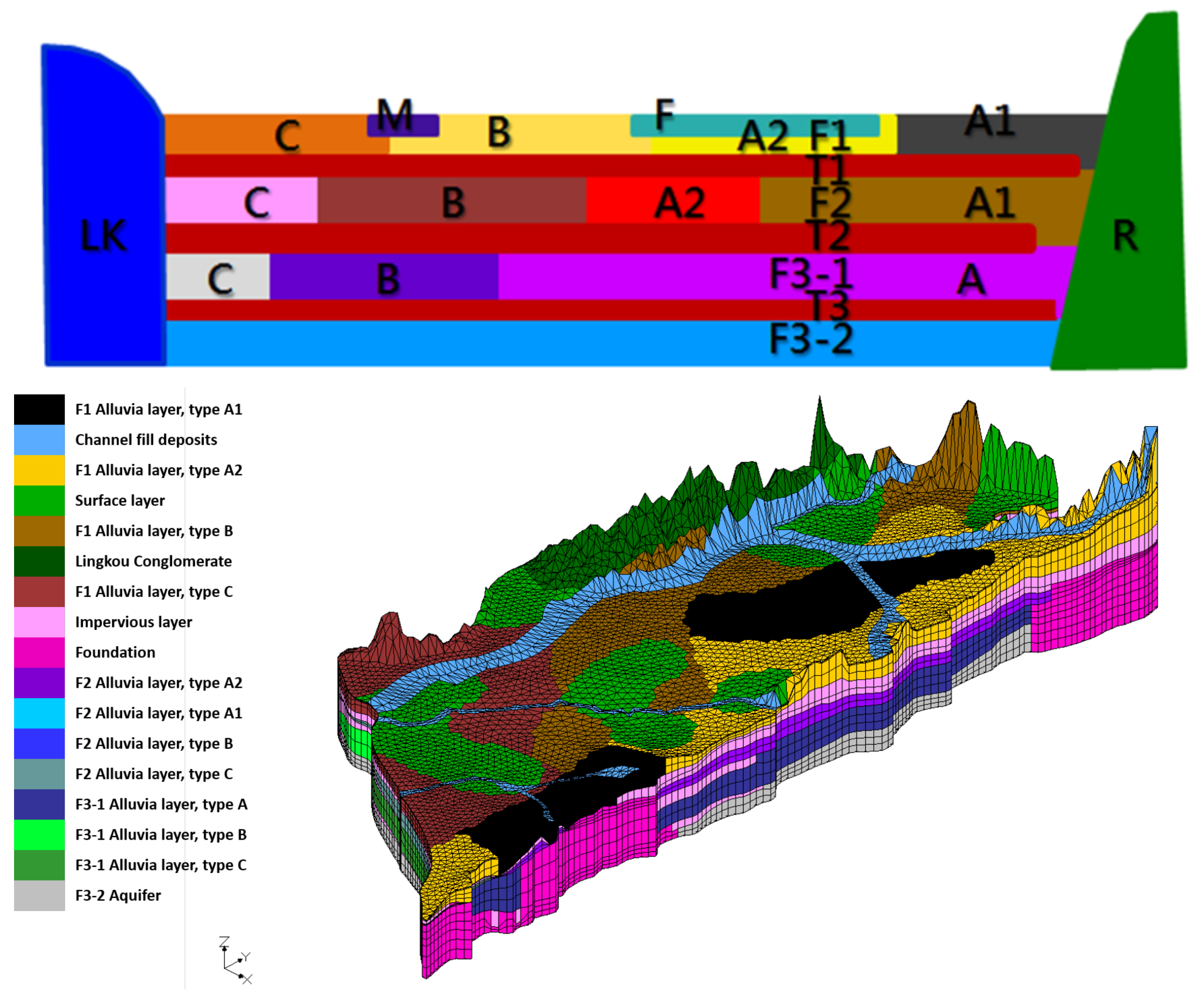
3.2.2. Hydrogeological Analysis

To initiate a numerical simulation, a priori parameters such as hydraulic conductivity values for the PAP were determined based on hydrogeological analysis. According to the core drilling report provided by the Central Geological Survey (CGS), there were seven vertical layers identified for the PAP: (from top to bottom) Aquifer 1 (F1), Aquitard 1 (T1), Aquifer 2 (F2), Aquitard 2 (T2), Aquifer 3-1 (F3-1), Aquitard 3 (T3), and Aquifer 3-2 (F3-2). In each aquifer (except for F3-1 with monotonous geological materials), Zones A, B, and C were further classified (e.g., F1/A, F1/B, and F1/C for Aquifer 1) with mostly gravels, coarse sands, and silts and clays, respectively. Previous pumping tests have shown that even in the same aquifer and zone, hydraulic conductivity values may vary. Thus, we divided F1/A and F2/A into F1/A1, F1/A2, F2/A1, and F2/A2. We delineated the thickness and span of each aquitard based on the drilling report and hydrogeological profiles. Again based on the drilling report and the locations of river channels, we delineated the surface mud layer (M) and fluvial deposit (F). Over the western and eastern boundaries of the PAP, we determined two independent units as Lingkou conglomerate (LK) and bedrock (R), respectively; the vertical profiles of the boundary units were assumed to be uniform.

Figure 3 illustrates all the hydrogeological units indicated above, and

Table 1. Hydrogeological units in the PAP and associated hydraulic conductivity (K) values used on this study.

Hydrogeological Unit		ID	Pumping Test Results			Lateral K
Name	Abbr.		No. Tests	Ave.K	Std. Log(K)
Mud Layer	M	13	-	-	-	$7\times {10}^{-8}$ m/s
Fluvial Deposit	F	14	-	-	-	$2\times {10}^{-5}$ m/s
Aquifer 1/A1	F1/A1	1	7	$2.12\times {10}^{-3}$ m/s	0.32	$2\times {10}^{-3}$ m/s
Aquifer 1/A2	F1/A2	2	8	$5.69\times {10}^{-4}$ m/s	0.33	$7\times {10}^{-4}$ m/s
Aquifer 1/B	F1/B	3	13	$3.31\times {10}^{-4}$ m/s	0.5	$4\times {10}^{-4}$ m/s
Aquifer 1/C	F1/C	4	13	$2.32\times {10}^{-4}$ m/s	0.75	$1.9\times {10}^{-4}$ m/s
Aquifer 2/A1	F2/A1	5	4	$9.84\times {10}^{-4}$ m/s	0.06	$1\times {10}^{-3}$ m/s
Aquifer 2/A2	F2/A2	6	18	$8.39\times {10}^{-4}$ m/s	0.44	$6\times {10}^{-4}$ m/s
Aquifer 2/B	F2/B	7	15	$2.69\times {10}^{-4}$ m/s	0.38	$3\times {10}^{-4}$ m/s
Aquifer 2/C	F2/C	8	4	$2.27\times {10}^{-4}$ m/s	0.23	$5\times {10}^{-5}$ m/s
Aquifer 3-1/A	F3-1/A	9	30	$1.91\times {10}^{-4}$ m/s	0.5	$5\times {10}^{-4}$ m/s
Aquifer 3-1/B	F3-1/B	10	12	$1.86\times {10}^{-4}$ m/s	0.59	$2\times {10}^{-4}$ m/s
Aquifer 3-1/C	F3-1/C	17	5	$4.31\times {10}^{-4}$ m/s	0.48	$4\times {10}^{-5}$ m/s
Aquifer 3-2	F3-2	11	16	$5.13\times {10}^{-4}$ m/s	0.55	$5\times {10}^{-4}$ m/s
Aquitards	T1–T3	15	-	-	-	$1\times {10}^{-8}$ m/s
Lingkou Cg †	LK	12	-	-	-	$2\times {10}^{-5}$ m/s
Bedrock	R	16	-	-	-	$1\times {10}^{-8}$ m/s

† conglomerate.

lists these units and associated hydraulic conductivity values based on the pumping tests conducted by the CGS. The soil retention curves for the unsaturated zone were generated using the power-law-related model and assumed that the saturated hydraulic conductivity of the 3D subsurface flow in the horizontal direction was 10-times that in the vertical direction [28,30]. Regarding the surface parameter, Manning’s coefficients (Mn) for the rivers was referenced to field investigations conducted by the WRA. The Mn’s for land are classified based on the land coverages and then determined by previous studies and fine-tuned results [27]. The surface parameters adopted are shown in

Table 2. Additional parameters used for WASH123D simulations in the PAP.

Channels (1D)	Land Surfaces (2D)
$\mathit{Mn}$	$\mathit{Mn}$
0.028–0.040	Agricultural (0.20)
	Forestry (0.30)
	Traffic (0.10)
	Water (0.05)
	Building (0.10)
	Other (0.15)

.

3.2.3. Mesh Generation

Mesh generation begins with the development of 1D river networks, followed by the generation of 2D triangular grids. We use the predefined hydrogeological units, land use data, and the digital terrain model for generating 2D grids and mapping various input data to the grid nodes. The generation of 3D grids depends on the information regarding the vertical layers of the hydrogeological units thus far mentioned.

According to the WRA cross-section survey, the locations of the major tributaries in the PAP (i.e., the Gaoping, Donggang, and Linbian Rivers) were delineated, and the total number of cross-sections for the 1D river networks was determined as 271 for our simulation. The deepest points of the riverbeds and the river widths can also be determined. In each river cross-section, data over the left, riverbed, and right banks were incorporated into the hydrogeological units for generating the 2D overland grids, resulting in 4859 nodes and 9350 grids for the 2D simulation. Regarding the 3D subsurface grids, the thickness was 1 m for near-surface grids and gradually enlarged downward, and each aquifer was further divided into three sub-layers. Thus, 72,885 nodes and 130,900 grids were generated for the 3D simulation, and the modeling depth was approximately 250 m (see Figure 3).

3.2.4. Boundary Conditions

Various types of boundary conditions, determined based on physical reasoning, are essential to supplement the governing equations of WASH123D. As previously mentioned, the WRA and CGS have conducted detailed hydrogeological surveys in this region, to which various groundwater models apart from the WASH123D have also been applied [31]. Model configurations including boundary conditions were thus determined in accordance with data and information acquired from these studies and previous reports [32,33,34]: The eastern boundary of the modeling domain was set over the foot of the eastern mountains, located at the areas along Qishan, Meinong, Taishan, Daxiang, and Fangshan. Because the eastern boundary adjoins the slightly metamorphic Miocene stratum, we adopted a no-flow boundary condition. The western and northern boundaries were set over the Fengshanhilly line and another Miocene stratum, respectively; to ensure the highest numerical stability, we also adopted no-flow boundary conditions. Over the south along the coast line, we used a constant-head boundary.

4. Results and Discussion

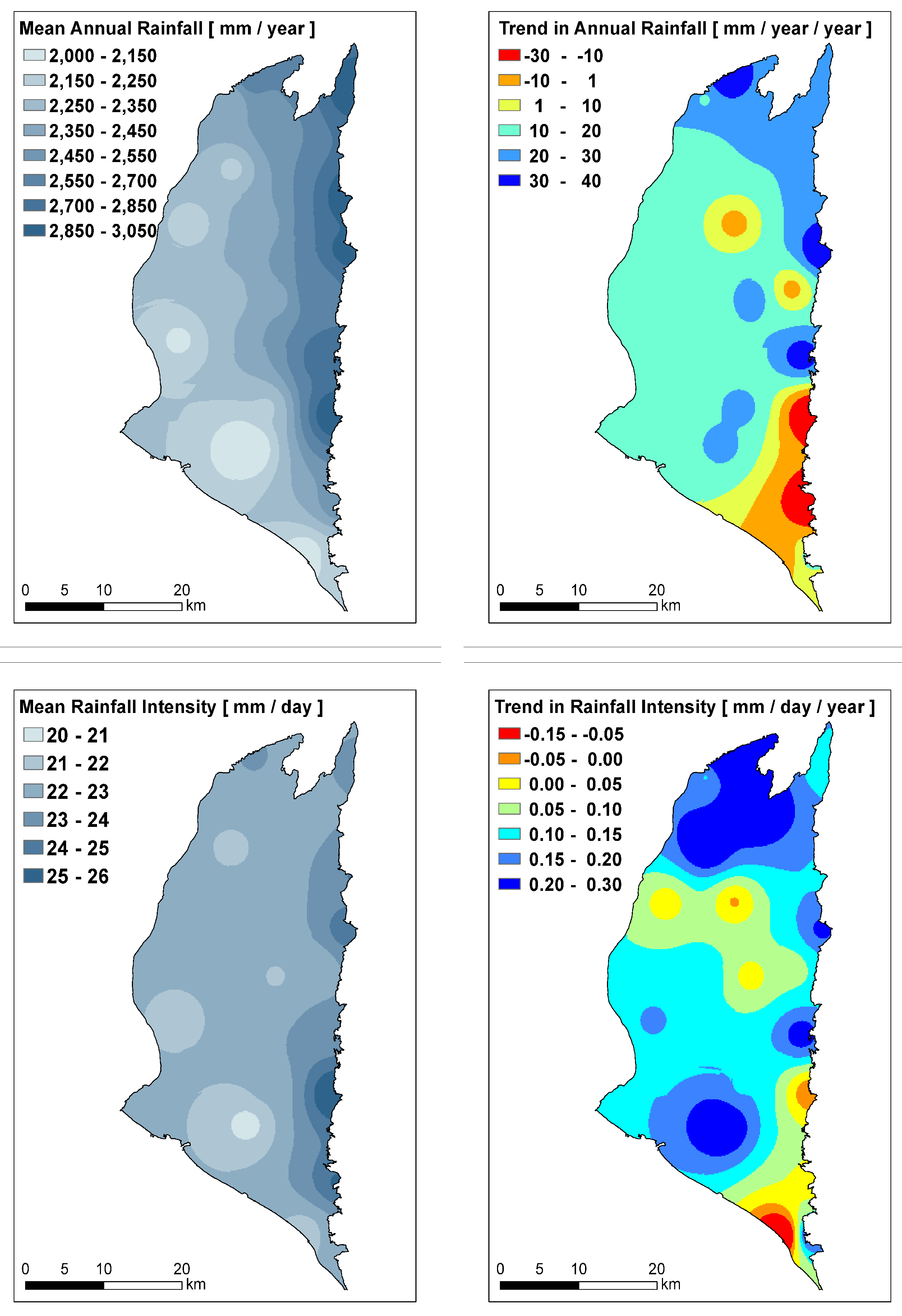
4.1. Interannual Variations in Hydro-Meteorological Conditions

Our statistical assessment begins with performing trend and change-point analyses of various hydro-meteorological variables at the annual scale. The first variable of interest was annual rainfall over the PAP. Figure 4 shows the mean annual rainfall amounts and intensity, associated with the results of trend analysis. Both the amounts and intensity peak at the eastern mountains and gradually decreased towards the flatlands and the coastal area. Many stations exhibited an increasing trend in both the amounts and intensity, while some stations showed the opposite over the southeastern area (e.g., Fangliao and Laiyi); however, neither trend was significant. Change-point analysis revealed only two stations, namely Chishan and Nanzhou, experiencing an abrupt change in rainfall intensity in the year 2004. Overall, annual rainfall in this area has been quite stationary over the past decades.

Unlike the annual rainfall amounts and intensity, annual mean temperatures at Hengchun and Kaohsiung stations exhibited a significant increasing trend. The rates of change at the two stations were calculated as 0.24 and 0.26 ${}^{\circ }$C per decade, both at a 5% significance level. Change-point analysis identified the year 1997 when both stations experienced an abrupt shift in the mean temperature, and we found that the rates of change were higher for the post-change point epoch. To explore the effect of increasing temperature on the losses of water in the study region, we plugged the temperature and other pertinent data into the Hamon equation [35] to calculate annual potential evapotranspiration (PET). The results suggested that mean annual PET over the PAP was approximately 1500 mm. The increasing trend in PET was basically inherited from the trend in temperature, and the rate of change was approximately 23 mm per decade. Detailed temperature records at the two weather stations from 1981–2014 are listed in

Table 3. Temperature records (${}^{\circ }$C) at Hengchun and Kaohsiung stations.

Year	Hengchun	Kaohsiung	Year	Hengchun	Kaohsiung
1981	25.21	25.00	1998	26.06	25.83
1982	24.82	24.83	1999	25.12	25.19
1983	24.90	24.76	2000	25.32	25.13
1984	24.54	24.33	2001	25.20	25.16
1985	24.72	24.22	2002	25.44	25.66
1986	24.21	24.43	2003	25.27	25.43
1987	25.30	25.16	2004	25.12	25.22
1988	25.16	24.87	2005	25.05	25.05
1989	24.77	24.95	2006	25.90	25.68
1990	25.12	25.13	2007	25.77	25.46
1991	25.14	25.34	2008	25.37	25.14
1992	24.95	24.88	2009	25.40	25.35
1993	25.20	25.11	2010	25.37	25.44
1994	25.37	25.21	2011	24.72	24.95
1995	24.95	24.65	2012	25.48	25.43
1996	24.97	24.83	2013	25.56	25.55
1997	24.97	24.98	2014	25.59	25.59

.

The follow-up, critical variable to be examined is annual GLs over the PAP. The mean GL at all the layers showed a gradual decrease from the apex to tail (Figure 5a–c; spatial results for Aquifer 3-2 are omitted due to the insufficient number of stations). The results of trend analysis, shown in Figure 5d–f, reveal that approximately 1/3rd of the 127 gauges exhibited an increasing trend over the recent decades, and these gauges were mostly located at the Gaoping River (from the western part to the tail of the PAP). Such an increasing trend is partly attributed to the natural geological property of this area (e.g., topography and Lingkou conglomerate as the western boundary), which manifests the flow accumulation in the long run if there is no witness to excessive pumping. The remaining 2/3 of the gauges, mostly located at the eastern part of the PAP (Linbian and Ailiao Rivers), exhibited a decreasing trend. At some of the stations (e.g., Wanfu, Daxiang, and Fangliao), the decreasing trend can be significant at multiple layers, suggesting that the local groundwater resource has been severely undermined. Change-point analysis identified a total of 91 gauges (∼70%) experiencing abrupt shifts in the GL, and the results are summarized in histograms for the many gauges at different layers in Figure 6. In general, the histograms for Aquifers 1 to 3-1 display a bimodal distribution: The two most frequent timings identified as the change points were around 2005 and 2008.

We further investigated the variations in GLs before and after the identified change points. For the pre-change point epoch, notable increasing trends can be observed over the Lingkou hill area (Figure 7a–c), consistent with the aforementioned area of the same trend. Moderate trends in either direction (<0.1 m/year) prevailed in other areas, but the only exception of a significant decreasing trend (<−0.3 m/year) took place at several stations in Aquifer 3-1. This neighborhood is referred to as Jiadong, Fangliao, and Linbian Townships, coinciding with the sensitive area identified and declared by the WRA as severe land subsidence (see the land subsidence map, Figure S1, in the Supplementary Materials). This finding is also in agreement with the causal relationship between the decreases in GLs and successive land subsidence [9,10]. For the post-change point epoch, the western increasing trend was no longer significant at the deeper layers. In contrast to the pre-change point pattern, vast eastern areas of significant decreasing trends stood out as the most pronounced pattern (Figure 7d–f). Based on the same concept of GLs versus land subsidence, we can postulate a possibility of continuing land subsidence in the sensitive area.

The above findings indicate that the stationary recharge (i.e., no significant trend in annual rainfall) seems to have difficulty in upholding the groundwater resource (i.e., decreasing trends in GLs). To further verify this phenomenon in a regional aspect (e.g., one aquifer as a whole), we calculated GL anomalies for each gauge in Aquifer 3-1 and then took the spatial average over these anomalies. The calculation of anomalies ($x^{\prime }$), which is to eliminate the differences in total heads among stations, can be expressed by the equation:

$$x_i^{\prime }=\frac{{\sum }_{k=1}^l(x_i^k-\overline{x^k})}{l},i=1,2,\dots ,n,$$

(9)

where x denotes GLs, l the total number of gauges in Aquifer 3-1, n the number of years, and the overbar the long-term average. The average anomalous series of GL is then plotted against that of effective precipitation in Figure 8, in which the associated linear trends are also plotted. Effective precipitation was derived from subtracting evapotranspiration (estimated based on the Penman–Monteith method) from rainfall data at the 20 rain gauges. In the figure, both series show notable and similar interannual variations, featuring a continuous wet (recharge) period spanning from 2005–2008. Thereafter, regional effective precipitation plunged into the below-average line, and the drought condition was more intense every other year. Nevertheless, the trend in effective precipitation was still quasi-stationary, in contrast with the significant decreasing trend in GLs. One of the attributions to the discrepancies between the trend in effective precipitation and that in GLs could be the increasing trend in excessive pumping. The hypothesis can be drawn as: when recognizing less available surface water resource and more and more water shortages, local stakeholders may tend to withdraw even more groundwater, exacerbating the dropping trend and the problem of land subsidence.

4.2. Calibration/Validation of WASH123D

Since groundwater in the PAP is subject to considerable unregulated/illegal pumping, we calibrated and validated our model in periods when heavy rainfall events occurred; that is, we assumed that the pumping effect was negligible during these periods of considerable recharge. Reasonable hydrological responses of simulated surface and groundwater levels to the observed values could be an indicator of model performance and credibility.

Figure 9 shows the validation results of surface and groundwater levels from 8 June–8 July of 2012 (for calibration results in a separate period, please refer to Figure S2 in the Supplementary Materials). Extreme rainfall occurred in the early period of this event, causing a rising hydrograph at the initial stage. Simulation results indicated marked agreement with observations (Nash–Sutcliffe efficiency > 0.9) for both the rising and recession limbs of river stages, as well as GLs. The simulation of surface inundation (not shown) revealed very minor inconsistencies with the observed water levels and flood extent. Overall, our validation for rivers, overland, and GLs all suggested reasonable hydrological responses; it can be concluded that using WASH123D to investigate the surface-subsurface interactions in the PAP should be a credible approach.

4.3. Assessment of Unregulated/Illegal Pumping Using WASH123D

The previous findings and hypothesis regarding the decreasing GLs subject to interannual variations in rainfall recharge and probable excessive pumping were assessed by a numerical experiment. We used WASH123D with the configuration described in Section 3.2 to perform a continuous 10-year simulation of GLs from 2003–2012. To reiterate, WASH123D is driven by natural forcing only; that is, observed rainfall and river discharge are adopted as the input data, and no pumping condition is prescribed. This simulation under natural forcing ensures that simulated GLs are not modulated by unregulated/illegal pumping. Therefore, any discrepancies found between simulated and observed GLs, if identified, could be an indicator of unregulated/illegal pumping.

We plot the time series of simulated and observed GLs for selective gauges (Figure 10 and Figure 11) where the two series show significant discrepancies growing over time. These gauges are mostly located from the center to the southwestern tail area of the PAP. In the figures, the greatest discrepancy of ∼10 m in the 10-year simulation was found at Gangdong (downstream of the Donggang River), while the least discrepancy among these gauges was still more than two meters at Zhaoming (downstream of the Gaoping River). All the simulated time series point to an upward, recovering trend in GLs if no unregulated/illegal pumping takes place; we believe the simulation results are legitimate since the stationary trend in rainfall should be able to provide steady recharge to the aquifers. Nonetheless, the observed time series failed to respond to the supposed recovery, and some even decreased over time (e.g., Gangdong). In short, the numerical assessment also suggests that unregulated/illegal pumping, some of which might be excessive, occurs in this region.

To provide more insights into spatio-temporal variations in the discrepancies between simulated and observed GLs, we produce the annual maps of the GL differences as shown in Figure 12. In the beginning of the simulation, the pumping effect had not been realized, which can be illustrated by the minutest differences. However, note that the pumping effect was accumulative. Since 2005, even a wet year, the observed rainfall amounts seemed not capable of filling the groundwater void, as a consequence of incessant, excessive pumping; the GL differences began to develop ever since. The accumulative pumping effect created differences as great as seven meters in some areas along the Donggang River in 2006. Later, a very wet year (2007) that reduced the GL differences over the apex was evident, but the center-to-tail differences were not diminished. After 2008, the same areas of notable GL differences kept expanding, owing to more frequent drought years. In the later simulation period, the significant GL differences, of seven meters and greater, can be found at the downstream areas of all three major tributaries.

To link the numerical assessment with the preceding statistical analysis, we followed the same procedure (i.e., Equation (9)) to derive and plot the simulated GL anomalies against the observed anomalies in Figure 13. The diverging trends in the two anomalous series are clear evidence in support of our earlier hypothesis of exacerbating pumping in recent years. Our numerical assessment indicates that the expanding and increasing differences in space and time should be the consequence of unregulated/illegal pumping. In addition, we notice that the areas of the most significant differences (e.g., Donggang) presented a westward displacement of the places where the significant decreasing trend in GLs were identified (e.g., Linbian). We believe this geographical mismatch is subject to pumping over the upstream and the farther side of the Linbian River, which reduce lateral flow towards the downstream coastal area; that is, pumping may affect GLs, as well as land subsidence not only at the site, but also in remote locations.

5. Conclusions and Recommendations

Guiding groundwater resource planning and management in the contemporary scientific community can capitalize on various statistical and numerical assessments. In this study, we demonstrated a joint effort between the two types of assessments for the PAP in Southwest Taiwan, where excessive pumping and serious land subsidence have been witnessed. We analyzed the annual trend and change point in various hydro-meteorological variables, such as rainfall, temperature, and GLs. The statistical assessment results served as a backdrop to our ensuing numerical modeling, which was to employ an integrated surface-subsurface model to simulate GLs without prescribed pumping. Any discrepancies found between simulated and observed GLs could be attributed to the likelihood of unregulated/illegal pumping. Two key findings are listed below.

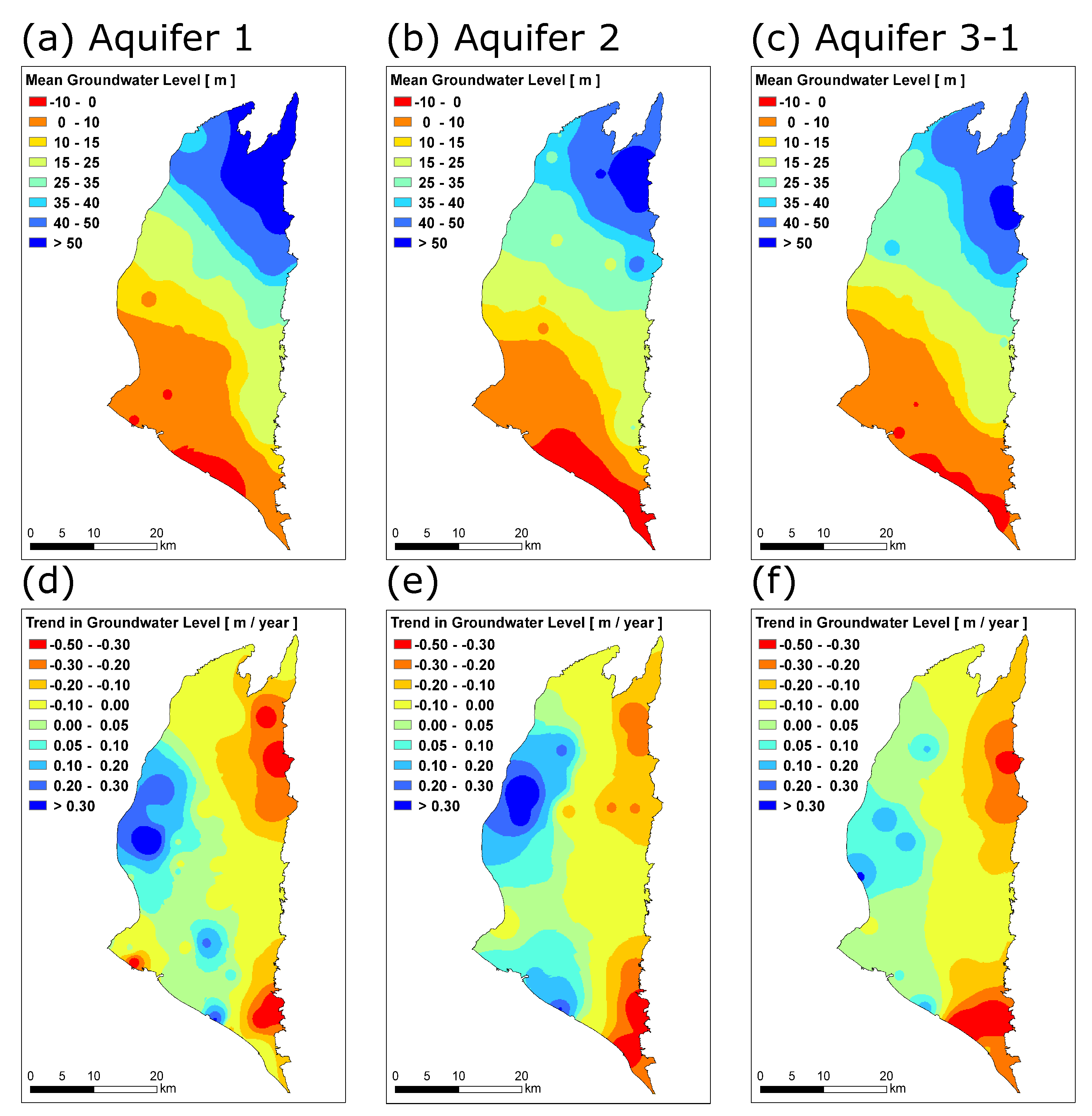
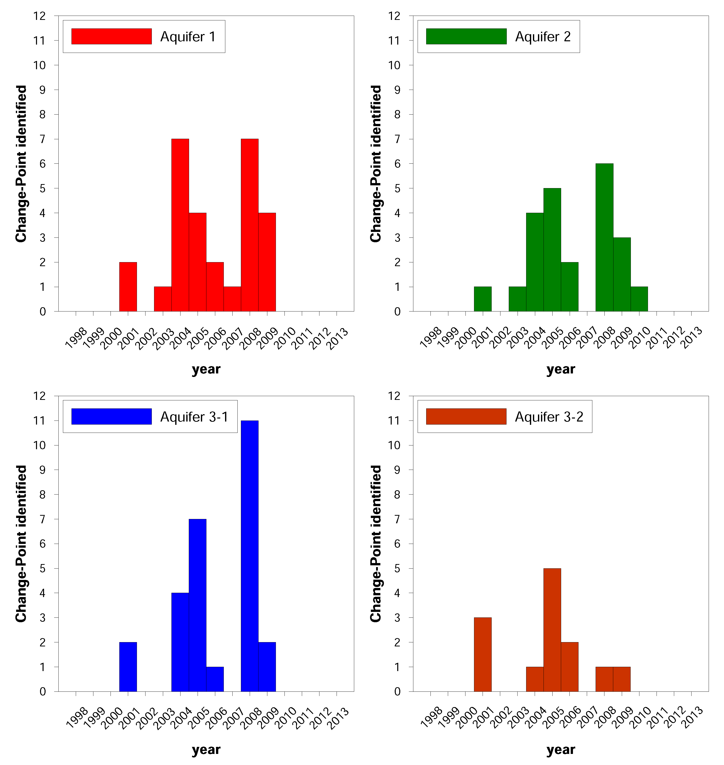
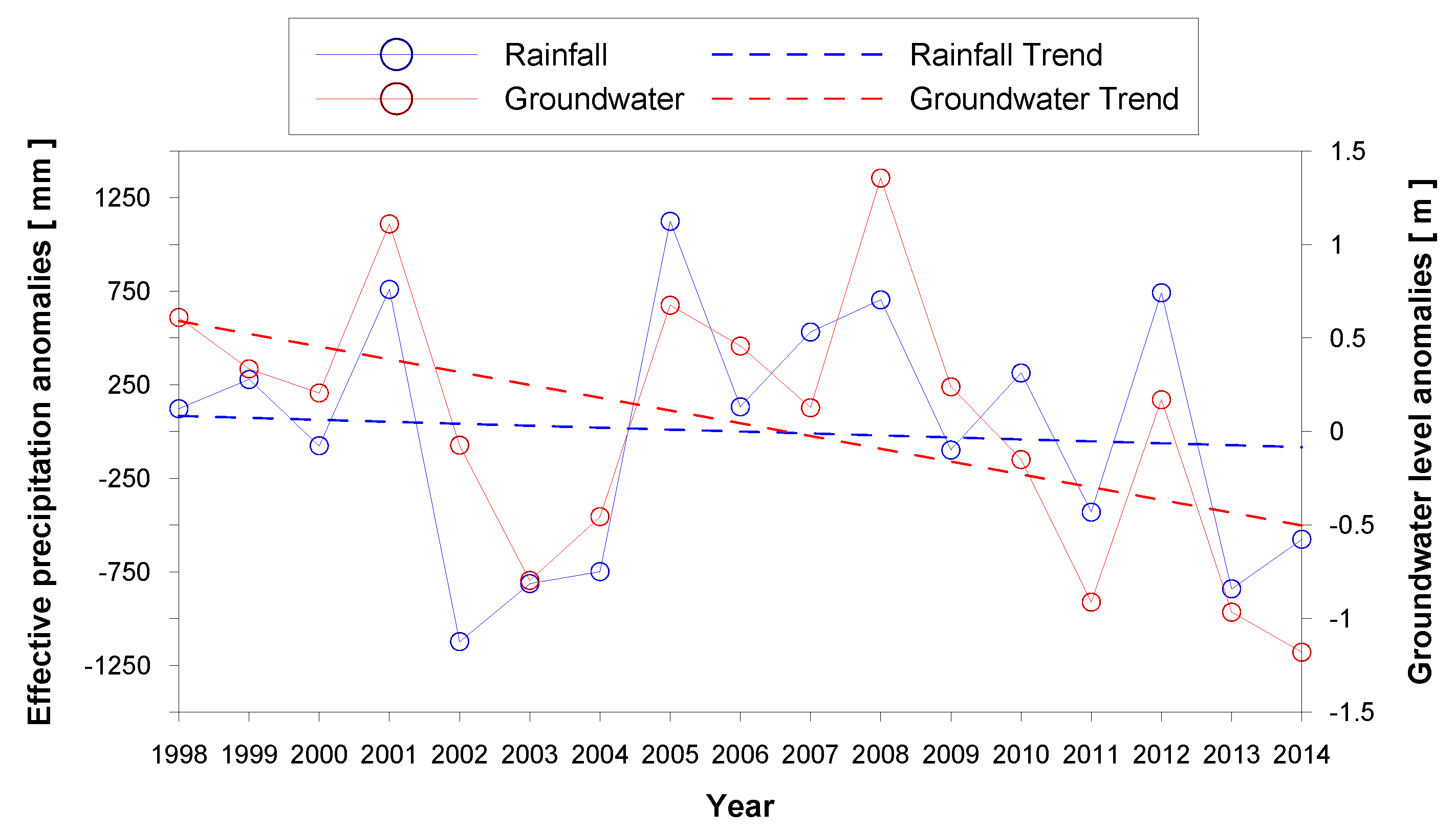
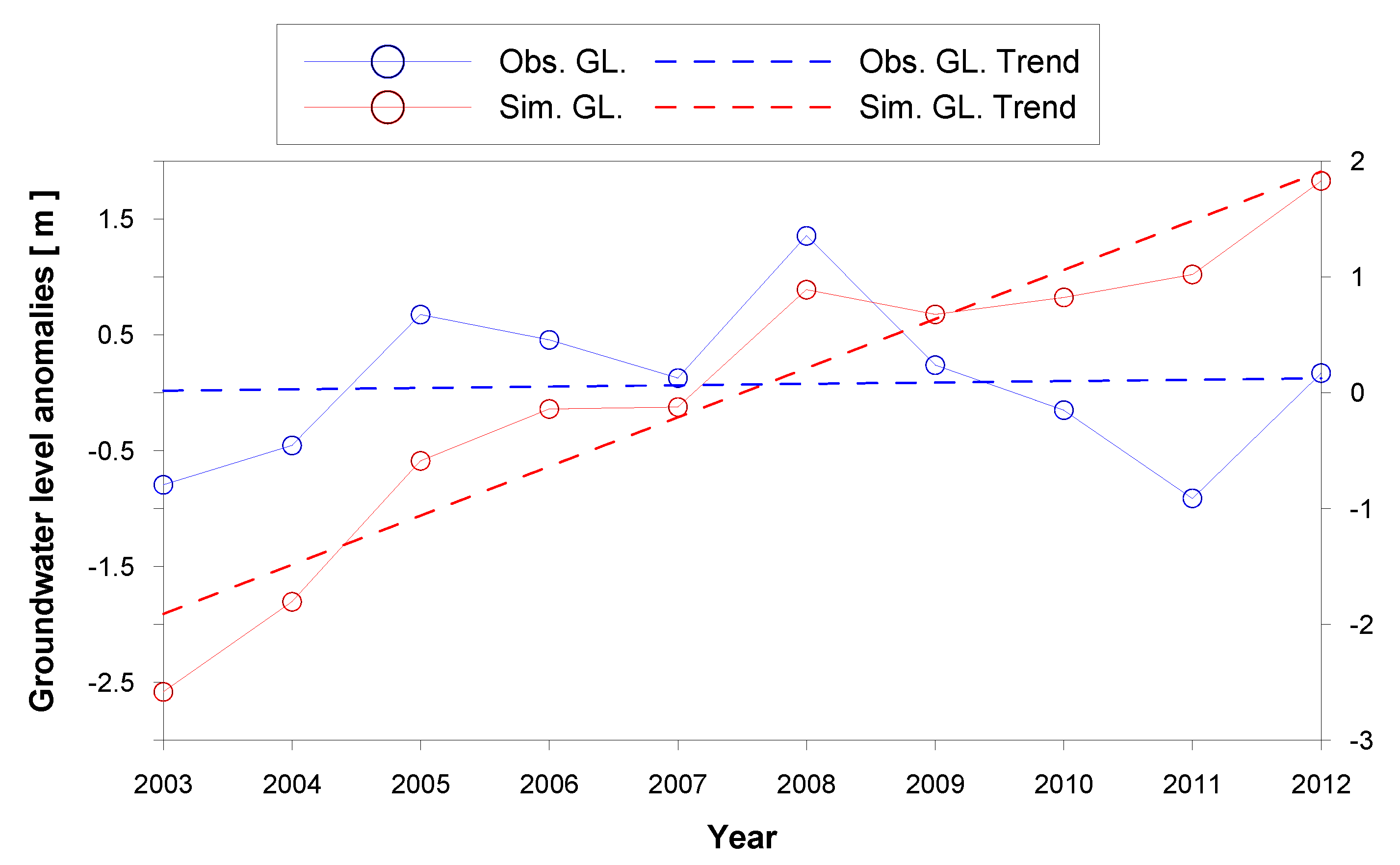
• At the annual scale, quasi-stationary rainfall is not able to provide enough recharge to the PAP aquifers with the observed decline of GLs, especially over the eastern-southeastern part. The decline, aggravated after the identified change points around 2005–2008, suggests a clear association with land subsidence.
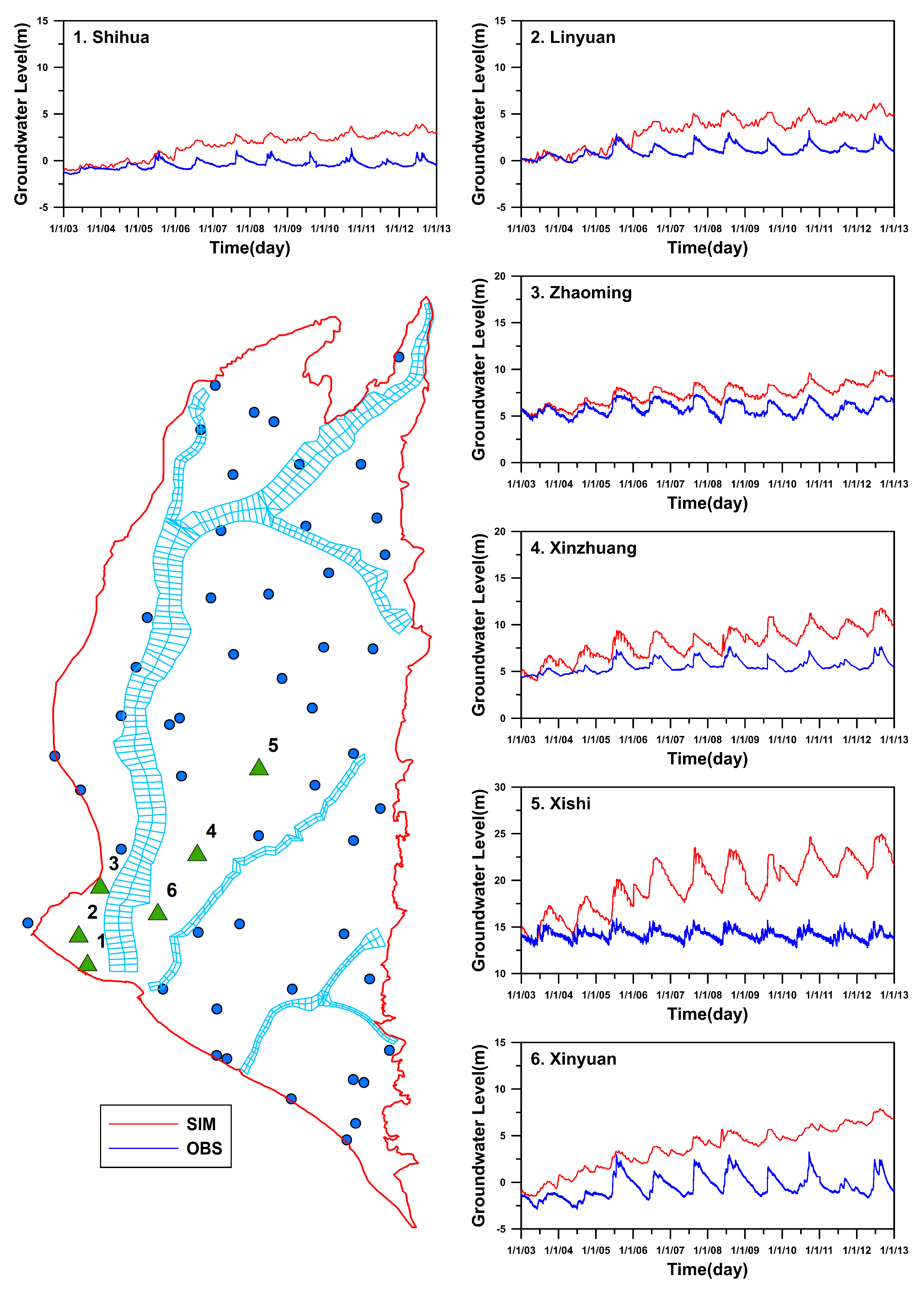
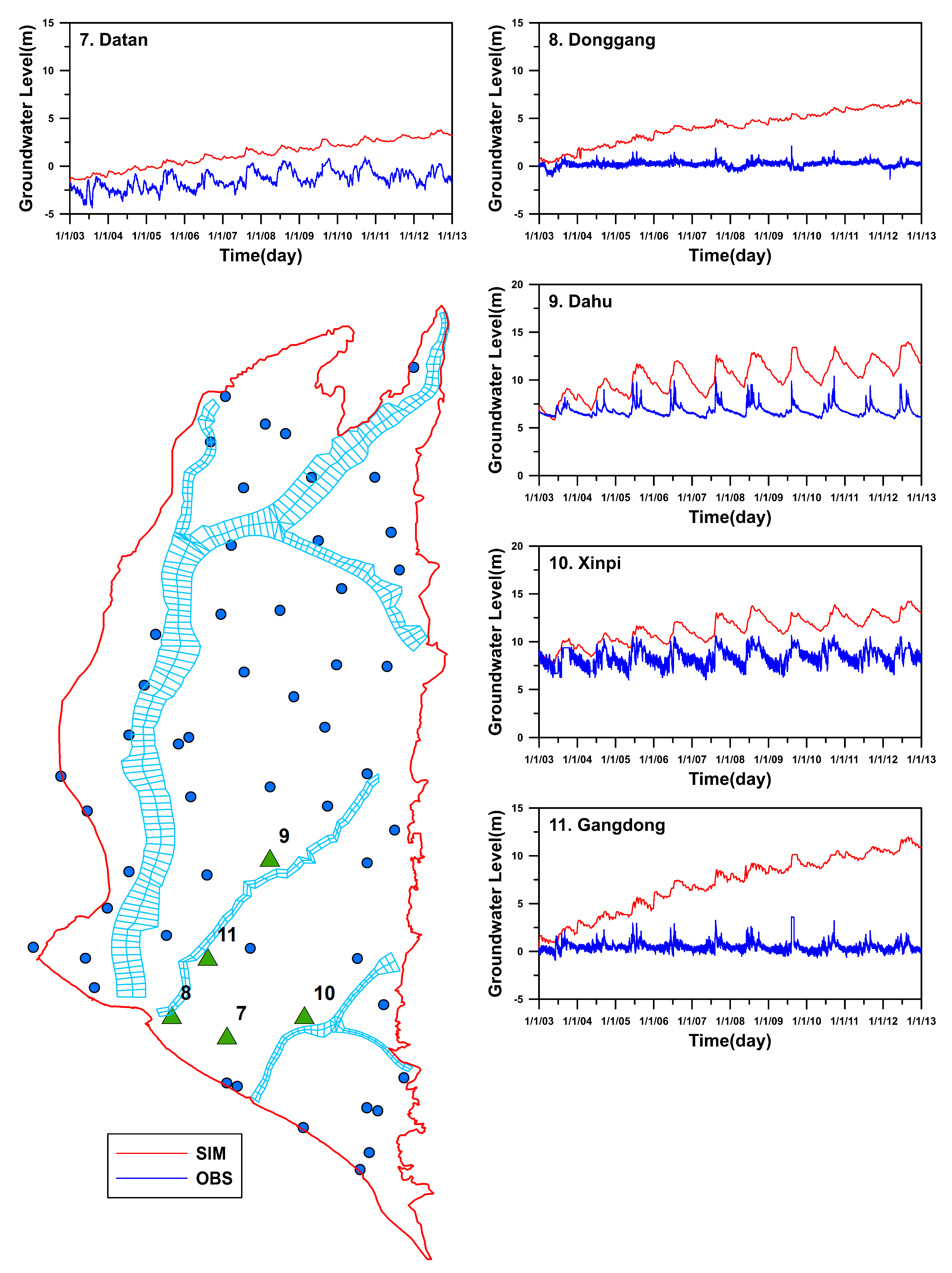
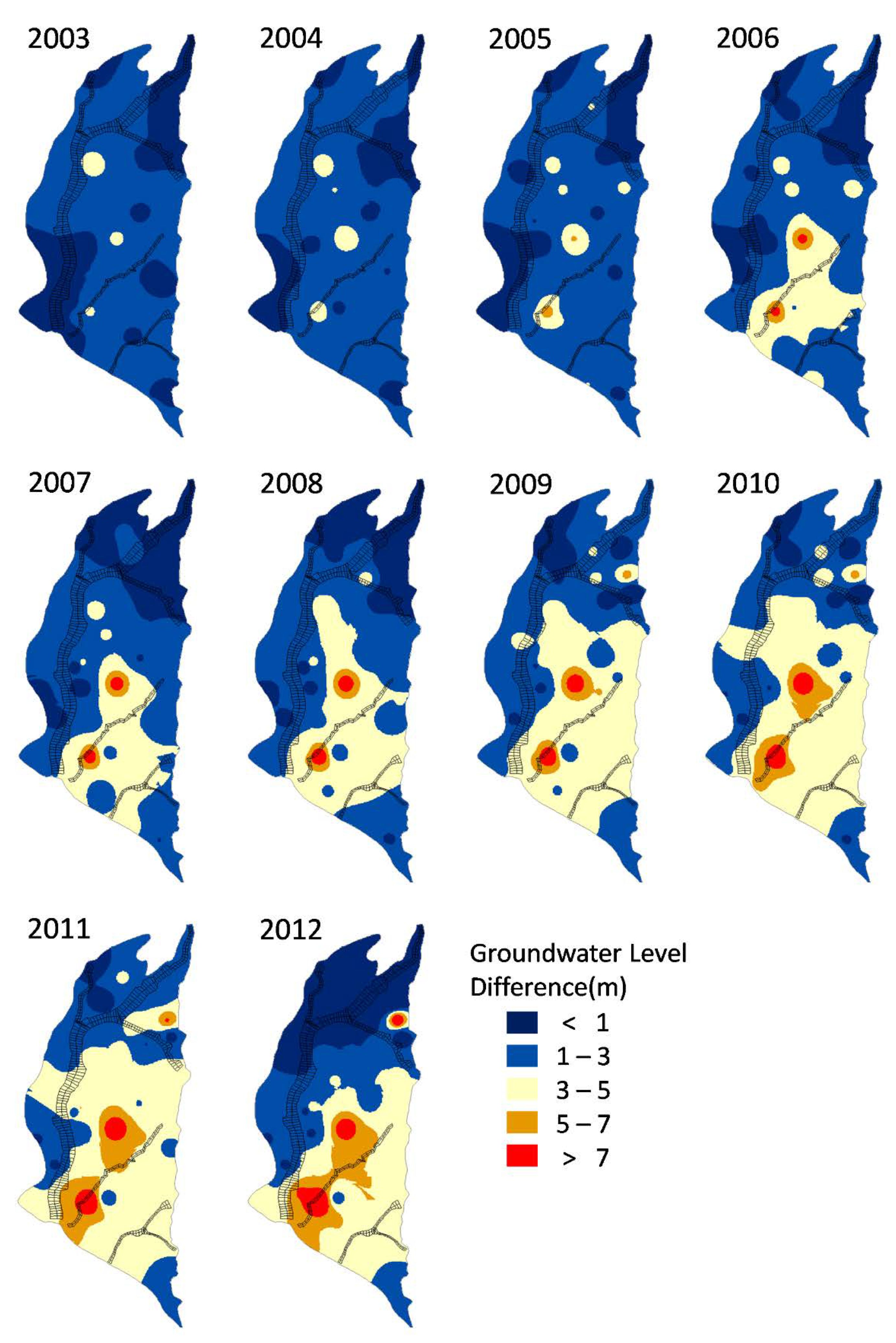
• The pumping-free numerical experiment reveals significant discrepancies between simulated and observed GLs, and these discrepancies develop in both space and time. Our findings not only corroborate the evidence of unregulated/illegal pumping, but also propose a remote connection between pumping and land subsidence.

This case study has been shown as a valuable asset to the WRA, and related regulations are being proposed and legislated to promote a better use of groundwater resource. Several recommendations can be made. For instance, those sites with significant decreases in GLs after the change points should be immediately designated as restricted areas for the restoration of local groundwater resource. The aforementioned agencies are advised to make continual and full use of the developed WASH123D model to inform better management, including the establishment of legal pumping amounts and recharge measures.

References

1. Castle, S.L.; Thomas, B.F.; Reager, J.T.; Rodell, M.; Swenson, S.C.; Famiglietti, J.S. Groundwater depletion during drought threatens future water security of the Colorado River Basin. Geophys. Res. Lett. 2014, 41, 5904–5911. [Google Scholar] [CrossRef] [PubMed] [Green Version]
2. Calow, R.C.; Robins, N.S.; Macdonald, A.M.; Macdonald, D.M.J.; Gibbs, B.R.; Orpen, W.R.G.; Mtembezeka, P.; Andrews, A.J.; Appiah, S.O. Groundwater management in drought-prone areas of Africa. Int. J. Water Resour. Dev. 1997, 13, 241–261. [Google Scholar] [CrossRef]
3. Chai, J.C.; Shen, S.L.; Zhu, H.H.; Zhang, X.L. Land subsidence due to groundwater drawdown in Shanghai. Géotechnique 2004, 54, 143–148. [Google Scholar] [CrossRef]
4. Phien-wej, N.; Giao, P.H.; Nutalaya, P. Land subsidence in Bangkok, Thailand. Eng. Geol. 2006, 82, 187–201. [Google Scholar] [CrossRef]
5. Nishikawa, T.; Siade, A.J.; Reichard, E.G.; Ponti, D.J.; Canales, A.G.; Johnson, T.A. Stratigraphic controls on seawater intrusion and implications for groundwater management, Dominguez Gap area of Los Angeles, California, USA. Hydrogeol. J. 2009, 17, 1699–1725. [Google Scholar] [CrossRef]
6. Petrone, K.C.; Hughes, J.D.; Biel, T.G.V.; Silberstein, R.P. Streamflow decline in southwestern Australia, 1950–2008. Geophys. Res. Lett. 2010, 37, L11401. [Google Scholar] [CrossRef]
7. Hughes, J.D.; Petrone, K.C.; Silberstein, R.P. Drought, groundwater storage and streamflow decline in southwestern Australia. Geophys. Res. Lett. 2012, 39, L03408. [Google Scholar] [CrossRef]
8. Khan, H.F.; Yang, Y.E.; Ringler, C.; Wi, S.; Cheema, M.J.M.; Basharat, M. Guiding groundwater policy in the Indus Basin of Pakistan using a physically based groundwater model. J. Water Resour. Plan. Manag. 2017, 143, 05016014. [Google Scholar] [CrossRef]
9. Domenico, P.A.; Schwartz, F.W. Physical and Chemical Hydrogeology; Wiley: New York, NY, USA, 1998; p. 506. [Google Scholar]
10. Das, B.M. Principles of Geotechnical Engineering; Thomson-Engineering: New York, NY, USA, 2001. [Google Scholar]
11. Kiely, G.; Albertson, J.D.; Parlange, M.B. Recent trends in diurnal variation of precipitation at Valentia on the west coast of Ireland. J. Hydrol. 1998, 207, 270–279. [Google Scholar] [CrossRef] [Green Version]
12. Yu, P.S.; Yang, T.C.; Kuo, C.C. Evaluating long-term trends in annual and seasonal precipitation in Taiwan. Water Resour. Manag. 2006, 20, 1007–1023. [Google Scholar] [CrossRef]
13. Gocic, M.; Trajkovic, S. Analysis of changes in meteorological variables using Mann-Kendall and Sen’s slope estimator statistical tests in Serbia. Glob. Planet. Chang. 2013, 100, 172–182. [Google Scholar] [CrossRef]
14. Gocic, M.; Trajkovic, S. Analysis of precipitation and drought data in Serbia over the period 1980–2010. J. Hydrol. 2013, 494, 32–42. [Google Scholar] [CrossRef]
15. Mahinthakumar, G.; Sayeed, M. Hybrid genetic algorithm–local search methods for solving groundwater source identification inverse problems. J. Water Resour. Plan. Manag. 2005, 131, 45–57. [Google Scholar] [CrossRef]
16. Ayvaz, M.T.; Karahan, H. A simulation/optimization model for the identification of unknown groundwater well locations and pumping rates. J. Hydrol. 2008, 357, 76–92. [Google Scholar] [CrossRef]
17. Sun, P.L.; Yang, C.C.; Lin, T.W. How to amend land subsidence treatment policies to solve coastal subsidence problems in Taiwan. Reg. Environ. Chang. 2011, 11, 679–691. [Google Scholar] [CrossRef]
18. Mann, H.B. Nonparametric tests against trend. Econometrica 1945, 13, 245–259. [Google Scholar] [CrossRef]
19. Kendall, M.G. Rank Correlation Methods; Hafner Pub. Co.: New York, NY, USA, 1962; p. 199. [Google Scholar]
20. Sen, P.K. Estimates of the regression coefficient based on Kendall’s tau. J. Am. Stat. Assoc. 1968, 63, 1379–1389. [Google Scholar] [CrossRef]
21. Pettitt, A.N. A Non-parametric Approach to the Change-point Problem. J. R. Stat. Soc. Ser. C Appl. Stat. 1979, 28, 126–135. [Google Scholar] [CrossRef]
22. Kruskal, W.H.; Wallis, W.A. Use of ranks in one-criterion variance analysis. J. Am. Stat. Assoc. 1952, 47, 583–621. [Google Scholar] [CrossRef]
23. Yeh, G.T.; Cheng, H.P.; Cheng, J.R.; Lin, H.C.; Martin, W.D. A Numerical Model Simulating Water Flow and Contaminant and Sediment Transport in WAterSHed Systems of 1-D Stream-River Network, 2-D Overland Regime, and 3-D Subsurface Media (WASH123D: Version 1.0); U.S. Army Corps of Engineers: Vicksburg, MS, USA, 1998.
24. Yeh, G.T.; Huang, G.B.; Cheng, H.P.; Zhang, F.; Lin, H.C.; Edris, E.; Richards, D. A First-Principle, Physics-Based Watershed Model: WASH123D; CRC Press: Boca Raton, FL, USA, 2005; Chapter 9; pp. 211–244. [Google Scholar]
25. Yates, D.; Purkey, D.; Sieber, J.; Huber-Lee, A.; Galbraith, H.; West, J.; Herrod-Julius, S.; Young, C.; Joyce, B.; Rayej, M. Climate driven water resources model of the Sacramento Basin, California. J. Water Resour. Plan. Manag. 2009, 135, 303–313. [Google Scholar] [CrossRef]
26. Yeh, G.T.; Shih, D.S.; Cheng, J.R.C. An integrated media, integrated processes watershed model. Comput. Fluids 2011, 45, 2–13. [Google Scholar] [CrossRef]
27. Shih, D.S.; Yeh, G.T. Identified model parameterization, calibration, and validation of the physically distributed hydrological model WASH123D in Taiwan. J. Hydrol. Eng. 2010, 16, 126–136. [Google Scholar] [CrossRef]
28. Shih, D.S.; Liau, J.M.; Yeh, G.T. Model assessments of precipitation with a unified regional circulation rainfall and hydrological watershed model. J. Hydrol. Eng. 2011, 17, 43–54. [Google Scholar] [CrossRef]
29. Hsu, T.W.; Shih, D.S.; Li, C.Y.; Lan, Y.J.; Lin, Y.C. A study on coastal flooding and risk assessment under climate change in the mid-western coast of Taiwan. Water 2017, 9, 390. [Google Scholar] [CrossRef]
30. Wu, R.S.; Shih, D.S. Modeling hydrological impacts of groundwater level in the context of climate and land cover change. Terr. Atmos. Ocean. Sci. 2018, 29, 341–353. [Google Scholar] [CrossRef]
31. Ting, C.S.; Zhou, Y.; de Vries, J.J.; Simmers, I. Development of a preliminary ground water flow model for water resources management in the Pingtung Plain. Groundwater 1998, 36, 20–36. [Google Scholar] [CrossRef]
32. Yang, C.C. The Observation and Investigation of Cross Sections in the Valley of Donggang River and Gaoping River; Water Resources Agency: Taipei, Taiwan, 2015. (In Chinese)
33. Li, M.H.; Jang, C.S.; Chen, C.J.; Shih, D.S. Applying Integrated Numerical Modeling of Surface Water and Subsurface Water to Study Groundwater Resources Management (3/3); Water Resources Agency: Taipei, Taiwan, 2016. (In Chinese)
34. Lin, K.P.; Chou, P.C.; Shih, D.S. To study hydrological variabilities by using surface and groundwater coupled model–A case study of Pingtung plain, Taiwan. Procedia Eng. 2016, 154, 1034–1042. [Google Scholar] [CrossRef]
35. Hamon, R.W. Computation of direct runoff amounts from storm rainfall. Int. Assoc. Hydrol. Sci. 1963, 63, 52–62. [Google Scholar]
Figure 1. Map of the Pingtung Alluvial Plain (PAP) in Southwest Taiwan.
Water 11 00360 g001
Figure 2. Spatial locations of various stations, including groundwater level, streamflow, rainfall, and weather stations.
Water 11 00360 g002
Figure 3. The (top) panel illustrates the hydrogeological units (please refer to Table 1 for the definition of each unit), and the (bottom) shows the 3D mesh over the PAP used for WASH123D simulations.
Water 11 00360 g003
Figure 4. The (top) and (bottom) panel shows the spatial distribution of annual rainfall amounts (mean rainfall intensity) and the corresponding trend over the PAP.
Water 11 00360 g004
Figure 5. The (top) panel shows the spatial distribution of mean groundwater levels in Aquifers 1, 2, and 3-1, and the (bottom) shows the estimated trends in the corresponding aquifers over the PAP.
Water 11 00360 g005
Figure 6. Histograms of identified change points for each aquifer, representing frequency distributions of identified years when groundwater level series at any gauges experience a shift in the mean.
Water 11 00360 g006
Figure 7. The (top) and (bottom) panel shows the estimated trends in groundwater levels prior (posterior) to the identified change points at each gauge.
Water 11 00360 g007
Figure 8. Annual series of average effective precipitation and groundwater level anomalies in Aquifer 3-1 and corresponding linear trends.
Water 11 00360 g008
Figure 9. Validation results of river stages in the Gaoping River (left) and groundwater levels (right) from 8 June–8 July of 2012 when Tropical Storm Talim affected Taiwan.
Water 11 00360 g009
Figure 10. Comparisons between simulated and observed groundwater level series at selected sites along the downstream of the Gaoping River from 2003–2013.
Water 11 00360 g010
Figure 11. As in Figure 10, but for the downstream of the Donggang and Linbian Rivers.
Water 11 00360 g011
Figure 12. Evolution of the spatial patterns of groundwater level differences (simulated minus observed data) for the 10-year simulation.
Water 11 00360 g012
Figure 13. Annual series of observed and simulated groundwater level anomalies and corresponding linear trends. GL, groundwater level.
Water 11 00360 g013